Enhanced Ninth-Order Memory-Based Iterative Technique for Efficiently Solving Nonlinear Equations

Abstract

In this article, we present a novel three-step with-memory iterative method for solving nonlinear equations. We have improved the convergence order of a well-known optimal eighth-order iterative method by converting it into a with-memory version. The Hermite interpolating polynomial is utilized to compute a self-accelerating parameter that improves the convergence order. The proposed uni-parametric with-memory iterative method improves its R-order of convergence from 8 to $8.8989$. Additionally, no more function evaluations are required to achieve this improvement in convergence order. Furthermore, the efficiency index has increased from $1.6818$ to $1.7272$. The proposed method is shown to be more effective than some well-known existing methods, as shown by extensive numerical testing on a variety of problems.

1. Introduction

Many complex problems in science and engineering involve nonlinear equations of the form $\zeta \left(x\right)=0$, where $\zeta :D\subset \mathbb{R}\to \mathbb{R}$ is a scalar function defined over an open interval D. Solutions to these equations typically cannot be expressed in closed form. As traditional analytical methods are often insufficient for solving such equations, iterative numerical techniques have become indispensable, especially with advancements in computational technology that enable more efficient and accurate solutions. Newton’s method [1] is a widely used iterative technique for approximating the simple root $\xi$ of $\zeta \left(x\right)=0$. It follows the iterative formula:

$$x_{n+1}=x_n-{\displaystyle \frac{\zeta \left(x_n\right)}{\zeta \prime \left(x_n\right)}},n=0,1,2,\cdots$$

(1)

where $\zeta$ is the function and $\zeta \prime$ is its derivative. Newton’s method is known for its quadratic convergence near the root and it requires the evaluation of both the function and its derivative in each iteration. Researchers continue to refine Newton’s method to improve convergence rates and enhance its practical applicability. Multipoint iterative methods have emerged as the most efficient root-solvers, surpassing the theoretical limitations of one-point methods in terms of convergence order and computational efficiency. These advantages have led to a surge in interest in multipoint methods in the current era. The advancement of symbolic computation and multi-precision arithmetic has further accelerated their development.

However, while improving the convergence rate is advantageous, it may also lead to a higher number of function evaluations, which can ultimately decrease the efficiency index of these methods. The efficiency index, as discussed in [2], measures the balance between the order of convergence and the number of functional evaluations per step, represented by the formula $E={\rho }^{1/\gamma }$, where $\rho$ is the order of convergence and $\gamma$ is the number of functional and derivative evaluations conducted per iteration. Researchers have a particular interest in developing accelerated multipoint methods with memory due to their high computational efficiency. They aim to enhance the order of these methods beyond the limits of optimal methods, guided by Kung–Traub’s conjecture, which posits that $n+1$ function evaluations can achieve the optimal convergence order of $2^n$ [2].

However, iterative methods that incorporate memory leverage the state of recent and previous iterations to increase the efficiency index as well as the convergence order. Significant efforts have been made recently in the field to expand without-memory methods to with-memory methods by employing self-accelerating parameters. Liu et al. [3] upgraded a single-step without-memory method with a second order of convergence to a with-memory method using one self-accelerating parameter and achieved a fourth order of convergence. Sharma et al. [4] upgraded an eighth-order without-memory iterative method to a with-memory method using two self-accelerating parameters and attained a tenth order of convergence. Additionally, Thangkhenpau et al. [5] developed a derivative-free without-memory iterative method with an eighth order of convergence and then expanded it to a with-memory method using four self-accelerating parameters, which resulted in an increase in the convergence order from 8 to 15.5156. In recent years, the development of with-memory iterative methods has garnered considerable interest among researchers. Notable contributors to the development of with-memory methods include Choubey et al. [6,7,8], Raziyeh Erfanifar [9], Howk et al. [10], Sharma et al. [11,12], Wang and Zhang [13], Liu et al. [14], and Panday et al. [15].

In this article, we proposed a new three-step, uni-parametric, with-memory iterative technique while involving complex error computations. It is designed for modular implementation to facilitate practical adoption in solving nonlinear equations efficiently and it improves the R-order of convergence from 8 to 8.8989. An efficiency index of 1.7272 is attained by this method. By adding a self-accelerating parameter to the third step of an existing optimal eighth-order without-memory iterative technique [16] and conducting a comprehensive convergence analysis, a new uni-parametric three-point with-memory iterative method was developed, as described in Section 2. A detailed assessment using numerical tests is presented in Section 3, which offers a thorough comparison of the suggested method with other well-established methods. Section 4 provides a comprehensive summary of the research findings and their implications.

2. Analysis of Convergence for With-Memory Method

In this section, we use a parameter $\alpha$ in the third step of the three-step optimal eighth-order scheme proposed by Matthies et al. [16] in 2016, to increase its order of convergence from eight to nine. After adding the parameter $\alpha$ in the third step of [16], we obtain

$$\begin{array}{cc}\hfill y_n& =x_n-{\displaystyle \frac{\zeta \left(x_n\right)}{\zeta \prime \left(x_n\right)}},\hfill \\ \hfill z_n& =x_n-{\displaystyle \frac{\zeta \left(x_n\right)}{\zeta \prime \left(x_n\right)}}\left(1+{\displaystyle \frac{\zeta \left(y_n\right)}{\zeta \left(x_n\right)}}+\left(1+{\displaystyle \frac{1}{1+\frac{\zeta \left(x_n\right)}{\zeta \prime \left(x_n\right)}}}\right){\left({\displaystyle \frac{\zeta \left(y_n\right)}{\zeta \left(x_n\right)}}\right)}^2\right),\hfill \\ \hfill x_{n+1}& =z_n-{\displaystyle \frac{\zeta \left(z_n\right)}{\zeta [z_n,y_n]+(z_n-y_n)\zeta [z_n,y_n,x_n]+(z_n-y_n)(z_n-x_n)\zeta [z_n,y_n,x_n,x_n]+\alpha \zeta \left(z_n\right)}},\hfill \end{array}$$

(2)

where $\zeta [z_n,y_n]$, $\zeta [z_n,y_n,x_n]$, and $\zeta [z_n,y_n,x_n,x_n]$ represent the divided differences and are defined by $\zeta [z_n,y_n]={\displaystyle \frac{\zeta \left(z_n\right)-\zeta \left(y_n\right)}{z_n-y_n}}$, $\zeta [z_n,y_n,x_n]={\displaystyle \frac{\zeta [z_n,y_n]-\zeta [y_n,x_n]}{z_n-x_n}}$, and $\zeta [z_n,y_n,x_n,x_n]={\displaystyle \frac{\zeta [z_n,y_n,x_n]-\zeta [y_n,x_n,x_n]}{z_n-x_n}}$.

Using Taylor-series approximation, the expressions for $\zeta \left(x_n\right)$ and $\zeta \prime \left(x_n\right)$ can be written as

$$\begin{array}{c}\hfill \zeta \left(x_n\right)=A(e_n+c_2{e}_n^2+c_3{e}_n^3+c_4{e}_n^4+c_5{e}_n^5+c_6{e}_n^6+c_7{e}_n^7+c_8{e}_n^8)+O\left(e_n^9\right),\end{array}$$

(3)

$$\begin{array}{c}\hfill \zeta \prime \left(x_n\right)=A(1+2c_2{e}_n+3c_3{e}_n^2+4c_4{e}_n^3+5c_5{e}_n^4+6c_6{e}_n^5+7c_7{e}_n^6+8c_8{e}_n^7+9c_9{e}_n^8)+O\left(e_n^9\right),\end{array}$$

(4)

where $A=\zeta \prime \left(\xi \right)$, $\xi$ is the simple root of $\zeta \left(x\right)$, $e_n=x_n-\xi$, and $c_j$ = ${\displaystyle \frac{{\zeta }^{\left(j\right)}\left(\xi \right)}{j!\zeta \prime \left(\xi \right)}}$ for $j=2,3,\cdots$.

Now, the error expressions for the first two sub-steps of (2) is given by [16]:

$$\begin{array}{c}\hfill e_{n,y}=c_2{e}_n^2+\left(-2c_2^2+2c_3\right)e_n^3+\left(4c_2^3-7c_2{c}_3+3c_4\right)e_n^4+O\left(e_n^5\right),\end{array}$$

(5)

$$\begin{array}{cc}\hfill e_{n,z}=& c_2\left(c_2+5c_2^2-c_3\right)e_n^4\hfill \\ \hfill & +\left(-8c_2^3-36c_2^4-2c_3^2+c_2^2(-1+32c_3)+c_2(4c_3-2c_4)\right)e_n^5+O\left(e_n^6\right),\hfill \end{array}$$

(6)

and we obtain the error expansion for the third sub-step of (2) as:

$$\begin{array}{cc}\hfill e_{n+1}=& c_2^2\left(c_2+5c_2^2-c_3\right)\left((\alpha +c_2)(c_2+5c_2^2-c_3)+c_4\right)e_n^8\hfill \\ \hfill & -c_2(8(19+45\alpha )c_2^6+360c_2^7+2c_2^5(13+76\alpha -196c_3)+4c_3^2(-\alpha c_3+c_4)\hfill \\ \hfill & +c_2^4\left(2+26\alpha -8(15+49\alpha )c_3+66c_4\right)+2c_2^3(\alpha -5(1+12\alpha )c_3+42c_3^2\hfill \\ \hfill & +(7+10\alpha )c_4-5c_5)+c_2^2\left(2c_3(-5\alpha +6(1+7\alpha )c_3)+c_4+4(\alpha -12c_3)c_4-2c_5\right)\hfill \\ \hfill & +2c_2\left(6\alpha c_3^2-2c_3^3+c_4^2+c_3(-\left((3+2\alpha )c_4\right)+c_5)\right))e_n^9+O\left(e_n^{10}\right),\hfill \end{array}$$

(7)

where $e_{n,y}$ = $y_n-\xi$, $e_{n,z}$ = $z_n-\xi$, and $\alpha \in R$. We obtain the following with-memory iterative scheme by replacing $\alpha$ with a self-accelerating parameter ${\alpha }_n$ in (2):

$$\begin{array}{cc}\hfill y_n& =x_n-{\displaystyle \frac{\zeta \left(x_n\right)}{\zeta \prime \left(x_n\right)}},\hfill \\ \hfill z_n& =x_n-{\displaystyle \frac{\zeta \left(x_n\right)}{\zeta \prime \left(x_n\right)}}\left(1+{\displaystyle \frac{\zeta \left(y_n\right)}{\zeta \left(x_n\right)}}+\left(1+{\displaystyle \frac{1}{1+\frac{\zeta \left(x_n\right)}{\zeta \prime \left(x_n\right)}}}\right){\left({\displaystyle \frac{\zeta \left(y_n\right)}{\zeta \left(x_n\right)}}\right)}^2\right),\hfill \\ \hfill x_{n+1}& =z_n-{\displaystyle \frac{\zeta \left(z_n\right)}{\zeta [z_n,y_n]+(z_n-y_n)\zeta [z_n,y_n,x_n]+(z_n-y_n)(z_n-x_n)\zeta [z_n,y_n,x_n,x_n]+{\alpha }_n\zeta \left(z_n\right)}}.\hfill \end{array}$$

(8)

The above scheme is represented by NWM9. Now, from (7), it is clear that the convergence order of the algorithm (2) is eight when $\alpha \ne -{\displaystyle \frac{c_4}{c_2+5c_2^2-c_3}}-c_2$. Next, to accelerate the order of convergence of the algorithm presented in (8) from eight to nine, we can assume $\alpha =-{\displaystyle \frac{c_4}{c_2+5c_2^2-c_3}}-c_2=-{\displaystyle \frac{{\zeta }^{\left(iv\right)}\left(\xi \right)\zeta \prime \left(\xi \right)}{12\zeta ″\left(\xi \right)\zeta \prime \left(\xi \right)+30{(\zeta ″\left(\xi \right))}^2-4\zeta ‴\left(\xi \right)\zeta \prime \left(\xi \right)}}-{\displaystyle \frac{\zeta ″\left(\xi \right)}{2\zeta \prime \left(\xi \right)}}$, but in reality, the exact values of $\zeta \prime \left(\xi \right),\zeta ″\left(\xi \right),\zeta ‴\left(\xi \right)$, and ${\zeta }^{\left(iv\right)}\left(\xi \right)$ are not attainable in practice. So, we assume the parameter $\alpha$ as ${\alpha }_n$. The parameter ${\alpha }_n$ can be calculated by using the available data from the current and previous iterations and satisfies the condition ${lim}_{n\to \infty }{\alpha }_n=-{\displaystyle \frac{c_4}{c_2+5c_2^2-c_3}}-c_2=-{\displaystyle \frac{{\zeta }^{\left(iv\right)}\left(\xi \right)\zeta \prime \left(\xi \right)}{12\zeta ″\left(\xi \right)\zeta \prime \left(\xi \right)+30{(\zeta ″\left(\xi \right))}^2-4\zeta ‴\left(\xi \right)\zeta \prime \left(\xi \right)}}-{\displaystyle \frac{\zeta ″\left(\xi \right)}{2\zeta \prime \left(\xi \right)}}$ such that the eighth-order asymptotic convergence constant should be zero in the error expression (7). The formula for ${\alpha }_n$ is as follows:

$${\alpha }_n=-{\displaystyle \frac{H_7^{\left(iv\right)}\left(z_n\right)\zeta \prime \left(x_n\right)}{12H_5^{″}\left(x_n\right)\zeta \prime \left(x_n\right)+30{\left(H_5^{″}\left(x_n\right)\right)}^2-4H_6^{‴}\left(y_n\right)\zeta \prime \left(x_n\right)}}-{\displaystyle \frac{H_5^{″}\left(x_n\right)}{2\zeta \prime \left(x_n\right)}},$$

(9)

where the Hermite interpolating polynomials $H_m\left(x\right)$ for $m=5,6,7$ are given by

$$\begin{array}{cc}\hfill H_7\left(x\right)=& \zeta \left(z_n\right)+(x-z_n)\zeta [z_n,y_n]+(x-z_n)(x-y_n)\zeta [z_n,y_n,x_n]\hfill \\ \hfill & +(x-z_n)(x-y_n)(x-x_n)\zeta [z_n,y_n,x_n,x_n]+(x-z_n)(x-y_n){(x-x_n)}^2\hfill \\ \hfill & \zeta [z_n,y_n,x_n,x_n,z_{n-1}]+(x-z_n)(x-y_n){(x-x_n)}^2(x-z_{n-1})\hfill \\ \hfill & \zeta [z_n,y_n,x_n,x_n,z_{n-1},y_{n-1}]+(x-z_n)(x-y_n){(x-x_n)}^2(x-z_{n-1})(x-y_{n-1})\hfill \\ \hfill & \zeta [z_n,y_n,x_n,x_n,z_{n-1},y_{n-1},x_{n-1}]+(x-z_n)(x-y_n){(x-x_n)}^2(x-z_{n-1})\hfill \\ \hfill & (x-y_{n-1})(x-x_{n-1})\zeta [z_n,y_n,x_n,x_n,z_{n-1},y_{n-1},x_{n-1},x_{n-1}],\hfill \end{array}$$

$$\begin{array}{cc}\hfill H_6\left(x\right)=& \zeta \left(y_n\right)+(x-y_n)\zeta [y_n,x_n]+(x-y_n)(x-x_n)\zeta [y_n,x_n,x_n]\hfill \\ \hfill & +(x-y_n){(x-x_n)}^2\zeta [y_n,x_n,x_n,z_{n-1}]+(x-y_n){(x-x_n)}^2(x-z_{n-1})\hfill \\ \hfill & \zeta [y_n,x_n,x_n,z_{n-1},y_{n-1}]+(x-y_n){(x-x_n)}^2(x-z_{n-1})(x-y_{n-1})\hfill \\ & \zeta [y_n,x_n,x_n,z_{n-1},y_{n-1},x_{n-1}]+(x-y_n){(x-x_n)}^2(x-z_{n-1})(x-y_{n-1})\hfill \\ \hfill & (x-x_{n-1})\zeta [y_n,x_n,x_n,z_{n-1},y_{n-1},x_{n-1},x_{n-1}],\hfill \end{array}$$

$$\begin{array}{cc}\hfill H_5\left(x\right)=& \zeta \left(x_n\right)+(x-x_n)\zeta [x_n,x_n]+{(x-x_n)}^2\zeta [x_n,x_n,z_{n-1}]\hfill \\ \hfill & +{(x-x_n)}^2(x-z_{n-1})\zeta [x_n,x_n,z_{n-1},y_{n-1}]+{(x-x_n)}^2(x-z_{n-1})(x-y_{n-1})\hfill \\ \hfill & \zeta [x_n,x_n,z_{n-1},y_{n-1},x_{n-1}]+{(x-x_n)}^2(x-z_{n-1})(x-y_{n-1})(x-x_{n-1})\hfill \\ & \zeta [x_n,x_n,z_{n-1},y_{n-1},x_{n-1},x_{n-1}],\hfill \end{array}$$

Note: The condition $H_m^{\prime }\left(x_n\right)=\zeta \prime \left(x_n\right)$ is satisfied by the Hermite interpolation polynomial $H_m\left(x\right)$ for $m=5,6,7.$ So, ${\alpha }_n=-{\displaystyle \frac{H_7^{\left(iv\right)}\left(z_n\right)\zeta \prime \left(x_n\right)}{12H_5^{″}\left(x_n\right)\zeta \prime \left(x_n\right)+30{\left(H_5^{″}\left(x_n\right)\right)}^2-4H_6^{‴}\left(y_n\right)\zeta \prime \left(x_n\right)}}-{\displaystyle \frac{H_5^{″}\left(x_n\right)}{2\zeta \prime \left(x_n\right)}}$ can be expressed as ${\alpha }_n=-{\displaystyle \frac{H_7^{\left(iv\right)}\left(z_n\right)H_m^{\prime }\left(x_n\right)}{12H_5^{″}\left(x_n\right)H_m^{\prime }\left(x_n\right)+30{\left(H_5^{″}\left(x_n\right)\right)}^2-4H_6^{‴}\left(y_n\right)H_m^{\prime }\left(x_n\right)}}-{\displaystyle \frac{H_5^{″}\left(x_n\right)}{2H_m^{\prime }\left(x_n\right)}}$ for $m=5,6,7.$

Theorem 1.

Let $H_m$ be the Hermite polynomial of degree m, interpolating the function ζ at interpolation nodes $z_n,y_n,x_n,x_n,z_{n-1},y_{n-1},x_{n-1},x_{n-1}$ within an interval $D\subset \mathbb{R}$ and the derivative ${\zeta }^{(m+1)}$ is continuous in D with $H_m\left(x_n\right)=\zeta \left(x_n\right)$ and $H_m^{\prime }\left(x_n\right)=\zeta \prime \left(x_n\right)$. Suppose that all nodes $z_n,y_n,x_n,x_n,z_{n-1},y_{n-1},x_{n-1},x_{n-1}$ are in the neighborhood of the root ξ. Then,

$$H_7^{\left(iv\right)}\left(z_n\right)=24\zeta \prime \left(\xi \right)(c_4-c_8{e}_{n-1,z}{e}_{n-1,y}{e}_{n-1}^2),$$

(10)

$$H_6^{‴}\left(y_n\right)=6\zeta \prime \left(\xi \right)(c_3-c_7{e}_{n-1,z}{e}_{n-1,y}{e}_{n-1}^2),$$

(11)

$$H_5^{″}\left(x_n\right)=2\zeta \prime \left(\xi \right)(c_2-c_6{e}_{n-1,z}{e}_{n-1,y}{e}_{n-1}^2),$$

(12)

and

$$\begin{array}{cc}\hfill {\alpha }_n=& -{\displaystyle \frac{H_7^{\left(iv\right)}\left(z_n\right)\zeta \prime \left(x_n\right)}{12H_5^{″}\left(x_n\right)\zeta \prime \left(x_n\right)+30{\left(H_5^{″}\left(x_n\right)\right)}^2-4H_6^{‴}\left(y_n\right)\zeta \prime \left(x_n\right)}}-{\displaystyle \frac{H_5^{″}\left(x_n\right)}{2\zeta \prime \left(x_n\right)}}\hfill \\ \hfill & \sim -{\displaystyle \frac{c_4}{c_2+5c_2^2-c_3}}-c_2+{\displaystyle \frac{c_2}{c_2+5c_2^2-c_3}}{e}_{n-1,z}{e}_{n-1,y}{e}_{n-1}^2-{\displaystyle \frac{c_6{c}_8}{c_2+5c_2^2-c_3}}{e}_{n-1,z}^2{e}_{n-1,y}^2{e}_{n-1}^4\hfill \\ \hfill & +{\displaystyle \frac{5c_2^2{c}_8}{c_2+5c_2^2-c_3}}{e}_{n-1,z}{e}_{n-1,y}{e}_{n-1}^2+{\displaystyle \frac{5c_6^2{c}_8}{c_2+5c_2^2-c_3}}{e}_{n-1,z}^3{e}_{n-1,y}^3{e}_{n-1}^6\hfill \\ \hfill & -{\displaystyle \frac{10c_2{c}_6{c}_8}{c_2+5c_2^2-c_3}}{e}_{n-1,z}{e}_{n-1,y}{e}_{n-1}^2-{\displaystyle \frac{c_3{c}_8}{c_2+5c_2^2-c_3}}{e}_{n-1,z}{e}_{n-1,y}{e}_{n-1}^2\hfill \\ \hfill & +{\displaystyle \frac{c_7{c}_8}{c_2+5c_2^2-c_3}}{e}_{n-1,z}^2{e}_{n-1,y}^2{e}_{n-1}^4.\hfill \end{array}$$

(13)

Again, after simplification, we have

$$\begin{array}{cc}\hfill {\alpha }_n+{\displaystyle \frac{c_4}{c_2+5c_2^2-c_3}}+c_2& =({\alpha }_n+c_2)(c_2+5c_2^2-c_3)+c_4\hfill \\ \hfill & \sim ({\displaystyle \frac{c_2}{c_2+5c_2^2-c_3}}-{\displaystyle \frac{c_6{c}_8}{c_2+5c_2^2-c_3}}{e}_{n-1,z}{e}_{n-1,y}{e}_{n-1}^2+{\displaystyle \frac{5c_2^2{c}_8}{c_2+5c_2^2-c_3}}\hfill \\ \hfill & +{\displaystyle \frac{5c_6^2{c}_8}{c_2+5c_2^2-c_3}}{e}_{n-1,z}^2{e}_{n-1,y}^2{e}_{n-1}^4-{\displaystyle \frac{10c_2{c}_6{c}_8}{c_2+5c_2^2-c_3}}-{\displaystyle \frac{c_3{c}_8}{c_2+5c_2^2-c_3}}\hfill \\ \hfill & +{\displaystyle \frac{c_7{c}_8}{c_2+5c_2^2-c_3}}{e}_{n-1,z}{e}_{n-1,y}{e}_{n-1}^2)e_{n-1,z}{e}_{n-1,y}{e}_{n-1}^2.\hfill \end{array}$$

(14)

Proof. 

We can calculate the expression of the seventh-degree, sixth-degree, and fifth-degree Hermite interpolation polynomial as

$$\zeta \left(x\right)-H_7\left(x\right)={\displaystyle \frac{{\zeta }^{\left(8\right)}\left(\delta \right)}{8!}}(x-z_n)(x-y_n){(x-x_n)}^2(x-z_{n-1})(x-y_{n-1}){(x-x_{n-1})}^2,$$

(15)

$$\zeta \left(x\right)-H_6\left(x\right)={\displaystyle \frac{{\zeta }^{\left(7\right)}\left(\delta \right)}{7!}}(x-y_n){(x-x_n)}^2(x-z_{n-1})(x-y_{n-1}){(x-x_{n-1})}^2,$$

(16)

$$\zeta \left(x\right)-H_5\left(x\right)={\displaystyle \frac{{\zeta }^{\left(6\right)}\left(\delta \right)}{6!}}{(x-x_n)}^2(x-z_{n-1})(x-y_{n-1}){(x-x_{n-1})}^2.$$

(17)

Now, we obtain the below-mentioned equations by rearranging and differentiating Equation (15) four times at the point $x=z_n$, Equation (16) three times at the point $x=y_n$, and Equation (17) two times at the point $x=x_n$, respectively.

$$H_7^{\left(iv\right)}\left(z_n\right)={\zeta }^{\left(iv\right)}\left(z_n\right)-24{\displaystyle \frac{{\zeta }^{\left(8\right)}\left(\delta \right)}{8!}}(z_n-z_{n-1})(z_n-y_{n-1}){(z_n-x_{n-1})}^2,$$

(18)

$$H_6^{‴}\left(y_n\right)=\zeta ‴\left(y_n\right)-6{\displaystyle \frac{{\zeta }^{\left(7\right)}\left(\delta \right)}{7!}}(y_n-z_{n-1})(y_n-y_{n-1}){(y_n-x_{n-1})}^2,$$

(19)

$$H_5^{″}\left(x_n\right)=\zeta ″\left(x_n\right)-2{\displaystyle \frac{{\zeta }^{\left(6\right)}\left(\delta \right)}{6!}}(x_n-z_{n-1})(x_n-y_{n-1}){(x_n-x_{n-1})}^2.$$

(20)

Next, Taylor’s series expansion of $\zeta \prime$ at the points $z_n$, $y_n$, and $x_n$ in D and $\delta \in D$ about the zero $\xi$ of $\zeta$ provides

$$\zeta \prime \left(x_n\right)=\zeta \prime \left(\xi \right)\left(1+2c_2{e}_n+3c_3{e}_n^2+O\left(e_n^3\right)\right),$$

(21)

$$\zeta ″\left(x_n\right)=\zeta \prime \left(\xi \right)\left(2c_2+6c_3{e}_n+O\left(e_n^2\right)\right),$$

(22)

$$\zeta ‴\left(y_n\right)=\zeta \prime \left(\xi \right)\left(6c_3+24c_4{e}_{n,y}+O\left(e_{n,y}^2\right)\right).$$

(23)

Similarly,

$${\zeta }^{\left(iv\right)}\left(z_n\right)=\zeta \prime \left(\xi \right)\left(24c_4+120c_5{e}_{n,z}+O\left(e_{n,z}^2\right)\right),$$

(24)

$${\zeta }^{\left(6\right)}\left(\delta \right)=\zeta \prime \left(\xi \right)\left(6!c_6+7!c_7{e}_{\delta }+O\left(e_{\delta }^2\right)\right),$$

(25)

$${\zeta }^{\left(7\right)}\left(\delta \right)=\zeta \prime \left(\xi \right)\left(7!c_7+8!c_8{e}_{\delta }+O\left(e_{\delta }^2\right)\right),$$

(26)

$${\zeta }^{\left(8\right)}\left(\delta \right)=\zeta \prime \left(\xi \right)\left(8!c_8+9!c_9{e}_{\delta }+O\left(e_{\delta }^2\right)\right),$$

(27)

where $e_{\delta }=\delta -\xi$. Putting (24) and (27) in (18), (23) and (26) in (19), and (22) and (25) in (20), we obtain

$$H_7^{\left(iv\right)}\left(z_n\right)=24\zeta \prime \left(\xi \right)(c_4-c_8{e}_{n-1,z}{e}_{n-1,y}{e}_{n-1}^2),$$

(28)

$$H_6^{‴}\left(y_n\right)=6\zeta \prime \left(\xi \right)(c_3-c_7{e}_{n-1,z}{e}_{n-1,y}{e}_{n-1}^2),$$

(29)

and

$$H_5^{″}\left(x_n\right)=2\zeta \prime \left(\xi \right)(c_2-c_6{e}_{n-1,z}{e}_{n-1,y}{e}_{n-1}^2),$$

(30)

Using Equations (21), (28), (29) and (30), we have

$$\begin{array}{cc}\hfill & -{\displaystyle \frac{H_7^{\left(iv\right)}\left(z_n\right)\zeta \prime \left(x_n\right)}{12H_5^{″}\left(x_n\right)\zeta \prime \left(x_n\right)+30{\left(H_5^{″}\left(x_n\right)\right)}^2-4H_6^{‴}\left(y_n\right)\zeta \prime \left(x_n\right)}}-{\displaystyle \frac{H_5^{″}\left(x_n\right)}{2\zeta \prime \left(x_n\right)}}\hfill \\ \hfill & \sim -{\displaystyle \frac{c_4}{c_2+5c_2^2-c_3}}-c_2+{\displaystyle \frac{c_2}{c_2+5c_2^2-c_3}}{e}_{n-1,z}{e}_{n-1,y}{e}_{n-1}^2-{\displaystyle \frac{c_6{c}_8}{c_2+5c_2^2-c_3}}{e}_{n-1,z}^2{e}_{n-1,y}^2{e}_{n-1}^4\hfill \\ \hfill & +{\displaystyle \frac{5c_2^2{c}_8}{c_2+5c_2^2-c_3}}{e}_{n-1,z}{e}_{n-1,y}{e}_{n-1}^2+{\displaystyle \frac{5c_6^2{c}_8}{c_2+5c_2^2-c_3}}{e}_{n-1,z}^3{e}_{n-1,y}^3{e}_{n-1}^6\hfill \\ \hfill & -{\displaystyle \frac{10c_2{c}_6{c}_8}{c_2+5c_2^2-c_3}}{e}_{n-1,z}{e}_{n-1,y}{e}_{n-1}^2-{\displaystyle \frac{c_3{c}_8}{c_2+5c_2^2-c_3}}{e}_{n-1,z}{e}_{n-1,y}{e}_{n-1}^2\hfill \\ \hfill & +{\displaystyle \frac{c_7{c}_8}{c_2+5c_2^2-c_3}}{e}_{n-1,z}^2{e}_{n-1,y}^2{e}_{n-1}^4.\hfill \end{array}$$

(31)

And hence,

$$\begin{array}{cc}\hfill {\alpha }_n\sim & -{\displaystyle \frac{c_4}{c_2+5c_2^2-c_3}}-c_2+({\displaystyle \frac{c_2}{c_2+5c_2^2-c_3}}-{\displaystyle \frac{c_6{c}_8}{c_2+5c_2^2-c_3}}{e}_{n-1,z}{e}_{n-1,y}{e}_{n-1}^2\hfill \\ \hfill & +{\displaystyle \frac{5c_2^2{c}_8}{c_2+5c_2^2-c_3}}+{\displaystyle \frac{5c_6^2{c}_8}{c_2+5c_2^2-c_3}}{e}_{n-1,z}^2{e}_{n-1,y}^2{e}_{n-1}^4-{\displaystyle \frac{10c_2{c}_6{c}_8}{c_2+5c_2^2-c_3}}-{\displaystyle \frac{c_3{c}_8}{c_2+5c_2^2-c_3}}\hfill \\ \hfill & +{\displaystyle \frac{c_7{c}_8}{c_2+5c_2^2-c_3}}{e}_{n-1,z}{e}_{n-1,y}{e}_{n-1}^2)e_{n-1,z}{e}_{n-1,y}{e}_{n-1}^2.\hfill \end{array}$$

(32)

or

$$\begin{array}{cc}\hfill {\alpha }_n+{\displaystyle \frac{c_4}{c_2+5c_2^2-c_3}}+c_2& =({\alpha }_n+c_2)(c_2+5c_2^2-c_3)+c_4\hfill \\ \hfill & \sim ({\displaystyle \frac{c_2}{c_2+5c_2^2-c_3}}-{\displaystyle \frac{c_6{c}_8}{c_2+5c_2^2-c_3}}{e}_{n-1,z}{e}_{n-1,y}{e}_{n-1}^2+{\displaystyle \frac{5c_2^2{c}_8}{c_2+5c_2^2-c_3}}\hfill \\ \hfill & +{\displaystyle \frac{5c_6^2{c}_8}{c_2+5c_2^2-c_3}}{e}_{n-1,z}^2{e}_{n-1,y}^2{e}_{n-1}^4-{\displaystyle \frac{10c_2{c}_6{c}_8}{c_2+5c_2^2-c_3}}-{\displaystyle \frac{c_3{c}_8}{c_2+5c_2^2-c_3}}\hfill \\ \hfill & +{\displaystyle \frac{c_7{c}_8}{c_2+5c_2^2-c_3}}{e}_{n-1,z}{e}_{n-1,y}{e}_{n-1}^2)e_{n-1,z}{e}_{n-1,y}{e}_{n-1}^2.\hfill \end{array}$$

(33)

This completes the proof of Theorem 1. □

The definition of R-order of convergence [17] and the statement in [18] can be used to estimate the order of convergence of the iterative scheme (8).

Theorem 2.

If the errors $e_j=x_j-\xi$ evaluated by an iterative root-finding method IM fulfill

$$e_{k+1}\sim \prod _{i=0}^{m-2}{\left(e_{k-i}\right)}^{m_i},k\ge k\left(\left\{e_k\right\}\right)$$

(34)

then the R-order of convergence of IM, denoted with $O_R(IM,\xi )$, satisfies the inequality $O_R(IM,\xi )\ge s^{*}$, where $s^{*}$ is the unique positive solution of the equation $s_{n+1}-{\sum }_{i=0}^n{m}_i{s}^{n-i}=0$ [18].

Proof. 

The proof of the above Theorem 2 can be found in [18]. □

Presently, for the new iterative scheme with memory (8), we can state the subsequent convergence theorem.

Theorem 3.

In the iterative method (8), let ${\alpha }_n$ be a varying parameter, calculated by Equation (9). If an initial guess $x_0$ is sufficiently near to a simple zero ξ of $\zeta \left(x\right)$, then the R-order of convergence of the iterative method (8) with memory is at least 8.8989.

Proof. 

Let the iterative method (IM) generate the sequence of $\left\{x_n\right\}$ which converges to the root $\xi$ of $\zeta \left(x\right)$. By means of R-order $O_R(IM,\xi )\ge r$, we express

$$\begin{array}{cc}\hfill e_{n+1}\sim & D_{n,r}{e}_n^r,\hfill \end{array}$$

(35)

and

$$\begin{array}{cc}\hfill e_n\sim & D_{n-1,r}{e}_{n-1}^r.\hfill \end{array}$$

(36)

Next, $D_{n,r}$ will tend to the asymptotic error constant $D_r$ of $IM$ by taking $n\to \infty$; then,

$$e_{n+1}\sim D_{n,r}{\left(D_{n-1,r}{e}_{n-1}^r\right)}^r=D_{n,r}{D}_{n-1,r}^r{e}_{n-1}^{r^2}.$$

(37)

The resulting error expression of the with-memory scheme (8) can be obtained using (5)–(7) and the varying parameter ${\alpha }_n$.

$$\begin{array}{c}\hfill e_{n,y}=y_n-\xi \sim c_2{e}_n^2,\end{array}$$

(38)

$$\begin{array}{c}\hfill e_{n,z}=z_n-\xi \sim c_2(c_2+5c_2^2-c_3)e_n^4,\end{array}$$

(39)

and

$$\begin{array}{c}\hfill e_{n+1}=x_{n+1}-\xi \sim c_2^2\left(c_2+5c_2^2-c_3\right)\left((\alpha +c_2)(c_2+5c_2^2-c_3)+c_4\right)e_n^8.\end{array}$$

(40)

Here, the higher-order terms in Equations (38)–(40) are excluded.

Now, let the R-order convergence of the iterative sequences $\left\{y_n\right\}$ and $\left\{z_n\right\}$ be p and q, respectively; then,

$$e_{n,y}\sim D_{n,p}{e}_n^p\sim D_{n,p}{\left(D_{n-1,r}{e}_{n-1}^r\right)}^p=D_{n,p}{D}_{n-1,r}^p{e}_{n-1}^{rp},$$

(41)

and

$$e_{n,z}\sim D_{n,q}{e}_n^q\sim D_{n,q}{\left(D_{n-1,r}{e}_{n-1}^r\right)}^q=D_{n,q}{D}_{n-1,r}^q{e}_{n-1}^{rq}.$$

(42)

Now, by Equations (36) and (38), we obtain

$$\begin{array}{c}\hfill e_{n,y}\sim c_2{e}_n^2\sim c_2{\left(D_{n-1,r}{e}_{n-1}^r\right)}^2\sim c_2{D}_{n-1,r}^2{e}_{n-1}^{2r}.\end{array}$$

(43)

Also, by Equations (36) and (39), we obtain

$$\begin{array}{cc}\hfill e_{n,z}& \sim c_2(c_2+5c_2^2-c_3)e_n^4\hfill \\ \hfill & \sim c_2(c_2+5c_2^2-c_3){\left(D_{n-1,r}{e}_{n-1}^r\right)}^4\hfill \\ \hfill & \sim c_2(c_2+5c_2^2-c_3)D_{n-1,r}^4{e}_{n-1}^{4r}.\hfill \end{array}$$

(44)

Again, by Equations (33), (36) and (40), we have

$$\begin{array}{cc}\hfill e_{n+1}& \sim c_2^2\left(c_2+5c_2^2-c_3\right)\left((\alpha +c_2)(c_2+5c_2^2-c_3)+c_4\right)e_n^8\hfill \\ \hfill & \sim c_2^2\left(c_2+5c_2^2-c_3\right)({\displaystyle \frac{c_2}{c_2+5c_2^2-c_3}}-{\displaystyle \frac{c_6{c}_8}{c_2+5c_2^2-c_3}}{e}_{n-1,z}{e}_{n-1,y}{e}_{n-1}^2+{\displaystyle \frac{5c_2^2{c}_8}{c_2+5c_2^2-c_3}}\hfill \\ \hfill & +{\displaystyle \frac{5c_6^2{c}_8}{c_2+5c_2^2-c_3}}{e}_{n-1,z}^2{e}_{n-1,y}^2{e}_{n-1}^4-{\displaystyle \frac{10c_2{c}_6{c}_8}{c_2+5c_2^2-c_3}}-{\displaystyle \frac{c_3{c}_8}{c_2+5c_2^2-c_3}}\hfill \\ \hfill & +{\displaystyle \frac{c_7{c}_8}{c_2+5c_2^2-c_3}}{e}_{n-1,z}{e}_{n-1,y}{e}_{n-1}^2)e_{n-1,z}{e}_{n-1,y}{e}_{n-1}^2{\left(D_{n-1,r}{e}_{n-1}^r\right)}^8\hfill \\ \hfill & \sim c_2^2\left(c_2+5c_2^2-c_3\right)({\displaystyle \frac{c_2}{c_2+5c_2^2-c_3}}-{\displaystyle \frac{c_6{c}_8}{c_2+5c_2^2-c_3}}{e}_{n-1,z}{e}_{n-1,y}{e}_{n-1}^2+{\displaystyle \frac{5c_2^2{c}_8}{c_2+5c_2^2-c_3}}\hfill \\ \hfill & +{\displaystyle \frac{5c_6^2{c}_8}{c_2+5c_2^2-c_3}}{e}_{n-1,z}^2{e}_{n-1,y}^2{e}_{n-1}^4-{\displaystyle \frac{10c_2{c}_6{c}_8}{c_2+5c_2^2-c_3}}-{\displaystyle \frac{c_3{c}_8}{c_2+5c_2^2-c_3}}\hfill \\ \hfill & +{\displaystyle \frac{c_7{c}_8}{c_2+5c_2^2-c_3}}{e}_{n-1,z}{e}_{n-1,y}{e}_{n-1}^2)D_{n-1,q}{e}_{n-1}^q{D}_{n-1,p}{e}_{n-1}^p{e}_{n-1}^2{\left(D_{n-1,r}{e}_{n-1}^r\right)}^8\hfill \\ \hfill & \sim c_2^2\left(c_2+5c_2^2-c_3\right)({\displaystyle \frac{c_2}{c_2+5c_2^2-c_3}}-{\displaystyle \frac{c_6{c}_8}{c_2+5c_2^2-c_3}}{e}_{n-1,z}{e}_{n-1,y}{e}_{n-1}^2+{\displaystyle \frac{5c_2^2{c}_8}{c_2+5c_2^2-c_3}}\hfill \\ \hfill & +{\displaystyle \frac{5c_6^2{c}_8}{c_2+5c_2^2-c_3}}{e}_{n-1,z}^2{e}_{n-1,y}^2{e}_{n-1}^4-{\displaystyle \frac{10c_2{c}_6{c}_8}{c_2+5c_2^2-c_3}}-{\displaystyle \frac{c_3{c}_8}{c_2+5c_2^2-c_3}}\hfill \\ \hfill & +{\displaystyle \frac{c_7{c}_8}{c_2+5c_2^2-c_3}}{e}_{n-1,z}{e}_{n-1,y}{e}_{n-1}^2)D_{n-1,q}{D}_{n-1,p}{D}_{n-1,r}^8{e}_{n-1}^{8r+p+q+2}.\hfill \end{array}$$

(45)

since $r>q>p$. By equating the exponents of $e_{n-1}$ present in the set of relations (41)–(43), (42)–(44), and (37)–(45), we attain the resulting system of equations:

$$\begin{array}{cc}\hfill rp& =2r\hfill \\ \hfill rq& =4r\hfill \\ \hfill r^2& =8r+p+q+2\hfill \end{array}$$

(46)

The solution of the system of Equation (46) is specified by $r=8.8989$, $q=4$, and $p=2$. As a result, the R-order of convergence of the with-memory iterative method (8) is at least $8.8989$. □

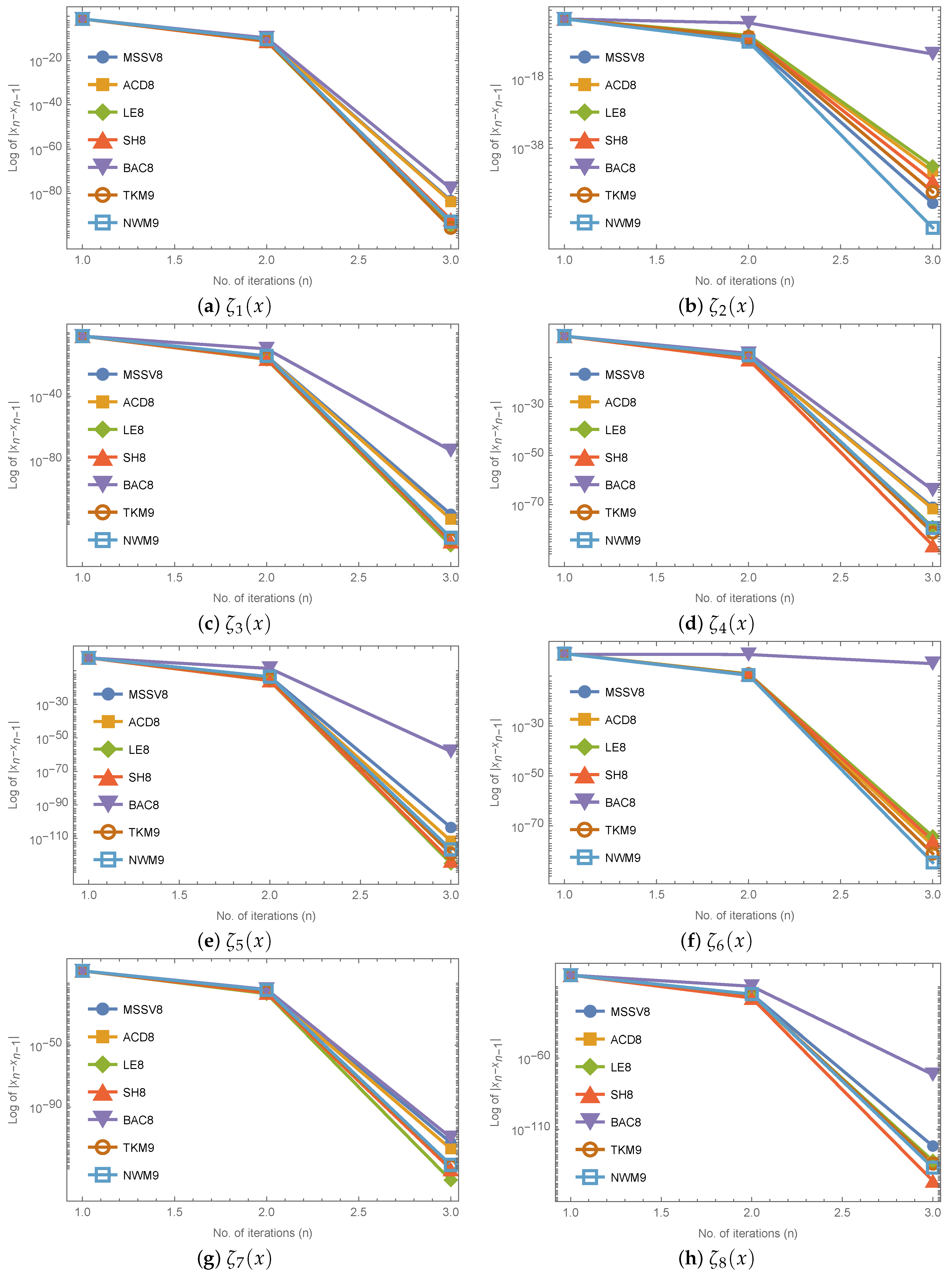
3. Numerical Discussion

This section examines the convergence behavior of the newly developed with-memory technique NWM9 introduced in (8). Our goal is to evaluate the effectiveness of a recently developed iterative method by applying it to a variety of nonlinear problems. The nonlinear test functions, along with their roots and initial guesses for our numerical analysis, are described below:

• Example 1: ${\zeta }_1\left(x\right)=1+x^2·e^{cosx/2}-(x+1)e^{sinx/2}$, $x_0=0.9$, $\xi \approx 0.8475$
• Example 2: ${\zeta }_2\left(x\right)=e^{x^3+cosx+1}-x^2+x+1$, $x_0=-0.8$, $\xi \approx -1.0787$
• Example 3: ${\zeta }_3\left(x\right)=x·e^{x^2}-{sin}^{2}x+3cosx+5$, $x_0=-1.2$, $\xi \approx -1.2076$
• Example 4: ${\zeta }_4\left(x\right)=e^{-x^2}(1+x^3+x^6)(x-2)$, $x_0=1.95$, $\xi \approx 2.0000$
• Example 5: ${\zeta }_5\left(x\right)=x^7-4x^4+x-1$, $x_0=1.58$, $\xi \approx 1.5749$
• Example 6: ${\zeta }_6\left(x\right)=e^{x^2-4}+sin(x-2)-x^4+15$, $x_0=2.1$, $\xi \approx 2.0000$
• Example 7: ${\zeta }_7\left(x\right)=e^{-x^2+x+2}-1$, $x_0=2.01$, $\xi \approx 2.0000$
• Example 8 [19,20]: In civil engineering, beams in mathematical models are horizontal elements that support loads and span openings, sometimes called lintels if made of stone or brick. “Floor joist” or “roof joist” designates beams supporting floors or roofs, respectively. Stringers support lighter bridge deck loads, while floor beams handle heavier transverse loads. Girders, constructed from metal plates or concrete, bear terminal loads of smaller beams, enhancing rigidity and extending spans. Various nonlinear mathematical models have been developed to specify the precise beam location. The model below is an example which was taken from [19,20]:

  $${\zeta }_8\left(x\right)=x^4+4x^3-24x^2+16x+16=0.$$

  (47)

The roots of the above fourth-order polynomial are 2, 2 and $-4\pm 2\sqrt{3}$ and the initial guess for ${\zeta }_8\left(x\right)$ is taken as $x_0=-0.55$”.

We compare our method NWM9 (8) to various well-established methods published in the literature, including MSSV8 (48), ACD8 (49), LE8 (50), SH8 (51), BAC8 (52), and TKM9 (53), which are discussed below:

In 2016, Matthies et al. (MSSV8) [16] developed an optimal eighth-order iterative method which is defined as

$$\begin{array}{cc}\hfill y_n& =x_n-{\displaystyle \frac{\zeta \left(x_n\right)}{\zeta \prime \left(x_n\right)}},\hfill \\ \hfill z_n& =x_n-{\displaystyle \frac{\zeta \left(x_n\right)}{\zeta \prime \left(x_n\right)}}\left(1+{\displaystyle \frac{\zeta \left(y_n\right)}{\zeta \left(x_n\right)}}+\left(1+{\displaystyle \frac{1}{1+\frac{\zeta \left(x_n\right)}{\zeta \prime \left(x_n\right)}}}\right){\left({\displaystyle \frac{\zeta \left(y_n\right)}{\zeta \left(x_n\right)}}\right)}^2\right),\hfill \\ \hfill x_{n+1}& =z_n-{\displaystyle \frac{\zeta \left(z_n\right)}{\zeta [z_n,y_n]+(z_n-y_n)\zeta [z_n,y_n,x_n]+(z_n-y_n)(z_n-x_n)\zeta [z_n,y_n,x_n,x_n]}}.\hfill \end{array}$$

(48)

In 2024, Abdullah et al. (ACD8) [21] developed an optimal eighth-order iterative method which is defined as

$$\begin{array}{cc}\hfill y_n& =x_n-{\displaystyle \frac{\zeta \left(x_n\right)}{\zeta \prime \left(x_n\right)}},\hfill \\ \hfill z_n& =x_n-{\displaystyle \frac{\zeta \left(x_n\right)(\zeta {\left(x_n\right)}^3+2\zeta \left(x_n\right)\zeta {\left(y_n\right)}^2)}{\zeta \prime \left(x_n\right)(\zeta \left(x_n\right)-\zeta \left(y_n\right))(\zeta {\left(x_n\right)}^2+\zeta {\left(y_n\right)}^2)}},\hfill \\ \hfill x_{n+1}& =z_n-{\displaystyle \frac{\zeta \left(z_n\right)(z_n-y_n)}{\zeta \left(z_n\right)-\zeta \left(y_n\right)}}(A\left(u_n\right)+B\left(v_n\right)+H\left(w_n\right)),\hfill \end{array}$$

(49)

where $u_n={\displaystyle \frac{\zeta \left(z_n\right)}{\zeta \left(y_n\right)}}$, $v_n={\displaystyle \frac{\zeta \left(z_n\right)}{\zeta \left(x_n\right)}}$, and $w_n={\displaystyle \frac{\zeta \left(y_n\right)}{\zeta \left(x_n\right)}}$.

In 2014, Lotfi and Eftekhari (LE8) [22] developed an optimal eighth-order iterative method which is defined as

$$\begin{array}{cc}\hfill y_n& =x_n-{\displaystyle \frac{\zeta \left(x_n\right)}{\zeta \prime \left(x_n\right)}},\hfill \\ \hfill z_n& =y_n-{\displaystyle \frac{\zeta \left(x_n\right)}{\zeta \left(x_n\right)-2\zeta \left(y_n\right)}}{\displaystyle \frac{\zeta \left(y_n\right)}{\zeta \prime \left(x_n\right)}},\hfill \\ \hfill x_{n+1}& =z_n-(K\left(t_1\right)\times L\left(t_2\right)\times P\left(t_3\right)){\displaystyle \frac{\zeta \left(z_n\right)\zeta [x_n,y_n]}{\zeta [x_n,z_n]\zeta [y_n,z_n]}},\hfill \end{array}$$

(50)

where $t_1={\displaystyle \frac{\zeta \left(z_n\right)}{\zeta \left(x_n\right)}}$, $t_2={\displaystyle \frac{\zeta \left(y_n\right)}{\zeta \left(x_n\right)}}$, and $t_3={\displaystyle \frac{\zeta \left(z_n\right)}{\zeta \left(y_n\right)}}$.

In 2020, Solaiman and Hashim (SH8) [23] developed an optimal eighth-order iterative method which is defined as

$$\begin{array}{cc}\hfill y_n& =x_n-{\displaystyle \frac{\zeta \left(x_n\right)}{\zeta \prime \left(x_n\right)}},\hfill \\ \hfill z_n& =y_n-{\displaystyle \frac{\zeta \left(y_n\right)}{\zeta \prime \left(y_n\right)}}-{\displaystyle \frac{2{\left(\zeta \left(y_n\right)\right)}^2\zeta \prime \left(y_n\right)R(x_n,y_n)}{4{(\zeta \prime \left(y_n\right))}^4-4\zeta \left(y_n\right){(\zeta \prime \left(y_n\right))}^{2}R(x_n,y_n)+{(\zeta \prime \left(y_n\right))}^2{\left(R(x_n,y_n)\right)}^2}},\hfill \\ \hfill x_{n+1}& =z_n-{\displaystyle \frac{\zeta \left(z_n\right)}{\zeta \prime \left(z_n\right)}},\hfill \end{array}$$

(51)

where $\zeta \prime \left(y_n\right)$, $\zeta \prime \left(z_n\right)$, and $R(x_n,y_n)$ are approximated as

$\zeta \prime \left(y_n\right)\approx 2\zeta [y_n,x_n]-\zeta \prime \left(x_n\right).$

$\zeta \prime \left(z_n\right)\approx \zeta [z_n,x_n](2+{\displaystyle \frac{x_n-z_n}{y_n-z_n}})-{\displaystyle \frac{{(x_n-z_n)}^2}{(x_n-y_n)(y_n-z_n)}}\zeta [x_n,y_n]+\zeta \prime \left(x_n\right){\displaystyle \frac{y_n-z_n}{x_n-y_n}}.$

$R(x_n,y_n)\approx \left[3{\displaystyle \frac{\zeta \left(y_n\right)-\zeta \left(x_n\right)}{y_n-x_n}}-2\zeta \prime \left(y_n\right)-\zeta \prime \left(x_n\right)\right]{\displaystyle \frac{2}{x_n-y_n}}$.

In 2020, Behl et al. (BAC8) [24] developed an optimal eighth-order iterative method which is defined as

$$\begin{array}{cc}\hfill w_n& =x_n+\beta \zeta \left(x_n\right);\beta \in R,\hfill \\ \hfill y_n& =x_n-{\displaystyle \frac{\zeta \left(x_n\right)}{\zeta [w_n,x_n]}},\hfill \\ \hfill z_n& =y_n-{\displaystyle \frac{\zeta \left(w_n\right)\zeta \left(y_n\right)(y_n-x_n)}{(\zeta \left(w_n\right)-\zeta \left(y_n\right))(\zeta \left(y_n\right)-\zeta \left(x_n\right))}},\hfill \\ \hfill x_{n+1}& =z_n-{\displaystyle \frac{\zeta \left(z_n\right)(w_n-x_n)(w_n-y_n)(x_n-y_n)}{\zeta [y_n,z_n](w_n-x_n)(w_n-z_n)(x_n-z_n)-a(y_n-z_n)}},\hfill \end{array}$$

(52)

where $a=\zeta [x_n,z_n](w_n-y_n)(w_n-z_n)-\zeta [w_n,z_n](x_n-y_n)(x_n-z_n)$.

In 2021, Torkashvand et al. (TKM9) [25] proposed a family of with-memory iterative methods with a ninth order of convergence which is defined as

$$\begin{array}{cc}\hfill w_n& =x_n+{\beta }_n\zeta \left(x_n\right),\hfill \\ \hfill y_n& =x_n-{\displaystyle \frac{\zeta \left(x_n\right)}{\zeta [x_n,w_n]}},\hfill \\ \hfill z_n& =y_n-{\displaystyle \frac{\zeta [x_n,y_n]-\zeta [y_n,w_n]+\zeta [x_n,w_n]}{\zeta {[x_n,y_n]}^2}}\zeta \left(y_n\right),\hfill \\ \hfill x_{n+1}& =z_n-{\displaystyle \frac{\zeta \left(z_n\right)}{\zeta [x_n,z_n]+(\zeta [w_n,x_n,y_n]-\zeta [w_n,x_n,z_n]-\zeta [y_n,x_n,z_n])(x_n-z_n)}},\hfill \end{array}$$

(53)

where ${\beta }_n$ is a self-accelerating parameter and can be calculated as ${\beta }_n=-{\displaystyle \frac{1}{\zeta \prime \left(\xi \right)}}$ and approximated by equation (3.11) of [25] with ${\beta }_0=0.001$.

Table 1. Comparisons of without-memory and with-memory methods after first three (n = 3) iterations for ${\zeta }_1\left(x\right)$.

Method	$\left|\right({\mathit{x}}_1-{\mathit{x}}_0\left)\right|$	$\left|\right({\mathit{x}}_2-{\mathit{x}}_1\left)\right|$	$\left|\right({\mathit{x}}_3-{\mathit{x}}_2\left)\right|$	$|{\mathit{\zeta }}_1\left({\mathit{x}}_3\right)|$	$\mathit{COC}$
MSSV8	$0.05252$	$3.7900\times {10}^{-11}$	$7.6785\times {10}^{-84}$	$2.3346\times {10}^{-665}$	$8.0000$
ACD8	$0.05252$	$3.4318\times {10}^{-11}$	$2.1348\times {10}^{-84}$	$5.1265\times {10}^{-670}$	$8.0000$
LE8	$0.05252$	$3.9805\times {10}^{-12}$	$3.7451\times {10}^{-95}$	$2.4628\times {10}^{-759}$	$8.0000$
SH8	$0.05252$	$4.5810\times {10}^{-12}$	$2.2774\times {10}^{-92}$	$9.1021\times {10}^{-735}$	$8.0000$
BAC8	$0.05252$	$1.4930\times {10}^{-10}$	$1.8619\times {10}^{-78}$	$1.1669\times {10}^{-621}$	$8.0000$
TKM9	$0.05252$	$1.1405\times {10}^{-11}$	$3.6015\times {10}^{-96}$	$7.2790\times {10}^{-817}$	$8.5292$
NWM9	$0.05784$	$4.1302\times {10}^{-11}$	$1.9899\times {10}^{-93}$	$3.8586\times {10}^{-831}$	$8.9618$

,

Table 2. Comparisons of without-memory and with-memory methods after first three (n = 3) iterations for ${\zeta }_2\left(x\right)$.

Method	$\left|\right({\mathit{x}}_1-{\mathit{x}}_0\left)\right|$	$\left|\right({\mathit{x}}_2-{\mathit{x}}_1\left)\right|$	$\left|\right({\mathit{x}}_3-{\mathit{x}}_2\left)\right|$	$|{\mathit{\zeta }}_2\left({\mathit{x}}_3\right)|$	$\mathit{COC}$
MSSV8	$0.27875$	$1.4921\times {10}^{-7}$	$8.9745\times {10}^{-55}$	$1.3200\times {10}^{-431}$	$8.0000$
ACD8	$0.27875$	$2.5147\times {10}^{-6}$	$1.7019\times {10}^{-45}$	$6.4324\times {10}^{-358}$	$8.0000$
LE8	$0.27875$	$4.6097\times {10}^{-6}$	$4.9934\times {10}^{-44}$	$8.1313\times {10}^{-347}$	$8.0000$
SH8	$0.27875$	$1.7169\times {10}^{-6}$	$2.8891\times {10}^{-48}$	$1.5956\times {10}^{-381}$	$8.0000$
BAC8	$0.26044$	$1.8314\times {10}^{-2}$	$1.8518\times {10}^{-11}$	$1.7828\times {10}^{-82}$	$7.9934$
TKM9	$0.27875$	$1.5174\times {10}^{-6}$	$1.6804\times {10}^{-51}$	$5.9549\times {10}^{-434}$	$8.5281$
NWM9	$0.27875$	$7.3581\times {10}^{-8}$	$7.2640\times {10}^{-62}$	$1.5269\times {10}^{-544}$	$8.9548$

,

Table 3. Comparisons of without-memory and with-memory methods after first three (n = 3) iterations for ${\zeta }_3\left(x\right)$.

Method	$\left|\right({\mathit{x}}_1-{\mathit{x}}_0\left)\right|$	$\left|\right({\mathit{x}}_2-{\mathit{x}}_1\left)\right|$	$\left|\right({\mathit{x}}_3-{\mathit{x}}_2\left)\right|$	$|{\mathit{\zeta }}_3\left({\mathit{x}}_3\right)|$	$\mathit{COC}$
MSSV8	$0.00765$	$2.9645\times {10}^{-15}$	$1.4589\times {10}^{-114}$	$1.0193\times {10}^{-907}$	$8.0000$
ACD8	$0.00765$	$1.3767\times {10}^{-15}$	$1.3565\times {10}^{-117}$	$2.4483\times {10}^{-932}$	$8.0000$
LE8	$0.00765$	$2.1364\times {10}^{-17}$	$7.5667\times {10}^{-134}$	$3.8042\times {10}^{-1064}$	$8.0000$
SH8	$0.00765$	$3.8290\times {10}^{-17}$	$1.5719\times {10}^{-131}$	$2.5750\times {10}^{-1045}$	$8.0000$
BAC8	$0.00765$	$8.0553\times {10}^{-11}$	$1.2473\times {10}^{-74}$	$8.3702\times {10}^{-584}$	$8.0000$
TKM9	$0.00765$	$4.2164\times {10}^{-16}$	$3.1405\times {10}^{-130}$	$9.7191\times {10}^{-1103}$	$8.5327$
NWM9	$0.00765$	$2.9645\times {10}^{-15}$	$4.6276\times {10}^{-129}$	$6.0799\times {10}^{-1139}$	$8.8852$

,

Table 4. Comparisons of without-memory and with-memory methods after first three (n = 3) iterations for ${\zeta }_4\left(x\right)$.

Method	$\left|\right({\mathit{x}}_1-{\mathit{x}}_0\left)\right|$	$\left|\right({\mathit{x}}_2-{\mathit{x}}_1\left)\right|$	$\left|\right({\mathit{x}}_3-{\mathit{x}}_2\left)\right|$	$|{\mathit{\zeta }}_4\left({\mathit{x}}_3\right)|$	$\mathit{COC}$
MSSV8	$0.05000$	$7.8095\times {10}^{-10}$	$9.1958\times {10}^{-72}$	$4.5442\times {10}^{-567}$	$8.0000$
ACD8	$0.05000$	$7.5624\times {10}^{-10}$	$1.8286\times {10}^{-72}$	$2.8568\times {10}^{-573}$	$8.0000$
LE8	$0.05000$	$1.0812\times {10}^{-10}$	$9.4320\times {10}^{-80}$	$4.2313\times {10}^{-632}$	$8.0000$
SH8	$0.05000$	$1.6034\times {10}^{-11}$	$3.3188\times {10}^{-87}$	$1.4946\times {10}^{-692}$	$8.0000$
BAC8	$0.05000$	$4.5664\times {10}^{-9}$	$8.6966\times {10}^{-65}$	$2.0124\times {10}^{-510}$	$8.0000$
TKM9	$0.05000$	$2.4915\times {10}^{-10}$	$4.9782\times {10}^{-82}$	$1.3669\times {10}^{-693}$	$8.5313$
NWM9	$0.05000$	$7.7203\times {10}^{-10}$	$3.6473\times {10}^{-80}$	$5.5446\times {10}^{-706}$	$8.9007$

,

Table 5. Comparisons of without-memory and with-memory methods after first three (n = 3) iterations for ${\zeta }_5\left(x\right)$.

Method	$\left|\right({\mathit{x}}_1-{\mathit{x}}_0\left)\right|$	$\left|\right({\mathit{x}}_2-{\mathit{x}}_1\left)\right|$	$\left|\right({\mathit{x}}_3-{\mathit{x}}_2\left)\right|$	$|{\mathit{\zeta }}_5\left({\mathit{x}}_3\right)|$	$\mathit{COC}$
MSSV8	$0.00506$	$2.8919\times {10}^{-14}$	$3.9009\times {10}^{-104}$	$1.9376\times {10}^{-821}$	$8.0000$
ACD8	$0.00506$	$3.5871\times {10}^{-15}$	$3.6316\times {10}^{-112}$	$1.8167\times {10}^{-886}$	$8.0000$
LE8	$0.00506$	$1.3336\times {10}^{-16}$	$1.6545\times {10}^{-125}$	$4.2086\times {10}^{-995}$	$8.0000$
SH8	$0.00506$	$1.8393\times {10}^{-16}$	$5.7646\times {10}^{-124}$	$2.4321\times {10}^{-982}$	$8.0000$
BAC8	$0.00506$	$2.5941\times {10}^{-9}$	$8.1745\times {10}^{-59}$	$3.6057\times {10}^{-453}$	$8.0000$
TKM9	$0.00506$	$3.8227\times {10}^{-15}$	$1.0436\times {10}^{-119}$	$3.1705\times {10}^{-1010}$	$8.5323$
NWM9	$0.00506$	$2.9141\times {10}^{-14}$	$3.1787\times {10}^{-117}$	$7.0560\times {10}^{-1033}$	$8.9092$

,

Table 6. Comparisons of without-memory and with-memory methods after first three (n = 3) iterations for ${\zeta }_6\left(x\right)$.

Method	$\left|\right({\mathit{x}}_1-{\mathit{x}}_0\left)\right|$	$\left|\right({\mathit{x}}_2-{\mathit{x}}_1\left)\right|$	$\left|\right({\mathit{x}}_3-{\mathit{x}}_2\left)\right|$	$|{\mathit{\zeta }}_6\left({\mathit{x}}_3\right)|$	$\mathit{COC}$
MSSV8	$0.10000$	$2.1291\times {10}^{-10}$	$1.9115\times {10}^{-78}$	$2.1784\times {10}^{-621}$	$8.0000$
ACD8	$0.10000$	$2.7671\times {10}^{-10}$	$1.7064\times {10}^{-78}$	$9.6367\times {10}^{-623}$	$8.0000$
LE8	$0.10000$	$7.6557\times {10}^{-10}$	$6.7672\times {10}^{-75}$	$6.8097\times {10}^{-594}$	$8.0000$
SH8	$0.10000$	$4.9364\times {10}^{-10}$	$1.4124\times {10}^{-76}$	$1.7126\times {10}^{-607}$	$8.0000$
BAC8	$0.05633$	$4.3659\times {10}^{-2}$	$9.7679\times {10}^{-6}$	$5.3083\times {10}^{-35}$	$8.3857$
TKM9	$0.10000$	$5.6142\times {10}^{-10}$	$9.0560\times {10}^{-82}$	$1.0615\times {10}^{-692}$	$8.5296$
NWM9	$0.10000$	$2.6493\times {10}^{-10}$	$2.3101\times {10}^{-85}$	$9.8138\times {10}^{-753}$	$8.9103$

,

Table 7. Comparisons of without-memory and with-memory methods after first three (n = 3) iterations for ${\zeta }_7\left(x\right)$.

Method	$\left|\right({\mathit{x}}_1-{\mathit{x}}_0\left)\right|$	$\left|\right({\mathit{x}}_2-{\mathit{x}}_1\left)\right|$	$\left|\right({\mathit{x}}_3-{\mathit{x}}_2\left)\right|$	$|{\mathit{\zeta }}_7\left({\mathit{x}}_3\right)|$	$\mathit{COC}$
MSSV8	$0.01000$	$4.6629\times {10}^{-15}$	$9.0468\times {10}^{-114}$	$5.4488\times {10}^{-903}$	$8.0000$
ACD8	$0.01000$	$1.6809\times {10}^{-15}$	$7.8996\times {10}^{-118}$	$5.6400\times {10}^{-936}$	$8.0000$
LE8	$0.01000$	$1.5489\times {10}^{-17}$	$5.1353\times {10}^{-138}$	$2.2496\times {10}^{-1101}$	$8.0000$
SH8	$0.01000$	$5.5733\times {10}^{-17}$	$5.0151\times {10}^{-131}$	$6.4674\times {10}^{-1043}$	$8.0000$
BAC8	$0.01000$	$1.0436\times {10}^{-14}$	$1.6235\times {10}^{-110}$	$1.6709\times {10}^{-876}$	$8.0000$
TKM9	$0.01000$	$7.7009\times {10}^{-16}$	$6.9025\times {10}^{-129}$	$5.6202\times {10}^{-1093}$	$8.5324$
NWM9	$0.01000$	$4.6629\times {10}^{-15}$	$3.3257\times {10}^{-128}$	$2.3441\times {10}^{-1133}$	$8.8878$

and

Table 8. Comparisons of without-memory and with-memory methods after first three (n = 3) iterations for ${\zeta }_8\left(x\right)$.

Method	$\left|\right({\mathit{x}}_1-{\mathit{x}}_0\left)\right|$	$\left|\right({\mathit{x}}_2-{\mathit{x}}_1\left)\right|$	$\left|\right({\mathit{x}}_3-{\mathit{x}}_2\left)\right|$	$|{\mathit{\zeta }}_8\left({\mathit{x}}_3\right)|$	$\mathit{COC}$
MSSV8	$0.01410$	$6.4479\times {10}^{-16}$	$1.5052\times {10}^{-122}$	$5.9152\times {10}^{-974}$	$8.0000$
ACD8	$0.01410$	$3.2077\times {10}^{-17}$	$7.2736\times {10}^{-134}$	$2.2649\times {10}^{-1065}$	$8.0000$
LE8	$0.01410$	$4.6217\times {10}^{-17}$	$6.0900\times {10}^{-133}$	$2.4665\times {10}^{-1058}$	$8.0000$
SH8	$0.01410$	$1.2569\times {10}^{-18}$	$5.3125\times {10}^{-147}$	$2.4104\times {10}^{-1172}$	$8.0000$
BAC8	$0.01410$	$2.1035\times {10}^{-10}$	$2.6249\times {10}^{-72}$	$6.8772\times {10}^{-566}$	$8.0000$
TKM9	$0.01410$	$2.6040\times {10}^{-16}$	$7.0174\times {10}^{-135}$	$6.8920\times {10}^{-1145}$	$8.5322$
NWM9	$0.01410$	$6.4479\times {10}^{-16}$	$1.0519\times {10}^{-137}$	$3.8029\times {10}^{-1232}$	$9.0000$

summarize the comparative results of all the methods. In these tables, we present the absolute differences between the last two consecutive iterations ($|x_n-x_{n-1}|$) and the absolute residual error ($\left|\zeta \left(x_n\right)\right|$) of up to three iterations for each function, along with the $COC$ for the proposed methods in comparison to some well-known existing methods. The following equation is used to determine the $COC$ [26]:

$$COC={\displaystyle \frac{log|\zeta \left(x_n\right)/\zeta \left(x_{n-1}\right)|}{log|\zeta \left(x_{n-1}\right)/\zeta \left(x_{n-2}\right)|}}$$

(54)

All numerical computations were performed using the programming software Mathematica 12.2. To begin the initial iteration of our newly proposed with-memory method NWM9, we set the parameter value ${\alpha }_0$ to $0.01$.

The numerical results in Table 1, Table 2, Table 3, Table 4, Table 5, Table 6, Table 7 and Table 8 and Figure 1 show that the newly proposed with-memory method NWM9 is highly competitive and possesses fast convergence towards the roots with minimal absolute residual error and a minimum error value in consecutive iteration as compared to the other existing methods. Furthermore, the numerical findings show that the computational order of convergence aligns with the theoretical convergence order of the newly proposed method in the test functions.

4. Conclusions

In this article, we present a three-point with-memory iterative method using a self-accelerating parameter, elevating its convergence to the ninth order for nonlinear equations. We improve the efficiency index of an existing eighth-order method from EI = 1.6818 to EI = 1.7272 and raise its R-order of convergence from 8 to 8.8989 by adding this parameter, which is calculated using the Hermite interpolating polynomial, without the need for extra function evaluation. Though it has a greater convergence order than other known approaches, this approach not only speeds up convergence but also needs fewer function evaluations. Our results show that the recently proposed approach NWM9 is a very efficient option for solving nonlinear equations, providing better performance with faster convergence and smaller asymptotic constants.

References

1. Pho, K.H. Improvements of the Newton–Raphson method. J. Comput. Appl. Math. 2022, 408, 114106. [Google Scholar] [CrossRef]
2. Traub, J.F. Iterative Methods for the Solution of Equations; Mathematical Association of America: Washington, DC, USA, 1982; Volume 312. [Google Scholar]
3. Liu, C.S.; Chang, C.W.; Kuo, C.L. Memory-Accelerating Methods for One-Step Iterative Schemes with Lie Symmetry Method Solving Nonlinear Boundary-Value Problem. Symmetry 2024, 16, 120. [Google Scholar] [CrossRef]
4. Sharma, E.; Mittal, S.K.; Jaiswal, J.P.; Panday, S. An Efficient Bi-Parametric with-Memory Iterative Method for Solving Nonlinear Equations. AppliedMath 2023, 3, 1019–1033. [Google Scholar] [CrossRef]
5. Thangkhenpau, G.; Panday, S.; Mittal, S.K. New Derivative-Free Families of Four-Parametric with and Without Memory Iterative Methods for Nonlinear Equations. In Proceedings of the International Conference on Science, Technology and Engineering, Coimbatore, India, 17–18 November 2023; Springer Nature: Singapore, 2023; pp. 313–324. [Google Scholar] [CrossRef]
6. Choubey, N.; Jaiswal, J.P.; Choubey, A. Family of multipoint with memory iterative schemes for solving nonlinear equations. Int. J. Appl. Comput. Math. 2022, 8, 83. [Google Scholar] [CrossRef]
7. Choubey, N.; Jaiswal, J.P. Two-and three-point with memory methods for solving nonlinear equations. Numer. Anal. Appl. 2017, 10, 74–89. [Google Scholar] [CrossRef]
8. Choubey, N.; Cordero, A.; Jaiswal, J.P.; Torregrosa, J.R. Dynamical techniques for analyzing iterative schemes with memory. Complexity 2018, 2018, 1232341. [Google Scholar] [CrossRef]
9. Erfanifar, R. A class of efficient derivative free iterative method with and without memory for solving nonlinear equations. Comput. Math. Comput. Model. Appl. 2022, 1, 20–26. [Google Scholar]
10. Howk, C.L.; Hueso, J.L.; Martínez, E.; Teruel, C. A class of efficient high-order iterative methods with memory for nonlinear equations and their dynamics. Math. Methods Appl. Sci. 2018, 41, 7263–7282. [Google Scholar] [CrossRef]
11. Sharma, H.; Kansal, M.; Behl, R. An Efficient Two-Step Iterative Family Adaptive with Memory for Solving Nonlinear Equations and Their Applications. Math. Comput. Appl. 2022, 27, 97. [Google Scholar] [CrossRef]
12. Sharma, E.; Panday, S.; Mittal, S.K.; Joița, D.M.; Pruteanu, L.L.; Jäntschi, L. Derivative-free families of with-and without-memory iterative methods for solving nonlinear equations and their engineering applications. Mathematics 2023, 11, 4512. [Google Scholar] [CrossRef]
13. Wang, X.; Zhang, T. Some Newton-type iterative methods with and without memory for solving nonlinear equations. Int. J. Comput. Methods 2014, 11, 1350078. [Google Scholar] [CrossRef]
14. Liu, C.S.; Chang, C.W. New Memory-Updating Methods in Two-Step Newton’s Variants for Solving Nonlinear Equations with High Efficiency Index. Mathematics 2024, 12, 581. [Google Scholar] [CrossRef]
15. Panday, S.; Mittal, S.K.; Stoenoiu, C.E.; Jäntschi, L. A New Adaptive Eleventh-Order Memory Algorithm for Solving Nonlinear Equations. Mathematics 2024, 12, 1809. [Google Scholar] [CrossRef]
16. Matthies, G.; Salimi, M.; Sharifi, S.; Varona, J.L. An optimal three-point eighth-order iterative method without memory for solving nonlinear equations with its dynamics. Jpn. J. Ind. Appl. Math. 2016, 33, 751–766. [Google Scholar] [CrossRef]
17. Ortega, J.M.; Rheinboldt, W.C. Iterative Solution of Nonlinear Equations in Several Variables; Society for Industrial and Applied Mathematics: Philadelphia, PA, USA, 2000. [Google Scholar]
18. Alefeld, G.; Herzberger, J. Introduction to Interval Computation; Academic Press: Cambridge, MA, USA, 2012. [Google Scholar]
19. Abdullah, S.; Choubey, N.; Dara, S. Dynamical analysis of optimal iterative methods for solving nonlinear equations with applications. J. Appl. Anal. Comput. 2024, 14, 3349–3376. [Google Scholar]
20. Naseem, A.; Rehman, M.A.; Qureshi, S.; Ide, N.A.D. Graphical and numerical study of a newly developed root-finding algorithm and its engineering applications. IEEE Access 2023, 11, 2375–2383. [Google Scholar] [CrossRef]
21. Abdullah, S.; Choubey, N.; Dara, S. Optimal fourth-and eighth-order iterative methods for solving nonlinear equations with basins of attraction. J. Appl. Math. Comput. 2024, 70, 3477–3507. [Google Scholar] [CrossRef]
22. Lotfi, T.; Eftekhari, T. A New Optimal Eighth-Order Ostrowski-Type Family of Iterative Methods for Solving Nonlinear Equations. Chin. J. Math. 2014, 2014, 369713. [Google Scholar] [CrossRef]
23. Solaiman, O.S.; Hashim, I. Optimal Eighth-Order Solver for Nonlinear Equations with Applications in Chemical Engineering. Intell. Autom. Soft Comput. 2021, 27, 379–390. [Google Scholar] [CrossRef]
24. Behl, R.; Alshomrani, A.S.; Chun, C. A general class of optimal eighth-order derivative free methods for nonlinear equations. J. Math. Chem. 2020, 58, 854–867. [Google Scholar] [CrossRef]
25. Torkashv, V.; Kazemi, M.; Moccari, M. Structure a family of three-step with-memory methods for solving nonlinear equations and their dynamics. Math. Anal. Convex Optim. 2021, 2, 119–137. [Google Scholar]
26. Weerakoon, S.; Fernando, T.G.I. A variant of Newton’s method with accelerated third-order convergence. Appl. Math. Lett. 2000, 13, 87–93. [Google Scholar] [CrossRef]
Figure 1. Comparison of the methods based on the error in consecutive iterations, | x n x n 1 | , after the first three iterations.
Mathematics 12 03490 g001