A Variant of the Growing Neural Gas Algorithm for the Design of an Electric Vehicle Charger Network

Abstract

The Growing Neural Gas (GNG) algorithm constitutes an incremental neural network model based on the idea of a Self-Organizing Map (SOM), that is, unsupervised learning algorithms that reduce the dimensionality of datasets by locating similar samples close to each other. The design of an electric vehicle charging network is an essential aspect in the transition towards more sustainable and environmentally friendly mobility. The need to design and implement an efficient network that meets the needs of all users motivates us to propose the use of a model based on GNG-type neural networks for the design of the network in a specific geographical area. In this paper, a variant of this iterative neural network algorithm is used with the objective that, from an initial dataset of points in the plane, it calculates a new simplified dataset with the main characteristic that the final set of points maintains the geometric shape and topology of the original set. To demonstrate the capabilities of the algorithm, it is exemplified in a real case, in which the design of an electric vehicle charging network is proposed. This network is built by applying the algorithm, taking as the original set of points the ones formed by the nodes of the gas station network in the geographical area studied. Several tests of running the algorithm for different sizes of the final dataset are performed, showing the differences between the original network and the computationally generated one.

1. Introduction

According to the World Health Organization (WHO), more than $80\%$ of the global urban population is exposed to higher levels of air pollution than the recommended limits. Air pollution is one of the leading risk factors for human health [1] and is responsible for around $16\%$ of all deaths worldwide [2]. Automotive emissions are one of the primary causes of air pollution. Combustion vehicles emit harmful pollutants, including particulate matter (PM2.5 and PM10), black carbon, and ultrafine particles. The growth rate of CO₂ has increased significantly over the years, as evidenced by the fact that in the period of 1960–1970, the CO₂ growth rate was $0.85$ ppm per year, while between 2008–2017, it was $2.28$ ppm per year [3]. Human activities, including industrial processes and vehicle exhausts, are major sources of CO₂. There are approximately 1446 million vehicles in the world, and combustion vehicles are harmful to the environment due to their CO₂ emissions [4,5], which are responsible for global warming. According to the United States Environmental Protection Agency, the transportation sector generates $29\%$ of CO₂ emissions [6].

Thus, due to the growing concern about emissions, the depletion of fossil energy and urban noise [7,8], one of the main measures to achieve a reduction in emissions and pollutant particles in the atmosphere is related to the transition towards what we call electric mobility [9]. This transition towards what we can generically consider to be sustainable mobility (see [10,11]) is related not only to the promotion of and economic aid for the acquisition of electric vehicles by governments, but also to the creation of a network of recharging points for these vehicles that allows urban, interurban and long-distance travel [12,13,14]. An efficient network that reaches all geographical areas and enables fast charging is essential to meet the proposed objectives [15]. Thus, the determination of the best locations to meet recharging demand should enable the transport and electricity sectors to meet their service provision quality objectives [16,17]. In this sense, the most widely used approach is through the allocation–location problem, which allows the identification of the most suitable areas [18,19] for the determination of the place of installation of recharging equipment [20]. A brief overview of the context of electric mobility and the charging infrastructure development is shown in Appendix A. The conclusion we arrive at from the data is that both electric vehicle adoption and charging infrastructure are advancing, but at uneven rates. This constitutes a fundamental motivation to address the problem of designing and evaluating a sufficient and efficient charging network for electric vehicles.

A Self-Organizing Map (SOM) network [21] is an unsupervised machine learning technique used to produce a low-dimensional (typically two-dimensional) representation of a higher-dimensional data set while preserving the topological structure of the data. It consists of a group of nodes that are disposed in a particular topological structure that creates a network of neighboring neurons. Each neuron is assigned an n-dimensional vector that identifies the input signal to which the neuron is most sensitive. By matching each input signal to the nearest reference vector neuron, correspondence between the space of all possible input signals and the neural structure is defined. This means that self-organizing networks can learn from input signals without supervision. One of the most well-known models of this type of network is the Kohonen Feature Map.

Based on the SOM algorithm, Martinez and Schulten [22] proposed the Neural Gas (NG) algorithm, whose main principle may be summarized by saying “for each input signal x, proceed to adapt the k nearest centers whereby k is decreasing from a large initial to a small final value”. This basic idea may be expressed by the algorithm in Appendix B.

As well as there existing a number of variants of the SOM algorithm, some variants of the NG model exist. Perhaps more notable is the Bernd Fritzke’s Growing Neural Gas (GNG) model [23] proposed in 1992. The main characteristic of this method is the addition of new units to an initially small network by evaluating some statistical measures during an iterative process. The algorithm is described in detail in Appendix C. The GNG algorithm shows that the network structure can be modified by inserting and deleting neurons, following a similar pattern to that in Kohonen’s model [24].

Taking the idea of the GNG algorithm as a model, in [25], the authors implement a model for simplifying a 2D triangle mesh, “copying” the shape of an original mesh. The model has two parts; the first one is a self-organizing algorithm that determines the best positions of the points while maintaining the shape of the original mesh. The second part is a triangulation algorithm to reconstruct the simplified mesh. See the detailed algorithm in Appendix D. This algorithm is used in [26] as an application in decision making in urban environments regarding urban densification, as well as in [27] to assist in the design and evaluation of transportation networks in cities.

In the first part of this paper, based on the GNG 2D mesh simplification algorithm described in Appendix D, we implement a variant of this iterative neural network algorithm (called GNG2D+), so that, from an initial dataset of points in the plane, it calculates a new simplified set of points while maintaining the geometric shape of the original dataset. This algorithm allows us to initially define the size of the final simplified dataset, which is a very appropriate feature for constructing simplified spatial networks from an original one, in which the number of nodes in it is much larger. The essential feature is that the final network is “similar” to the original, from the point of view of its geometric shape.

The second part of this paper shows an application of the GNG2D+ algorithm to a real case, in which the construction of a recharging network for electric vehicles in a specific geographical area is proposed, taking as the original model for the training and learning process the network of gas stations for combustion vehicles in the geographical area studied.

To achieve our objective, this paper is organized as follows. This paper involves a modified version of the Growing Neural Gas algorithm, which is discussed in Section 2. The methodology used in this paper is explained in detail in Section 3. The numerical results obtained from the proposed methodology are discussed in Section 4. Finally, a discussion of the results and our conclusions are presented in Section 5.

2. A Variant of the Growing Neural Gas Algorithm: GNG2D+

In [25], the authors introduce a 2D mesh simplification model that produces high-quality approximations of any original planar mesh. Taking this as a reference, we propose a new algorithm, called GNG2D+, whose main characteristic is that, given an initial set of points, it calculates a new simplified set of points so that the geometric shapes of both sets are as similar as possible.

The objective is to identify a group of nodes with the essential property of minimizing the distance between them and the initial flat points. For this purpose, an algorithm using the concept of a Self-Organizing Map is implemented to simplify the original model and reduce the number of parameters. The starting point is a dataset P at random positions and the output is a simplified dataset of points.

Let us consider a dataset in the plane $A=\{n_1,n_2,\dots ,n_N\}$ and $P=\{k_1,k_2,\dots k_M\}$ with a group of points randomly located at the positions $w_{k_1},w_{k_2},\dots ,w_{k_M}\in {\mathrm{R}}^2$, with $N>M$. Remark that the size of the final dataset is fixed by the value M. Additionally, the original dataset A has associated with it a probability vector ${\mathbf{p}}_i$.

The GNG2D+ algorithm (Algorithm 1) may be described as follows:

Algorithm 1 GNG2D+ algorithm.

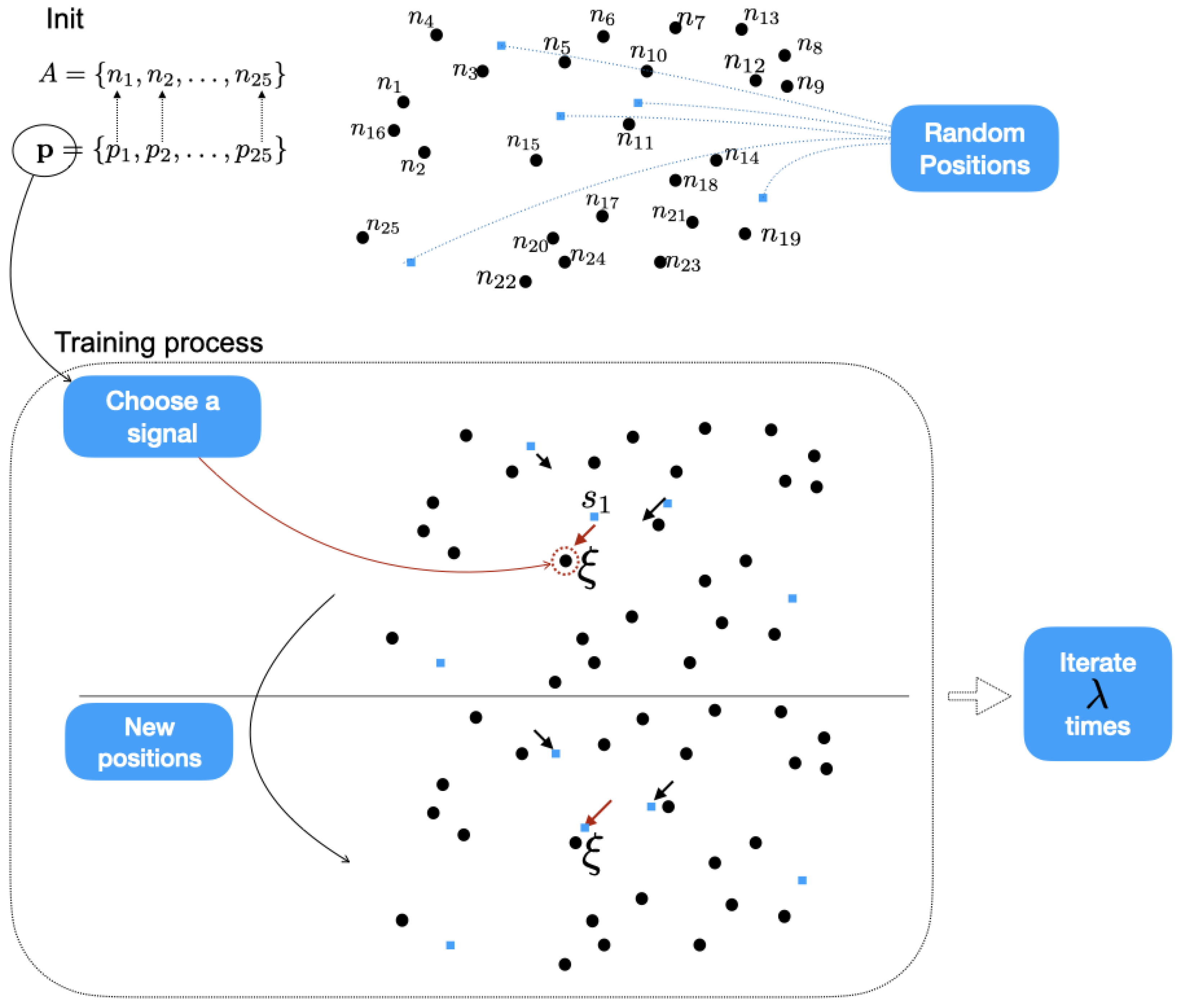
INIT: Start with M points $k_1,k_2,\dots k_M$ at random positions $w_{k_1},w_{k_2},\dots ,w_{k_M}$ in ${\mathrm{R}}^2$. Initialize a local counter to zero for every point. Generate a random point $n_i\in A$ as the input signal $\xi$ taking into account the probability vector ${\mathbf{p}}_i$. Locate the nearest node $s_1\in P$ to the $\xi$. Increase the local counter of the $s_1$ node. Move, concerning the total distance, the position of $s_1$ to $n_i$ by fractions ${ϵ}_{win}$. $$\Delta w_{s_1}={ϵ}_{win}(\xi -w_{s_1}).$$ Determine the second $s_2$ and third $s_3$ nearest nodes to the input signal $\xi$. Move $s_2$ and $s_3$ towards $\xi$ by fractions ${ϵ}_n$ $$\Delta w_{s_2}={ϵ}_n(\xi -w_{s_2}),$$ $$\Delta w_{s_3}={ϵ}_n(\xi -w_{s_3}).$$ Repeat steps 1 to 6 $\lambda$ times, with $\lambda$ being an integer. If the local counter for any $k_i,i=1,2,\dots ,M$ is zero, then remove this node and add a new node between the node with a higher local counter value and any node adjacent to it. If the local counter for every $k_i,i=1,2,\dots ,M$ is greater than zero, then continue and repeat steps 1 to 6. Stop when the maximum number of iterations has been reached.

The basic features of the GNG2D+ algorithm proposed are as follows:

• A probability vector is associated with the initial set of points A. This fact implies that the choice of each signal, in each iteration, is not purely random. If we review the SOM-type algorithms (see the different Appendices), it is characteristic that the initial signal in each iteration is chosen randomly, that is, all the points have the same probability of being chosen as a signal. However, in the proposed algorithm, the probability vector associated with these points is introduced in order to somehow avoid the equal probability of each point being chosen, taking into account any characteristic or weighting that may be considered. In the case that we want randomness in the choice of the points, we assign a constant probability vector.
• To start the construction of the cloud of points, we select M points. This number of points can be parameterized depending on each application. The fact that the algorithm runs every iteration with the same number of final points (the set P) is crucial as it eliminates the need to add or remove nodes, allowing the model to focus on self-learning the topology of the original point set.
• The training process involves three parameters: ${ϵ}_{win}$, ${ϵ}_n$ and $\lambda$. The parameter $\lambda$ ensures that any node in the initial set of random points remains isolated throughout the entire execution of the algorithm. ${ϵ}_{win}$ determines the displacement of the winning node, while ${ϵ}_n$ determines the displacement of the neighboring nodes.

Figure 1 shows a graphical diagram of the initial steps in the execution of the algorithm. A simple example is shown with 25 original points (black dots) and a simplification to 5 final points (blue squares). As can be seen, we initially have the original points, as well as the probability vector associated with them. The 5 points are randomly placed and the training phase of the points begins by “learning” from the original. The signal is chosen and the closest points are determined, to enable the approximation to be performed. This process is iterated a large number of times until the final position of the points is determined.

It is relevant to note that the fact that points have different probabilities of being chosen, based on a weighting vector, can be used to associate each point with a particular characteristic or measure. For instance, if each point belongs to a network and every node has a centrality associated with it, we can use that value as a probability vector so that the most important nodes within the network have a higher probability of being chosen as the initial signal. This fact is very important when working with spatial networks, where the points are defined by their geographical coordinates and where the nodes have a physical and not a virtual meaning.

It should be noted that when comparing the proposed GNG2D+ algorithm with the original GNG2D in Appendix D, the changes are minimal. From a computational point of view, the two main loops of the algorithm that constitute the iterative process are not modified in the new version, so the arithmetic cost of operations is analogous. However, the idea of the model changes radically, since we eliminate the randomness of the original one. The fact that the signals are now chosen in the training process using a probability vector biases the randomness of the original model and allows us to associate a different probability with each point in the original set, depending on the needs of each specific case.

It is appropriate to comment on some aspects relating to the cost and limitations of the algorithm. Common to all SOM-type algorithms is a poor execution time, especially for large-scale problems. See [28] for a detailed description of their efficiency and how we can improve the execution times of these types of algorithms. It should be noted that the incremental nature of the GNG algorithm and the self-organization process of the neurons in it represent the most important part of its computational cost. In our case, the act of initially taking the number of end points of the network and placing them randomly eliminates the incremental nature of the network, which significantly simplifies its cost. In the GNG2D+ algorithm, the most important computational cost comes from the self-organization process of the end nodes, learning the shape of the initial set.

To be more precise, the point of the algorithm that represents a higher computational cost is point 2 relative to the search for the nearest neighbor, which is also the slowest one because it requires iteration over all nodes each time. To compute the nearest node, we use the expression for the Euclidean square distance between two points, $n_1=(x_1,y_1)$ and $n_2=(x_2,y_2)$, which is

$$d{(n_1,n_2)}^2={(x_2-x_1)}^2+{(y_2-y_1)}^2.$$

Note that we carry out this process for each iteration. When the number of points in A is very high, the number of iterations is much higher, so the searching should be based on a more sophisticated algorithm using a supporting structure. For instance, K-d Tree [29] is a well-known structure for the nearest neighbor search based on partitioning of a space into a binary tree using splitting axis-aligned hyperplanes. A K-D Tree is a binary tree in which each node represents a k-dimensional point. Every non-leaf node in the tree acts as a hyperplane, dividing the space into two partitions. This hyperplane is perpendicular to the chosen axis, which is associated with one of the K dimensions.

The fundamental idea that summarizes the GNG2D+ algorithm is that given a set of nodes or points, a simplified dataset is computed in such a way that the new distribution of the generated points maintain the shape or geometry of the original set. In this paper, we will apply this concept to a network simplification problem, using the algorithm to determine the best positions of the simplified set of points so that both networks are geometrically similar.

3. A Case Study: Methodology

The GNG2D algorithm simplifies an original set of points into a simplified one with the same “shape” as the original, allowing the simplification scale to be established in advance. By introducing a set of points as the input, we can use the algorithm to simplify a spatial network where the points are determined by a geographic position. It is enough to take the set A with the geographical coordinates of the nodes of the network as the initial input. The result is a new set of points whose location represents the nodes of the simplified network, with the characteristic that it maintains the topology of the original network.

To check the possibilities of the algorithm in simplifying spatial networks, let us develop, in detail, a case study in which the design of an electric vehicle charging network is proposed based on the spatial network formed by gas stations for combustion vehicles. The geographical area investigated in this study is the Valencian Community (Spain). The objective of this case study is the design and evaluation of an EV charging network in this area as a simplification of the gas station network. The achievement of this objective requires a methodology that can be summarized in three phases: data collection, data processing and application and visualization of the GNG2D+ model.

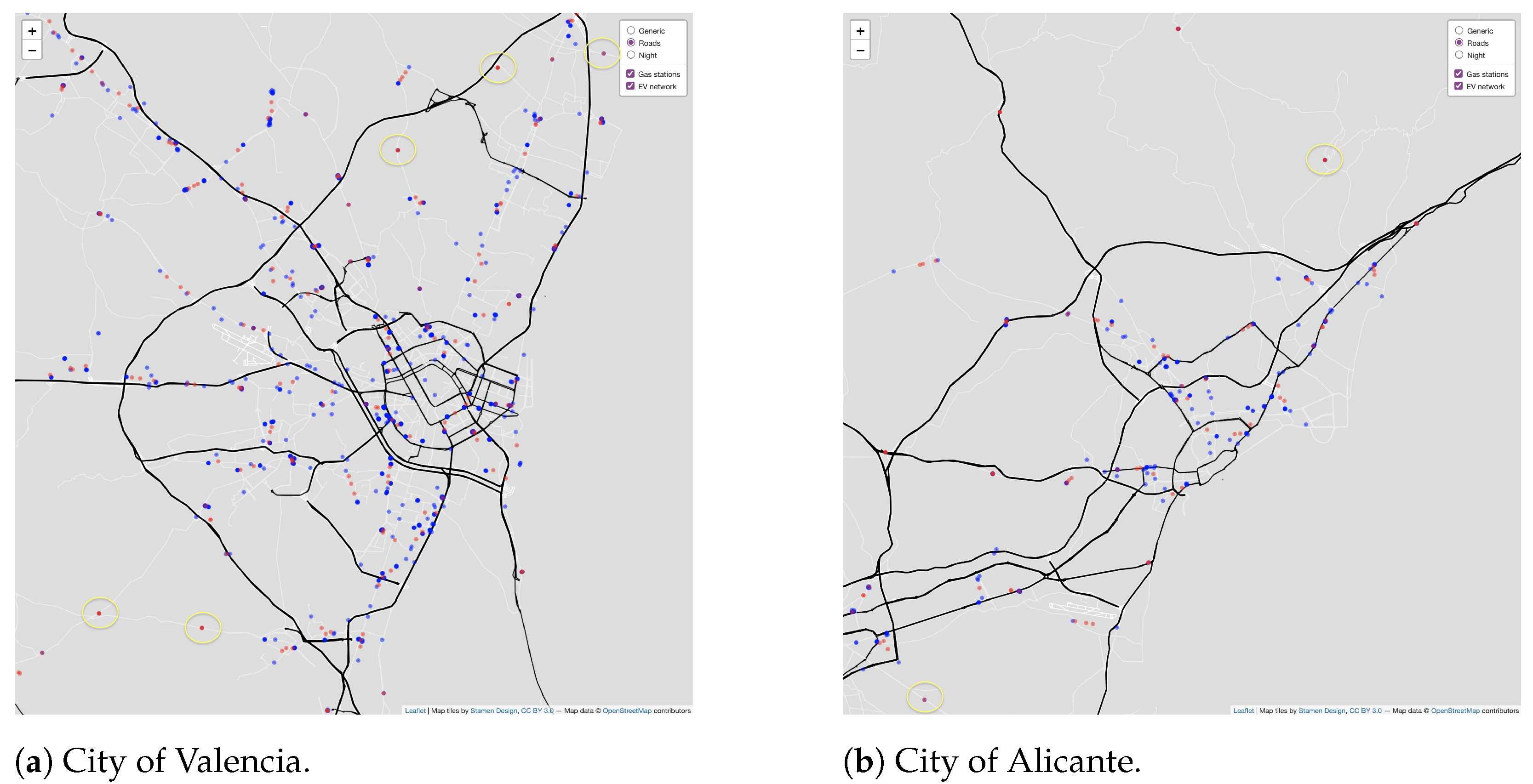
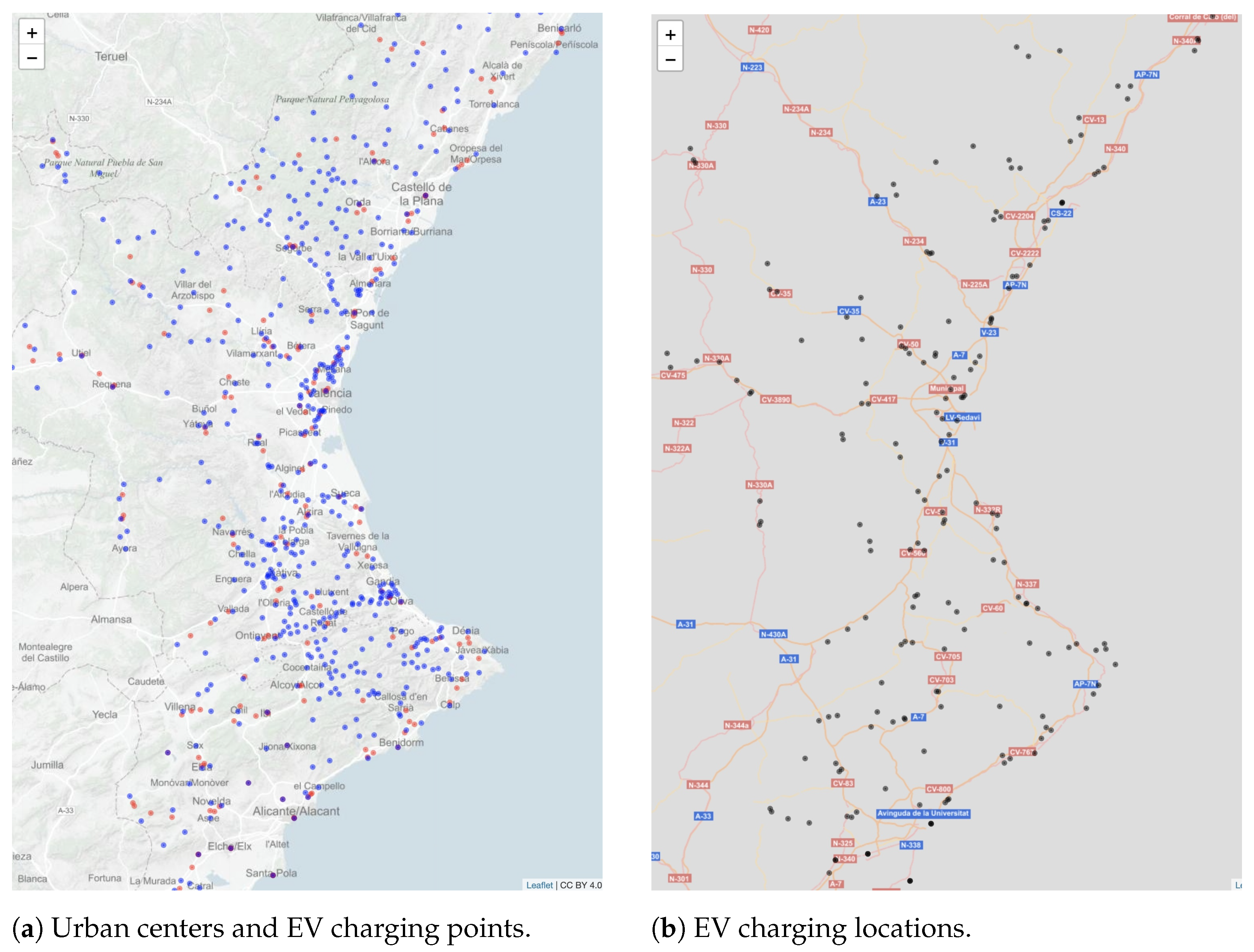
3.1. Data Collection

Three datasets were used to carry out this work, all of them restricted to the geographical area studied:

• Gas stations.
• EV charging points.
• Municipalities and population.

The first part of this work consisted of obtaining the dataset with the locations where there are gas stations for combustion vehicles. The data source used was the OpenStreetMap platform (OSM) (https://www.openstreetmap.org/) (last access 1 February 2024). This is a collaborative project in which a map of the whole world can be edited and used for free. It constitutes a perfect source to obtain data in a simple and free way. However, it is important to recognize that although OpenStreetMap offers advantages in terms of free access and flexibility, it may also have some limitations compared to commercial services such as Google Maps. Some of these limitations can be summarized under two headings:

• Updates and accuracy, since it is the users themselves who provide the information.
• Coverage and accuracy, especially in less favored areas where the community is less participatory.

It should also be noted that even if we filter by city, province or autonomous community, OSM obtains data from a rectangle (called a box) that contains a border. For this reason, it is common to obtain points close to the indicated border that are not inside it.

There are several packages in R that allow us to extract data from OSM. We used osmdata (https://docs.ropensci.org/osmdata/) (last access 1 February 2024). It is an R package that allows access to OpenStreetMap data via the Overpass API, which provides access to custom selected parts of the OSM map data in a read-only format.

As a previous step, the limits of the area of the Valencian Community were obtained and, based on this box, a search for gas stations using the parameters key = ‘amenity’ and value = ‘fuel’ was carried out, using the API. The dataset had 5287 geolocated points with the category of gas stations. Through simple data processing, a table was obtained with the geographic coordinates (longitude–latitude) of each of the points.

Another search was carried out for the points or nodes listed in OSM as charging stations or charging points for electric vehicles, following the parameters or tags key = ‘amenity’ and value = ‘charging_station’. This new dataset will be used later to compare the network generated by the GNG2D+ algorithm with the current existing network.

Finally, data relating to all the municipalities and their populations in the Valencian Community were obtained. These data were obtained from the government agency that governs the territory, more specifically, from the open data portal of the Generalitat Valenciana (https://dadesobertes.gva.es/es/dataset/sanidad-sip-municipios (last access 1 June 2024)). From this portal, we can download the data of the 542 municipalities and their populations (up to 2023). The download format is a compressed file containing the information in a shapefile format.

3.2. Processing Data

Throughout the process of obtaining the data, it was detected, when analyzing the results, that repeated points appeared with the same coordinates or were very close to each other, only several meters apart. This is not surprising and quite expected. Let us think of main or secondary roads where there are gas stations for both directions of travel and they are located opposite each other. Sometimes, two stations were located separated by no more than 20 m. It is also the case that at some stations, different companies share services.

This made it necessary to adjust the data, so clusters where some points were very close to others were unified into a single node or point. The idea was to focus on relevant geographic areas instead of simply counting relevant points. This also reduces noise, facilitates the visualization of the nodes and improves the computational efficiency of the analysis.

Therefore, once the spatial data of gas stations were collected, a data processing step was developed and divided in two steps:

• Elimination of duplicate nodes. The decision to eliminate duplicate nodes by rounding coordinates to three decimal places is based on an important consideration, for the specific purpose of finding areas with gas stations rather than simply counting the number of these points (geographic location is prioritized over quantification).
• Geographic coordinates obtained from the Openstreetmap API must be transformed into UTM coordinates. The reason for this is that geographic coordinates measure degrees, while UTM coordinates allow us to work with distances in meters on the Earth’s surface. Due to the characteristics and meaning of the data used, by working with UTM coordinates, we ensure that distances are measured linearly. So, it will be possible to establish linear distances between points if necessary for our analysis.

Table 1. Details about datasets used.

Dataset	Gas Stations	EV Charging Points	Municipalities
Size	5287	222	542
Date	September 2023	December 2023	2023
Source	OpenStreetMap	OpenStreetMap	ICV
API	Overpass	Overpass	Open Data
Tag	‘fuel’	‘charging_station’
Library	osmdata	osmdata

summarizes the essential details regarding the data tables used, where we have the two datasets obtained (columns 2–4) and the details (rows).

3.3. Application and Visualization of the GNG2D+ Model

The GNG2D+ algorithm was applied to construct a network of EV charging points, taking as a base reference the network of gas stations within the geographical scope of the Valencian Community (Spain). When the problem of designing an efficient network of charging points for electric vehicles was raised, we thought that the starting point could be the network of gas stations. The reason for this is that until a few years ago, practically $100\%$ of the vehicles circulating in urban or interurban areas were diesel- or gasoline-powered vehicles. The network of gas stations, built up over many years, has adapted over time to the needs of people, both for short- and long-distance trips. Therefore, it is reasonable to think that the gas station network is a consolidated and efficient network that provides a good service to everyone.

The particular charging requirements of electric vehicles in terms of charging times, as well as the constant increase in the sales of these vehicles, make the design of a sufficient and efficient charging network an essential aspect in electric mobility. Therefore, it seems a good idea to design the recharging network based on the current network of gas stations. As an example, in France, the government has stated that by 2025, $85\%$ of gas stations on major roads will have fast charging points.

As a consequence of these reflections, in our example, the initial set of points of the GNG2D+ algorithm will be the dataset of gas stations obtained from OSM. Thus, the initial dataset consists of slightly more than 5000 points.

The algorithm was applied by taking a probability vector where each signal is chosen with the same probability at each iteration. Furthermore, the reduction parameter of the final network was taken as $1/5$, which means that we consider building a network of charging points with one fifth of the points representing gas station locations.

When working with spatial networks in which the main feature is geolocation by means of its coordinates, visualization is fundamental. Furthermore, with the objective of improving the efficiency of the network of electric vehicle charging points, it is necessary to pay special attention to essential aspects such as ensuring that the network reaches the majority of the geographic areas and trying to minimize disadvantaged areas in terms of the services offered.

There are numerous packages in R that allow us to build excellent graphs. But there are packages that offer the possibility of creating interactive graphics and maps, where the user interacts directly with the representation itself. Among all the existing ones, we highlight the library leaflet (https://rstudio.github.io/leaflet/articles/leaflet.html (last access 18 September 2024)) both for its simplicity and for the quality and options to generate interactive maps. In addition to providing the aforementioned interactivity, these maps allow stratification, by individual layers, of the various types of geospatial data analyzed, in this particular case, the locations of service stations and charging points. One of the advantages of this library is the ability to select and display these layers selectively on the same map.

4. Numerical Results

4.1. Preliminary Issues

The main task in this section is to analyze and visualize the results obtained by applying the proposed GNG2D+ algorithm to the electric vehicle charging network in the Valencian Community, taking as a reference the existing network of gas stations for combustion vehicles.

The gas station network constitutes a set of points A with which we initialize the GNG2D+ algorithm. Each of these points may be chosen as a signal depending on the probability vector, from which we perform each iteration.

Before analyzing and visualizing the results obtained, it is convenient to visualize the network used as a model or origin to build a simplified network.

Figure 2 shows two maps with the geographical locations of the gas station points in the area evaluated. In Figure 2a, the points are displayed on a generic map with no labels, while in Figure 2b, the points are displayed on a map where the main and secondary roads are highlighted in red color. Remark the correlation between the locations of the gas station points and the road network.

As already mentioned, the reason for taking the gas station network as the basis for the design of our network is due to its characteristics, since it is a network consolidated over many years that offers an adequate service for providing people with mobility. The main characteristic of this network is the high correlation between the location of the fuel outlets and the road network of the territory, as can be seen in Figure 2b.

As expected, remark that there is a direct relationship between higher densities of points in this network and the geographic areas with the highest population density. The geographical area analyzed is made up of three provinces with four major population centers. In addition, high densities of points are observed in the coastal area, as these are areas whose main economic activity is related to leisure and tourism. The “gaps” that appear in several inland areas correspond to rural areas with a low population density.

4.2. Analysis of Numerical Results

For the application of the GNG2D+ algorithm to the set of points of the network of Figure 2, the criterion that all points have the same probability of being chosen as signals in each of the iterations was adopted. Remark that this allows us total flexibility in terms of the size of the simplified network with respect to the original one, which enables us to design the size of the network by first fixing the number of nodes.

Various numerical tests were carried out using the GNG2D+ algorithm for various simplification scales and with different values of the parameters involved. Next,

Table 2. Some data for the parameters involved in the GNG2D+ algorithm.

N	M	Scale	$\mathit{\lambda }$	Iterations	${\mathit{ϵ}}_{\mathit{win}}$	${\mathit{ϵ}}_{\mathit{n}}$	Time
5287	176	$1/30$	$75.000$	100	$0.5$	$0.2$	$40.1$
5287	176	$1/30$	$100.000$	150	$0.5$	$0.2$	$78.1$
5287	264	$1/20$	$75.000$	100	$0.5$	$0.2$	$41.9$
5287	264	$1/20$	$100.000$	100	$0.5$	$0.2$	$63.1$
5287	264	$1/20$	$100.000$	150	$0.5$	$0.2$	$78.2$
5287	528	$1/10$	$75.000$	100	$0.5$	$0.2$	$276.7$
5287	528	$1/10$	$100.000$	150	$0.5$	$0.2$	$306.2$
5287	1057	$1/5$	$100.000$	100	$0.5$	$0.2$	$420.1$
5287	1057	$1/5$	$100.000$	150	$0.5$	$0.2$	$623.8$

summarizes some of the results obtained, as an example.

In Table 2, N represents the number of points of the set A and M the size of the final set after the self-organizing process, while the third column shows the scale of the simplification generated. The parameters in the columns are as follows:

• $\lambda$ is the parameter that sets the number of iterations in the main loop (steps 1–6 of the algorithm).
• Iterations represent the global iterations performed to remove isolated points (step 7).
• ${ϵ}_{win}$ is the displacement of the winning neuron in the self-organizing process.
• ${ϵ}_n$ is the displacement of the nearest neurons in the self-organizing process.

The last column shows the algorithm execution time (in minutes). For measuring the time, we must take into account the following considerations.

• The implementation of the algorithm was not optimized regarding the search for the nearest neighbors.
• Only the execution time of steps 1 to 8 of the algorithm were measured.
• The tests were performed on a computer with an Apple M2 Ultra processor with 64 GB of RAM.

The execution times confirm the comments made in Section 2 on the problems of GNG-type algorithms with respect to the computational cost for large-scale problems. In our case, the number of points is not excessively high, and the objective of this work is to optimize the algorithm but to show the results obtained and the possibilities for this specific problem.

Next, we carry out a basic study of the spatial characteristics of some datasets obtained by the GNG2D+ algorithm. For a more detailed description of the methods used in this analysis and an essential reference in the field of spatial point patterns, see [30].

Three datasets are analyzed with the following characteristics:

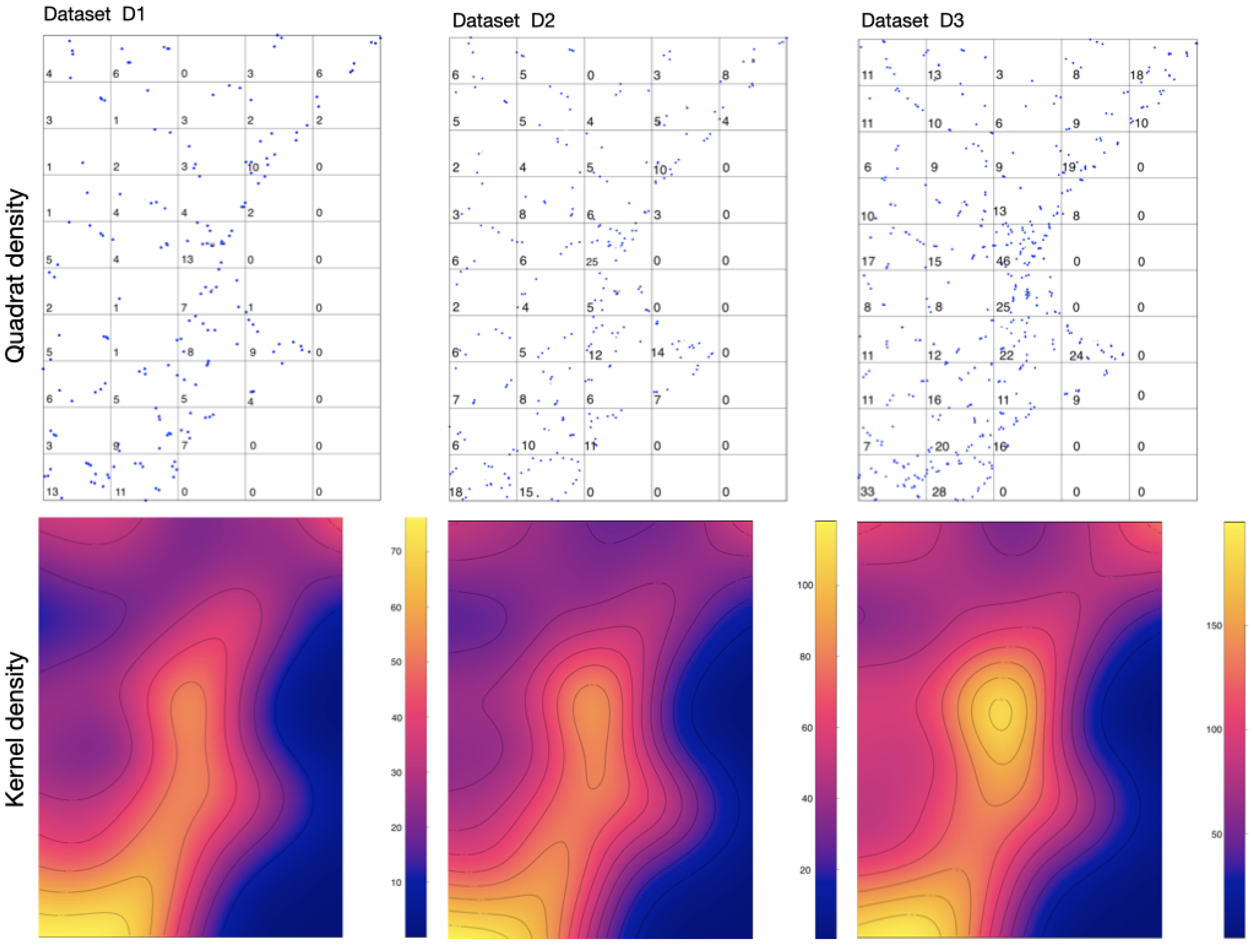
• D1: dataset 1. $M=176$; factor scale: $1/30$.
• D2: dataset 2. $M=264$; factor scale: $1/20$.
• D3: dataset 3. $M=528$; factor scale: $1/10$.

To explore the spatial point patterns in the datasets, there exists a wide variety of models and metrics. They can be classified into two groups: the density-based approach and the distance-based approach.

The density-based technique characterizes the pattern in terms of its distribution as a first-order property of the pattern, while the distance-based approach constitutes a second-order property of the point pattern. The difference is that the first-order property of a pattern concerns itself with the variation in the observations’ densities across a study area; however, in the case of the distance approach, the interest lies in how the points are distributed relative to one another (a second-order property of the point pattern), as opposed to how the points are distributed relative to the study extent.

Regarding the density approach, the following metrics are used:

• Quadrat density: Quadrat counting is a simple way to inspect point pattern data. The window of observation is divided into a grid of rectangular tiles, and the number of data points in each tile is counted.
• Kernel density: Kernel density calculates the magnitude-per-unit area from point or polyline features using a Kernel function to fit a smoothly tapered surface to each point or polyline.

Figure 3 shows graphs summarizing the density metrics for the analyzed datasets. The firs row shows the values of the Quadrat density, for which a $5\times 10$ grid is defined. Approximately, each cell covers a geographic square of about $32.5$ km on each side. The second row shows the Kernel density using a contour plot.

Looking at the images related to the Quadrat and Kernel density, it is confirmed that the intensity in the datasets is inhomogeneous, which was expected. Observing the images related to the Quadrat and Kernel density confirms that the intensity in the datasets is inhomogeneous, which was expected according to the model used to perform the computations. The different scales in the point clouds calculated show a similar pattern, increasing the density values in the mesh in a proportional way. Note the similarity in the contour plots. These similar patterns demonstrate the characteristics and possibilities of the algorithm to learn the shape of the dataset and simplify it while maintaining its topology, even if its scale is modified. The simplifications obtained from the original set of points present a similar geometric shape, which is confirmed by the graphics in Figure 3.

To perform the distance-based analysis, the following functions are used:

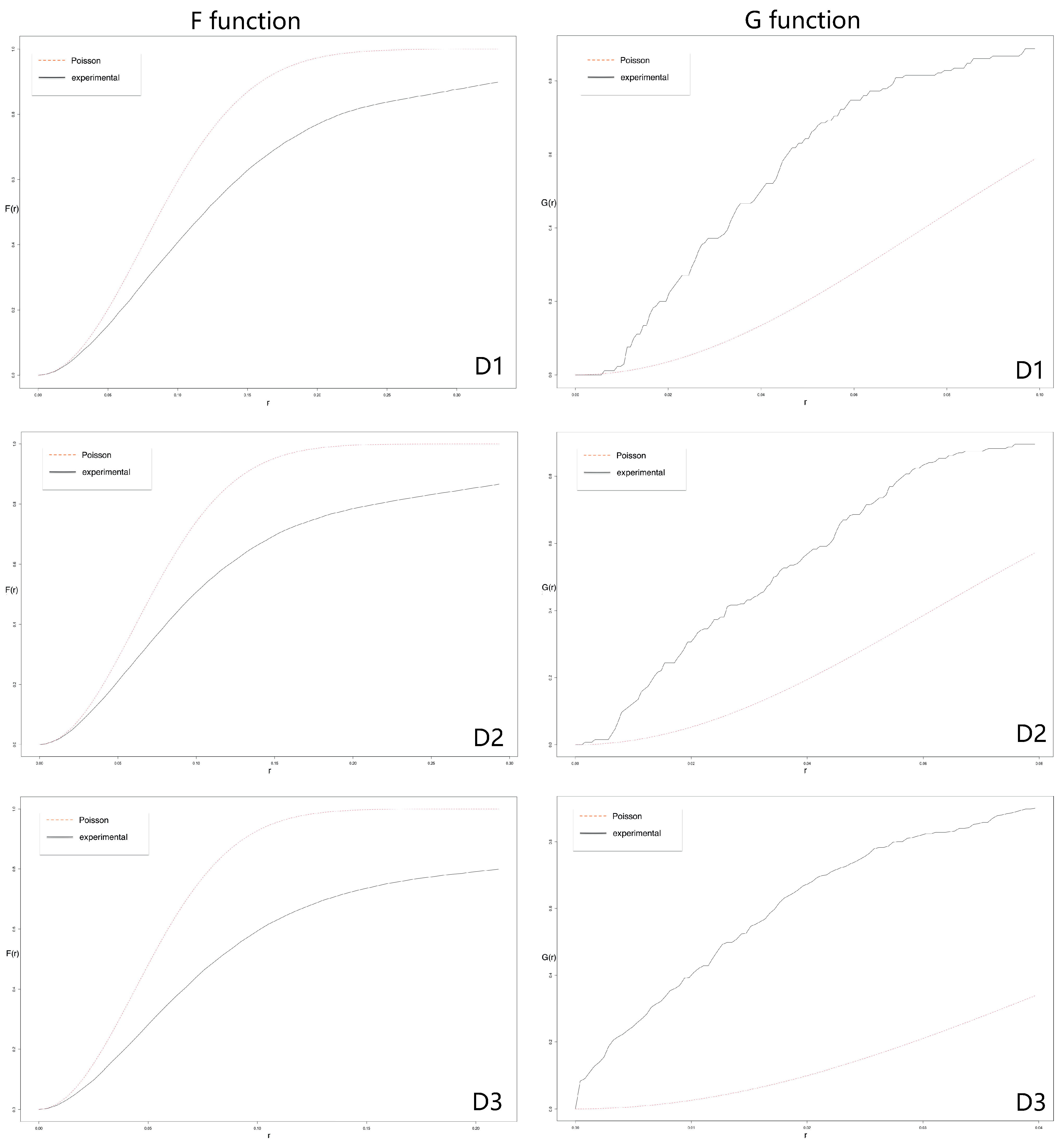
• F: empty space function. The empty space function F of a stationary point process X is the cumulative distribution function of the distance from a fixed point in space to the nearest point of X.
• G: nearest neighbor distance function. The nearest neighbour function G is the cumulative distribution function of the distance from a point of the pattern X to the nearest other point of X.
• K: The K function, also known as Ripley’s K function, is a statistical tool used in spatial analysis to evaluate the distribution of points in a given space. The K function is defined so that $\lambda$K(r) equals the expected number of additional points of X within a distance r of a point of X, where $\lambda$ is the intensity (expected number of points per unit area).
• P: Pair correlation function. The pair correlation function is a modified version of the K function where instead of summing all points within a distance r, points falling within a narrow distance band are summed instead. This function may be seen as the probability of observing a pair of points of the process separated by a distance r, divided by the corresponding probability for a Poisson process.

Figure 4 and Figure 5 display graphs of the distance metrics analyzed, for the three datasets. As can be seen in all the graphics, a comparison is made between the results of the dataset obtained (solid black line) against the result that would give us a uniform Poisson process (dotted red lines). Then, for inferential purposes, the estimates of F, G, K and P are usually compared to their true values for a completely random (Poisson) point process. Both for F and G functions, if X constitutes a uniform Poisson process with intensity $\lambda$, the number of points falling in a set B has a Poisson distribution given by the expression

$$F_{Poisson}\left(r\right)=G_{Poisson}\left(r\right)=1-exp(-\lambda \pi r^2),$$

with r representing the radius of B.

For the K function, the Poisson distribution, regardless of the intensity, is given by

$$K_{Poisson}\left(r\right)=\pi r^2.$$

Looking at these graphs, we detect a common pattern regardless of the scale used. In the case of the empty space function F, the empirical is smaller than the theoretical, while for the nearest neighbor distance function, G and K, the opposite occurs. This suggests that the datasets follow a spatial clustering pattern, far from the randomness assumed by the Poisson process.

Furthermore, when the scale increases and the number of points is larger, the differences between the empirical and theoretical values also become more significant. This is consistent with the geometric arrangement of the original dataset.

4.3. Visualization of the Numerical Results

An essential part of this work is the visual analysis of some of the results obtained. More specifically, we focus on the following simplified scales:

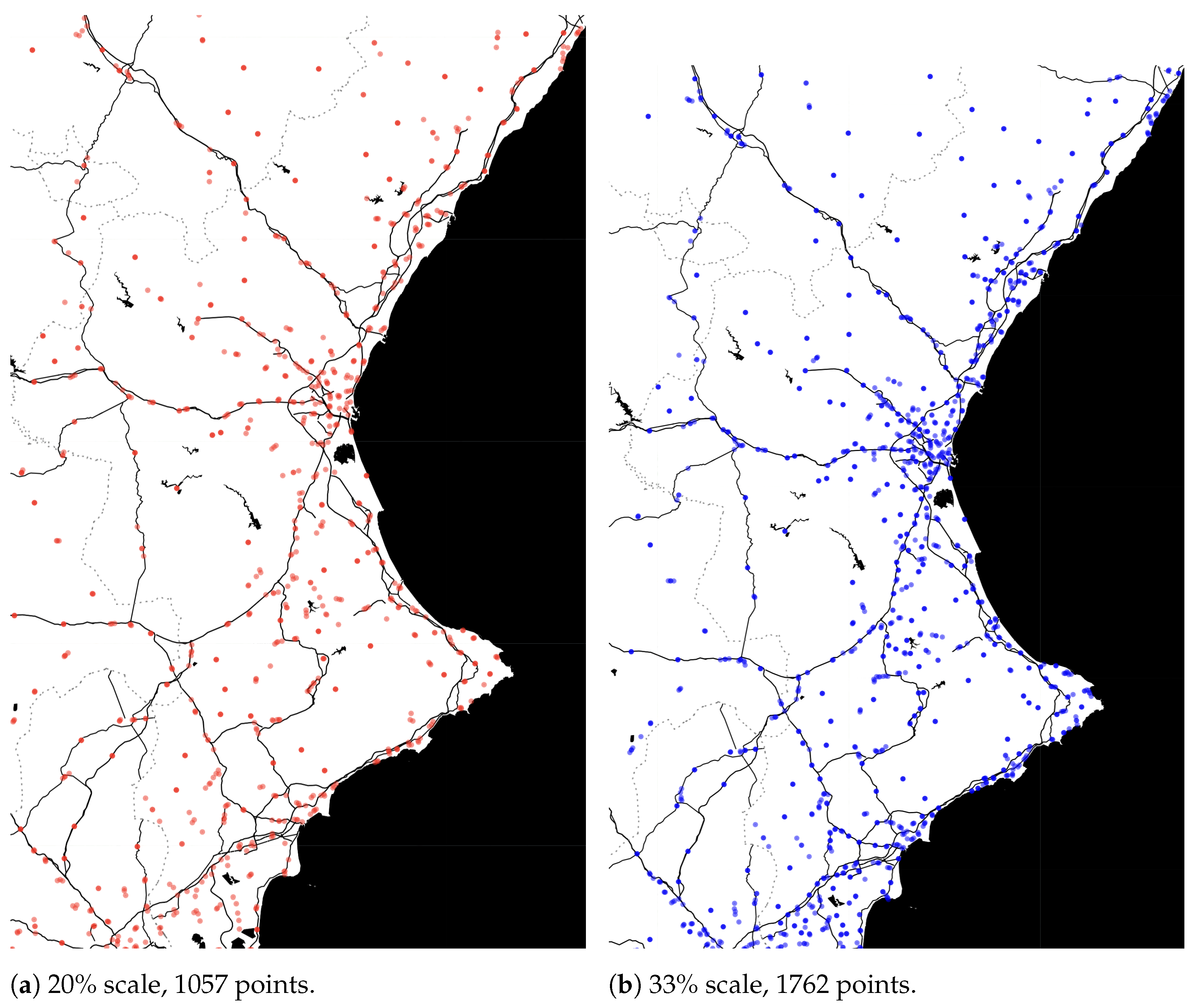
• Initial gas station dataset: 5287 points. Final dataset: $20\%$, i.e., 1057 points.
• Initial gas station dataset: 5287 points. Final dataset: $33\%$, i.e., 1762 points.

Figure 6 shows two maps that reflect the sets of points generated by the GNG2D+ algorithm, for two different sizes of the final set. The map in Figure 6a represents a final dataset of charging stations that is $20\%$ of the size of the original network of gas stations, while in Figure 6b, the final size is $33\%$ of the original network.

Remark that the maps used in these figures are basic and only show the primary and secondary roads, excluding details of a geographical or physical nature. The reason for using this type of map is to better visualize the correlation between the points of the original gas station network and the presence of primary and secondary roads.

It should be noted that algorithms of the GNG2D+ type, as well as algorithms based on the Self-Organizing Map model and its variants, are heuristic. Due to the lack of determinism in the generated networks, they were run several times in order to ensure that the results obtained were similar. The results shown in Figure 6 are similar to those obtained by repeatedly running the algorithm.

For other simplification scales, the conclusions are the same since the maps show us that for different sizes, both datasets present a similar spatial pattern. Although the number of points is increased by $13\%$ in the analyzed cases, the shape and geometry observed are similar. This is important as it reinforces the idea of “learning” from an iterative process. Therefore, the idea of using as the original data set the nodes of a network that we can consider “efficient” for the user, such as the gas station network, means that the final set of points generated by the algorithm also constitutes an efficient network, although simplified with respect to the original. That is, the final dataset inherits the good properties of the original, always speaking in terms of geometry and spatial shapes.

However, the images comparing the original network and the computationally generated one allow us to detect a differential detail between the two. Although the geometry of the constructed network follows that of the matrix network, we clearly notice, regardless of its size, that the network constructed for electric vehicle recharging inserts some points in different areas of the interior of the geographical area studied in which no gas stations are located.

This fact, which might seem to be a conceptual error with respect to the working philosophy, makes the network constructed using the algorithm much more efficient than the original one from the point of view of covering the entire territory and not generating disadvantaged areas in terms of the presence of services. Therefore, the constructed networks have the property of maintaining the topology of the original network covering the whole territory in a more efficient way.

Carrying out a more in-depth investigation into this feature, let us develop a visual comparison between the network of gas stations shown in Figure 2 and the images of the simplified networks shown in Figure 6. The inclusion of new points or nodes in positions where there is not a large concentration of gas stations is perceptible.

In Figure 7, a map of the two most populated cities in the region studied is shown, specifically the cities of Valencia (792,492 inhabitants, in 2022) and Alicante (338,577 inhabitants, in 2022). The images show the best locations for EV charging points in the metropolitan areas of the cities (red color dots), according to the GNG2D+ algorithm, simplifying to $33\%$ of the original dataset. In blue color dots are displayed the gas stations.

By analyzing a much smaller area, the same behavior is detected as on a larger scale. Both point distributions present a similar configuration in terms of their geometry, although some points are also located in places where there are no nodes of the original network.

The construction of the network developed so far has been purely algorithmic; an algorithm has determined the best positions of a set of points following a geometrical structure similar to a given original network. However, the points of the constructed network have a physical meaning, as they represent charging stations for people traveling with electric vehicles. Therefore, when constructing such a network, it must be taken into account that the ultimate purpose of the network is to provide a service to people. This leads us to consider the need to relate the positions obtained to population density. It makes no sense to place a large number of service stations in areas that are not populated or where no one is going to pass through. Resource optimization leads us to try to somehow relate services to population density. We can address this issue by reusing the GNG2D+ algorithm with the following initial parameters:

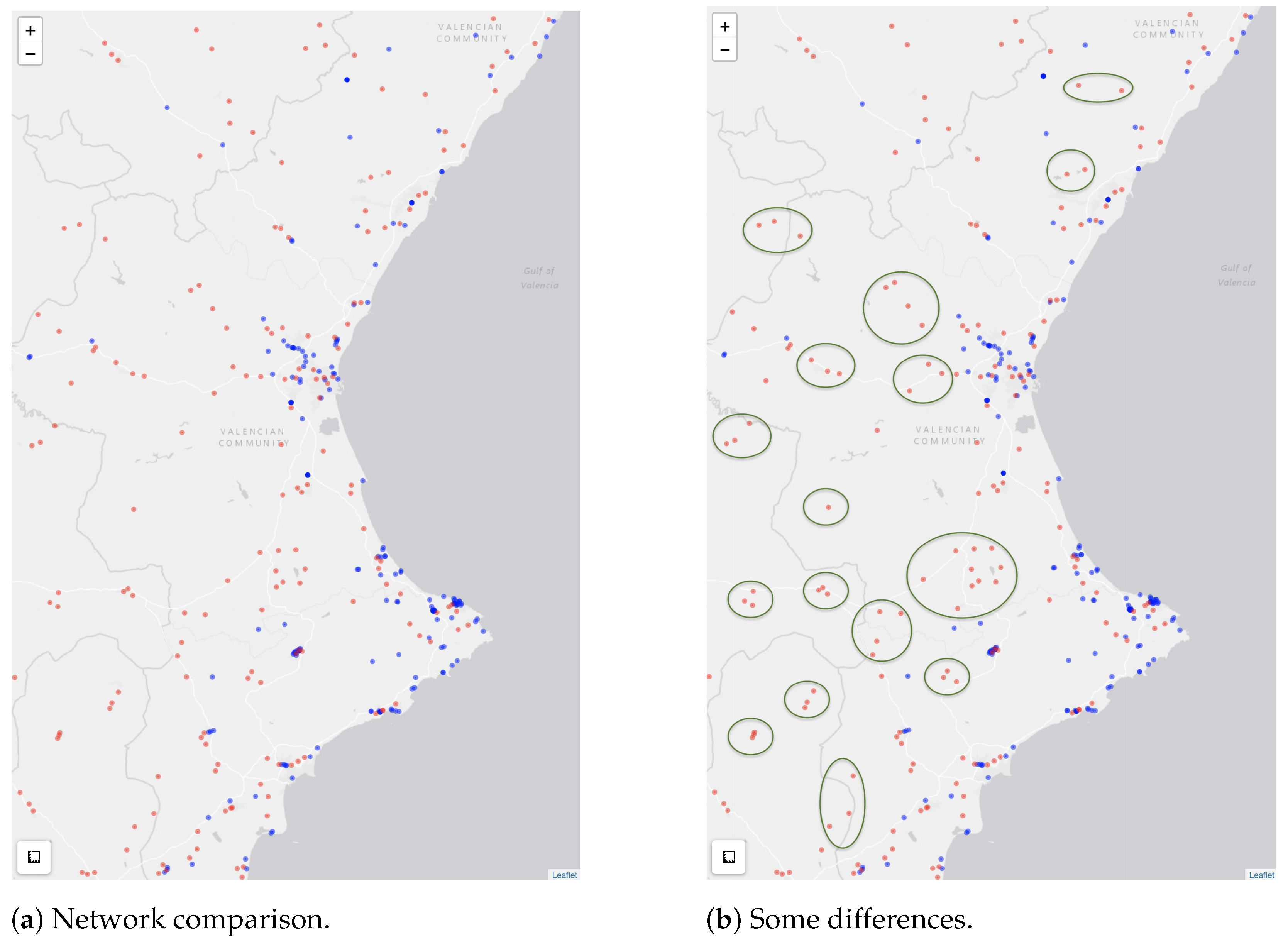
• The original network used and that introduced as an input parameter will be formed by the urban centers of the geographical area studied.
• The probability vector p associated with this dataset will be the normalized population density vector of each urban center.
• The initial set of points, randomly generated at the beginning of the algorithm, is replaced by the final set of points obtained in the first execution of the algorithm, represented in Figure 6.

With these modifications, the GNG2D+ algorithm is executed, with the aim of obtaining a final set of points that approximate areas with a given population density. This allows us to reinforce the relationship between service points and urban presence. In addition, by introducing a probability vector based on the number of inhabitants of each urban nucleus, we are giving more importance to the location of services in more densely populated areas. The results obtained after rerunning the algorithm with the modifications and initial values are shown in Figure 8.

In Figure 8a, we present the calculated network of recharging points (red color) by means of the GNG2D+ algorithm and the points where there are urban centers (blue color). As expected, the points generated from the algorithm are close to urban centers, especially those that are more populated. Figure 8b shows the points generated by the algorithm and their locations based on the map of main and secondary roads in the geographical area studied. We visually check the correlation with the roads again, especially on the main roads. Therefore, a location for the points or nodes of the network that is close to urban centers and main roads is obtained, representing two essential characteristics that may be associated with the constructed network.

A recharging network built with the GNG2D+ algorithm taking the gas station network as a reference has been designed. The question is whether or not the networks generated by the GNG2D+ algorithm are similar to the current network of recharging points existing in this region.

In order to carry out this comparison, we first obtained the current data of the existing public recharging points in the Valencian Community. Public charging points were obtained by OSM through the library osmdata, following a process similar to the one we followed to obtain the data on gas stations. This library provides a simple way to download and import Open Street Map data as simple features (sf) or spatial objects (sp) into R. The data were extracted from the Overpass API, which is a read-only API that extracts selected custom parts of OSM data.

Remark that, regardless of the filter used, OSM obtains the data from a rectangle containing a boundary. For this reason, it is common to obtain points close to the boundary that are not inside it.

In order to develop a comparison while taking a similar number of points in both networks, the GNG2D+ algorithm was run while taking a fraction of exactly $1/25$ of the original gas station network. Therefore, the number of points generated by the algorithm is 211 points instead of the 5275 points generated by the original dataset.

In Figure 9 two maps are displayed comparing the currently existing electric vehicle charging network (September 2023) and the network generated using the neural network algorithm. Figure 9a shows the location of the points generated by the algorithm (red dots) versus the location of the points in the current network (blue dots). Likewise Figure 9b shows some geographic areas where the algorithm provides locations and there is a gap in the current network.

These examples demonstrate that the algorithm suggests locations of a dataset and learns the shape of the original network; however, it goes further since it “fills” the space more efficiently and covers the whole territory more efficiently.

5. Discussion

Self-Organizing Maps algorithms, specifically those based on the Growing Neural Gas model, are able to learn the shape of a set of points to generate a simplification of it whose main feature is that it maintains the geometry of the original set. Taking as a basis the idea of the unsupervised learning growth process, which is based the GNG algorithm, a new algorithm GNG2D+ is proposed. The main feature of this model is that it is able to simplify an original dataset into another simplified dataset while maintaining the original topology with a similar geometric shape.

Taking the nodes of a spatial network as the original data set, the model can be applied to build simplified networks with respect to the original so that they maintain a similar geometry, reducing the density of the network. Taking this idea as a basis, as well as the learning capability of the GNG2D+ algorithm, a real example is developed, consisting of the design and evaluation of a network of electric vehicle charging points in the geographical area of the Valencian Community, in Spain.

For the design of the network, the nodes of the petrol station network are taken as the original dataset, since this constitutes an efficient service network for users of combustion vehicles. Simplified datasets are calculated at 20 and 30 percent of the original network. The results show the capabilities of the algorithm to simplify sets of points while maintaining the original topology.

In order to relate the location of the final points to the presence of urban centers, a second step is carried out in which the neural network algorithm is executed, now taking as the initial network the towns and cities of the region and approximating the points to the inhabited areas. The results and the visual analysis of them show us a final network that maintains the shape of the network of service stations and that presents a high correlation with the urban centers and with the main road network. Finally, a comparison is made between the network generated with the neural network algorithm and the current existing network in the analyzed area, showing the differences between the two.

6. Conclusions

The main idea of this work is to evaluate the usefulness of an unsupervised learning neural network algorithm, based on the Growing Neural Gas algorithm, for the design of a spatial network for recharging electric vehicles in a given geographic area. This network is built using the existing gasoline network as a reference because this network has proven its efficiency and was built based on the needs of users who make trips. In addition, when comparing with the charging points in this network with the actual existing EV charging points, a simple visual analysis of the final network obtained allows to detect possible deficiencies in isolated areas or where resources are insufficient.

In future work, we will perform various analyses, such as a comparison of the results obtained for the GNG2D+ algorithm with other alternative methods. Another issue to be studied is the possible optimization of the implementation of the algorithm by improving its scalability for large sets of points.

References

- Rafaj, P.; Kiesewetter, G.; Gül, T.; Schöpp, W.; Cofala, J.; Klimont, Z.; Purohit, P.; Heyes, C.; Amann, M.; Borken-Kleefeld, J.; et al. Outlook for clean air in the context of sustainable development goals. Glob. Environ. Change 2018, 53, 1–11. [Google Scholar] [CrossRef]
- Rohde, R.A.; Muller, R.A. Air Pollution in China: Mapping of Concentrations and Sources. PLoS ONE 2015, 10, e0135749. [Google Scholar] [CrossRef] [PubMed]
- Ruggieri, R.; Ruggeri, M.; Vinci, G.; Poponi, S. Electric Mobility in a Smart City: European Overview. Energies 2021, 14, 315. [Google Scholar] [CrossRef]
- Oladunni, O.J.; Mpofu, K.; Olanrewaju, O.A. Greenhouse gas emissions and its driving forces in the transport sector of South Africa. Energy Rep. 2022, 8, 2052–2061. [Google Scholar] [CrossRef]
- Zuo, J.; Zhong, Y.; Yang, Y.; Fu, C.; He, X.; Bao, B.; Qian, F. Analysis of carbon emission, carbon displacement and heterogeneity of Guangdong power industry. Energy Rep. 2022, 8, 438–450. [Google Scholar] [CrossRef]
- Morfeldt, J.; Davidsson Kurland, S.; Johansson, D.J. Carbon footprint impacts of banning cars with internal combustion engines. Transp. Res. Part D Transp. Environ. 2021, 95, 102807. [Google Scholar] [CrossRef]
- Tran, M.K.; Bhatti, A.; Vrolyk, R.; Wong, D.; Panchal, S.; Fowler, M.; Fraser, R. A Review of Range Extenders in Battery Electric Vehicles: Current Progress and Future Perspectives. World Electr. Veh. J. 2021, 12, 54. [Google Scholar] [CrossRef]
- Hossain Lipu, M.S.; Miah, M.S.; Ansari, S.; Wali, S.B.; Jamal, T.; Elavarasan, R.M.; Kumar, S.; Naushad Ali, M.M.; Sarker, M.R.; Aljanad, A.; et al. Smart Battery Management Technology in Electric Vehicle Applications: Analytical and Technical Assessment toward Emerging Future Directions. Batteries 2022, 8, 219. [Google Scholar] [CrossRef]
- Biresselioglu, M.E.; Demirbag Kaplan, M.; Yilmaz, B.K. Electric mobility in Europe: A comprehensive review of motivators and barriers in decision making processes. Transp. Res. Part A Policy Pract. 2018, 109, 1–13. [Google Scholar] [CrossRef]
- Ray, S.; Kasturi, K.; Patnaik, S.; Nayak, M.R. Review of electric vehicles integration impacts in distribution networks: Placement, charging/discharging strategies, objectives and optimisation models. J. Energy Storage 2023, 72, 108672. [Google Scholar] [CrossRef]
- Campaña, M.; Inga, E. Optimal deployment of fast-charging stations for electric vehicles considering the sizing of the electrical distribution network and traffic condition. Energy Rep. 2023, 9, 5246–5268. [Google Scholar] [CrossRef]
- Chaturvedi, B.; Nautiyal, A.; Kandpal, T.; Yaqoot, M. Projected transition to electric vehicles in India and its impact on stakeholders. Energy Sustain. Dev. 2022, 66, 189–200. [Google Scholar] [CrossRef]
- Cui, D.; Wang, Z.; Liu, P.; Wang, S.; Dorrell, D.G.; Li, X.; Zhan, W. Operation optimization approaches of electric vehicle battery swapping and charging station: A literature review. Energy 2023, 263, 126095. [Google Scholar] [CrossRef]
- Zhuang, R.; Jiang, D.; Wang, Y. An approach to optimize building area ratios scheme of urban complex in different climatic conditions based on comprehensive energy performance evaluation. Appl. Energy 2023, 329, 120309. [Google Scholar] [CrossRef]
- Tsoi, K.H.; Loo, B.P.; Tal, G.; Sperling, D. Pioneers of electric mobility: Lessons about transport decarbonisation from two bay areas. J. Clean. Prod. 2022, 330, 129866. [Google Scholar] [CrossRef]
- Lu, G.; Zhou, X.; Mahmoudi, M.; Shi, T.; Peng, Q. Optimizing resource recharging location-routing plans: A resource-space-time network modeling framework for railway locomotive refueling applications. Comput. Ind. Eng. 2019, 127, 1241–1258. [Google Scholar] [CrossRef]
- Zhang, X.; Rey, D.; Waller, S.T.; Chen, N. Range-Constrained Traffic Assignment with Multi-Modal Recharge for Electric Vehicles. Netw. Spat. Econ. 2019, 19, 633–668. [Google Scholar] [CrossRef]
- Almansour, M. Electric vehicles (EV) and sustainability: Consumer response to twin transition, the role of e-businesses and digital marketing. Technol. Soc. 2022, 71, 102135. [Google Scholar] [CrossRef]
- Erbaş, M.; Kabak, M.; Özceylan, E.; Çetinkaya, C. Optimal siting of electric vehicle charging stations: A GIS-based fuzzy Multi-Criteria Decision Analysis. Energy 2018, 163, 1017–1031. [Google Scholar] [CrossRef]
- Griffith, D.A.; Chun, Y.; Kim, H. Spatial autocorrelation informed approaches to solving location–allocation problems. Spat. Stat. 2022, 50, 100612. [Google Scholar] [CrossRef]
- Kohonen, T. Self-organized formation of topologically correct feature maps. Biol. Cybern. 1982, 43, 59–69. [Google Scholar] [CrossRef]
- Martinetz, T.; Schulten, K. A “neural-gas” network learns topologies. Artif. Neural Netw. 1991, 1, 397–402. [Google Scholar]
- Fritzke, B. Growing Cell Structures—A Self-organizing Network in k Dimensions. In Artificial Neural Networks; Aleksander, I., Taylor, J., Eds.; North-Holland: Amsterdam, The Netherlands, 1992; pp. 1051–1056. [Google Scholar] [CrossRef]
- Licen, S.; Astel, A.; Tsakovski, S. Self-organizing map algorithm for assessing spatial and temporal patterns of pollutants in environmental compartments: A review. Sci. Total Environ. 2023, 878, 163084. [Google Scholar] [CrossRef]
- Tortosa, L.; Vicent, J.; Zamora, A. A model to simplify 2D triangle meshes with irregular shapes. Appl. Math. Comput. 2010, 216, 2937–2946. [Google Scholar] [CrossRef]
- Jose, L.; Oliver, L.T.; Vicent, J.F. A neural network model to develop actions in urban complex systems represented by 2D meshes. Int. J. Comput. Math. 2011, 88, 3361–3379. [Google Scholar] [CrossRef]
- Jose, L.; Oliver, L.T.; Vicent, J.F. An application of a self-organizing model to the design of urban transport networks. J. Intell. Fuzzy Syst. 2011, 22, 141–154. [Google Scholar]
- Fišer, D.; Faigl, J.; Kulich, M. Growing neural gas efficiently. Neurocomputing 2013, 104, 72–82. [Google Scholar] [CrossRef]
- Bentley, J.L. Multidimensional binary search trees used for associative searching. Commun. ACM 1975, 18, 509–517. [Google Scholar] [CrossRef]
- Baddeley, A.; Rubak, E.; Turner, R. Spatial Point Patterns: Methodology and Applications with R; Chapman and Hall/CRC Press: London, UK, 2015. [Google Scholar]