A Comparative View of Becker, Lomnitz, and Lambert Linear Viscoelastic Models

Abstract

We compare the classical viscoelastic models due to Becker and Lomnitz with respect to a recent viscoelastic model based on the Lambert W function. We take advantage of this comparison to derive new analytical expressions for the relaxation spectrum in the Becker and Lomnitz models, as well as novel integral representations for the retardation and relaxation spectra in the Lambert model. In order to derive these analytical expressions, we have used the analytical properties of the exponential integral and the Lambert W function, as well as the Titchmarsh’s inversion formula of the Stieltjes transform. In addition, we prove some interesting inequalities by comparing the different models considered, as well as the non-negativity of the retardation and relaxation spectral functions. This means that the complete monotonicity of the rate of creep and the relaxation functions is satisfied, as required by the classical theory of linear viscoelasticity.

1. Introduction

According to the theory of linear viscoelasticity, a material under a unidirectional loading can be represented as a linear system where either stress, $\sigma \left(t\right)$, or strain, $ϵ\left(t\right)$, serve as input (excitation function) or output (response function), respectively. Considering that stress and strain are scaled with respect to suitable reference states, the input in a creep test is $\sigma \left(t\right)=\theta \left(t\right)$, while in a relaxation test, it is $ϵ\left(t\right)=\theta \left(t\right)$, where $\theta \left(t\right)$ denotes the Heaviside function. The corresponding outputs are described by time-dependent material functions. For the creep test, the output is defined as the creep compliance $J\left(t\right)=ϵ\left(t\right)$, and for the relaxation test, the output is defined as the relaxation modulus $G\left(t\right)=\sigma \left(t\right)$. Experimentally, $J\left(t\right)$ is always non-decreasing and non-negative, while $G\left(t\right)$ is non-increasing and non-negative.

According to Gross [1], it is quite common to require the existence of non-negative retardation $R_{ϵ}\left(\tau \right)$ and relaxation $R_{\sigma }\left(\tau \right)$ spectra for the material functions $J\left(t\right)$ and $G\left(t\right)$, respectively. These functions are defined as ([2], Equation (2.30b))

$$\begin{array}{ccc}\hfill J\left(t\right)& =& a{\int }_0^{\infty }{R}_{ϵ}\left(\tau \right)\left(1-e^{-t/\tau }\right)d\tau ,\hfill \end{array}$$

(1)

$$\begin{array}{ccc}\hfill G\left(t\right)& =& b{\int }_0^{\infty }{R}_{\sigma }\left(\tau \right)e^{-t/\tau }d\tau .\hfill \end{array}$$

(2)

From a mathematical point of view, these requirements are equivalent to state that $J\left(t\right)$ is a Bernstein function and that $G\left(t\right)$ is a completely monotone (CM) function. We recall that the derivative of a Bernstein function is a CM function, and that any CM function can be expressed as the Laplace transform of a non-negative function, that we refer to as the corresponding spectral function or simply spectrum. For details on Bernstein and CM functions, we refer the reader to the excellent treatise by Schilling et al. [3].

In order to calculate $R_{ϵ}\left(\tau \right)$ and $R_{\sigma }\left(\tau \right)$ from $J\left(t\right)$ and $G\left(t\right)$, Gross introduced the frequency spectral functions $S_{ϵ}\left(\omega \right)$ and $S_{\sigma }\left(\omega \right)$, defined as ([2], Equation (2.32))

$$\begin{array}{ccc}\hfill S_{ϵ}\left(\omega \right)& =& a{\displaystyle \frac{R_{ϵ}\left(\frac{1}{\omega }\right)}{{\omega }^2}},\hfill \end{array}$$

(3)

$$\begin{array}{ccc}\hfill S_{\sigma }\left(\omega \right)& =& b{\displaystyle \frac{R_{\sigma }\left(\frac{1}{\omega }\right)}{{\omega }^2}},\hfill \end{array}$$

(4)

where $\omega ={\displaystyle \frac{1}{\tau }}$. Therefore, taking the scaling factors $a=b=1$, we have

$$R_{ϵ}\left(\tau \right)={\displaystyle \frac{1}{{\tau }^2}}{S}_{ϵ}\left({\displaystyle \frac{1}{\tau }}\right),$$

(5)

and

$$R_{\sigma }\left(\tau \right)={\displaystyle \frac{1}{{\tau }^2}}{S}_{\sigma }\left({\displaystyle \frac{1}{\tau }}\right).$$

(6)

In the existing literature, many viscoelastic models for the material functions $J\left(t\right)$ and $G\left(t\right)$ have been proposed in order to describe the experimental evidence. The first pioneer to work on linear viscoelastic models was Richard Becker (1887–1955). In 1925, Becker introduced a creep law to deal with the deformation of particular viscoelastic and plastic bodies on the basis of empirical arguments [4]. This creep law has found applications in ferromagnetism [5], and in dielectrics [1]. This model has been generalized in [6] by using a generalization of the exponential integral based on the Mittag–Leffler function. In 1956, Cinna Lomnitz (1925–2016) introduced a logarithmic creep law to treat the creep behaviour of igneous rocks [7]. This law was also used by Lomnitz to explain the damping of the free core nutation of the Earth [8], and the behavior of seismic S-waves [9]. In order to generalize the Lomnitz model, Harold Jeffreys introduced a new model depending on a parameter $\alpha \in \left[0,1\right]$ in 1958 [10]. When $\alpha \to 0$, the Jeffreys model is reduced to the Lomnitz model. In ([2], Section 2.10.1), the Jeffreys model is extended to negative values of $\alpha$. Very recently, the authors have proposed a new model based on the Lambert W function [11]. In order to evaluate the principal features of this new model, the main aim of the paper is to compare it with respect to the Becker and Lomnitz models, since these classical models have several applications and generalizations in the literature.

This paper is organized as follows. In Section 2, we introduce some basic concepts of linear viscoelasticity that will be used throughout the article. We present the dimensionless relaxation modulus $\varphi \left(t\right)$, as well as the frequency spectral functions $S_{ϵ}\left(\omega \right)$ and $S_{\sigma }\left(\omega \right)$ in terms of the Laplace transform. Section 3, Section 4 and Section 5 are devoted to the derivation of analytical expressions for $\varphi \left(t\right)$, as well as $R_{ϵ}\left(\tau \right)$ and $R_{\sigma }\left(\tau \right)$ in Becker, Lomnitz, and Lambert models, respectively. As far as the authors are aware, the closed-form expressions found for $R_{\sigma }\left(\tau \right)$ in Becker and Lomnitz models are novel. Also, the integral expressions found for $R_{ϵ}\left(\tau \right)$ and $R_{\sigma }\left(\tau \right)$ in the Lambert model are also novel. In Section 6, we graphically compare the models considered here. Finally, we present our conclusions in Section 7.

2. Essentials of Linear Viscoelasticity

In Earth rheology, the law of creep is usually written as

$$J\left(t\right)=J_U\left[1+q\psi \left(t\right)\right],t\ge 0,$$

(7)

where t is time, $J_U$ is the unrelaxed compliance, q is a positive dimensionless material constant, and $\psi \left(t\right)$ is the dimensionless creep function. Note that the scaling factor q takes into account the effect of different types of materials following the same creep model, i.e., the same dimensionless creep function $\psi \left(t\right)$. Since $J\left(0\right)=J_U$, we have

$$\psi \left(0\right)=0.$$

The dimensionless relaxation function is defined as

$$\varphi \left(t\right)=J_{U}G\left(t\right),$$

where $G\left(t\right)$ is the relaxation modulus. Note that $J_U$ acts as a scaling factor for the dimensionless relaxation modulus $\varphi \left(t\right)$. This dimensionless relaxation function obeys the Volterra integral equation ([2], Equation (2.89)):

$$\varphi \left(t\right)=1-q{\int }_0^t{\psi }^{\prime }\left(u\right)\varphi \left(t-u\right)du.$$

(8)

From (8), we have

$$\varphi \left(0\right)=1.$$

(9)

Assuming $q=1$, the solution of (8) is (see Appendix A)

$$\varphi \left(t\right)={\mathcal{L}}^{-1}\left[{\displaystyle \frac{1}{s\left(1+\mathcal{L}\left[{\psi }^{\prime }\left(t\right);s\right]\right)}};t\right],$$

(10)

where $\mathcal{L}\left[f\left(t\right);s\right]={\int }_0^{\infty }{e}^{-st}f\left(t\right)dt$ denotes the Laplace transform of the function $f\left(t\right)$ and ${\mathcal{L}}^{-1}\left[f\left(t\right);s\right]$ is its inverse Laplace transform.

Frequency Spectral Functions

From the definitions given in (1)–(4), we can derive that the creep rate $J^{\prime }\left(t\right)$ can be expressed in terms of the frequency spectral function $S_{ϵ}\left(\omega \right)$ as (see ([2], Equation (2.35)))

$$J^{\prime }\left(t\right)=\mathcal{L}\left[\omega S_{ϵ}\left(\omega \right);t\right],$$

and the relaxation modulus rate $G^{\prime }\left(t\right)$ can be expressed in terms of the frequency spectral function $S_{\sigma }\left(\omega \right)$ as

$$G^{\prime }\left(t\right)=-\mathcal{L}\left[\omega S_{\sigma }\left(\omega \right);t\right].$$

(11)

On the one hand, taking the scaling factors $q=1$ and $J_U=1$, and differentiating in (7), we have that

$${\psi }^{\prime }\left(t\right)=\mathcal{L}\left[\omega S_{ϵ}\left(\omega \right);t\right];$$

thus,

$$\mathcal{L}\left[{\psi }^{\prime }\left(t\right);s\right]=\mathcal{S}\left[\omega S_{ϵ}\left(\omega \right);s\right],$$

where $\mathcal{S}\left[f\left(t\right);s\right]={\int }_0^{\infty }{\displaystyle \frac{f\left(t\right)}{t+s}}dt$ denotes the Stieltjes transform ([12], Equation (1.14.47)). Applying Titchmarsh’s inversion formula ([13], Section 3.3), we obtain

$$S_{ϵ}\left(\omega \right)={\displaystyle \frac{1}{\pi \omega }}\mathrm{Im}\mathcal{L}{\left[{\psi }^{\prime }\left(t\right);s\right]}_{s=\omega e^{-i\pi }}.$$

(12)

On the other hand, taking again $J_U=1$ in (7), from (11), we have

$${\varphi }^{\prime }\left(t\right)=G^{\prime }\left(t\right)=-\mathcal{L}\left[\omega S_{\sigma }\left(\omega \right);t\right];$$

thus,

$$\mathcal{L}\left[{\varphi }^{\prime }\left(t\right);s\right]=-\mathcal{S}\left[\omega S_{\sigma }\left(\omega \right);s\right].$$

(13)

However,

$$\mathcal{L}\left[{\varphi }^{\prime }\left(t\right);s\right]=s\mathcal{L}\left[\varphi \left(t\right);s\right]-\varphi \left(0\right);$$

therefore, according to (9) and (13), we obtain

$$1-s\mathcal{L}\left[\varphi \left(t\right);s\right]=\mathcal{S}\left[\omega S_{\sigma }\left(\omega \right);s\right].$$

Apply Titchmarsh’s inversion formula again to arrive at

$$\begin{array}{ccc}\hfill S_{\sigma }\left(\omega \right)& =& {\displaystyle \frac{1}{\pi \omega }}\mathrm{Im}{\left\{1-s\mathcal{L}\left[\varphi \left(t\right);s\right]\right\}}_{s=\omega e^{-i\pi }}\hfill \\ & =& -{\displaystyle \frac{1}{\pi \omega }}\mathrm{Im}{\left\{s\mathcal{L}\left[\varphi \left(t\right);s\right]\right\}}_{s=\omega e^{-i\pi }}.\hfill \end{array}$$

Finally, according to (10), we have

$$S_{\sigma }\left(\omega \right)=-{\displaystyle \frac{1}{\pi \omega }}\mathrm{Im}{\left\{{\displaystyle \frac{1}{1+\mathcal{L}\left[{\psi }^{\prime }\left(t\right);s\right]}}\right\}}_{s=\omega e^{-i\pi }}.$$

(14)

As pointed out in (5) and (6), the retardation $R_{ϵ}\left(\tau \right)$ and relaxation $R_{\sigma }\left(\tau \right)$ spectra are obtained from the frequency spectral functions $S_{ϵ}\left(\omega \right)$ and $S_{\sigma }\left(\omega \right)$ by considering $\omega ={\displaystyle \frac{1}{\tau }}$.

3. Becker Model

The law of creep for the Becker model is

$${\psi }_B\left(t\right)=\mathrm{Ein}\left({\displaystyle \frac{t}{{\tau }_0}}\right),t\ge 0,{\tau }_0>0,$$

where the complementary exponential integral is defined as ([12], Equation (6.2.3))

$$\mathrm{Ein}\left(t\right)={\int }_0^t{\displaystyle \frac{1-e^{-u}}{u}}du,$$

whereby this function is an entire function. For simplicity, we take the scaling factor ${\tau }_0=1$; thus,

$${\psi }_B^{\prime }\left(t\right)={\displaystyle \frac{1-e^{-t}}{t}}.$$

(15)

Taking $\alpha =0$ and $\beta =1$ in the following Laplace transform ([14], Equation (2.2.4(14))):

$$\begin{array}{ccc}& & \mathcal{L}\left[{\displaystyle \frac{e^{-\alpha t}-e^{-\beta t}}{t}};s\right]=log\left({\displaystyle \frac{s+\beta }{s+\alpha }}\right),\hfill \\ & & \mathrm{Re}s>-\mathrm{Re}\alpha ,\mathrm{Re}s>-\mathrm{Re}\beta ,\hfill \end{array}$$

we conclude that

$$\mathcal{L}\left[{\psi }_B^{\prime }\left(t\right);s\right]=log\left(1+{\displaystyle \frac{1}{s}}\right),\mathrm{Re}s>0,$$

(16)

Consequently, according to (10) and (16), the dimensionless relaxation modulus is given by

$${\varphi }_B\left(t\right)={\mathcal{L}}^{-1}\left[{\displaystyle \frac{1}{s\left(1+log\left(1+\frac{1}{s}\right)\right)}};t\right].$$

(17)

3.1. Frequency Spectral Functions

Now, according to (12) and (16), we have

$$\begin{array}{ccc}\hfill S_{ϵ}^B\left(\omega \right)& =& {\displaystyle \frac{1}{\pi \omega }}\mathrm{Im}\left[log\left(1-{\displaystyle \frac{1}{\omega }}\right)\right]\hfill \\ & =& {\displaystyle \frac{1}{\pi \omega }}\mathrm{Im}\left[log\left(\omega -1\right)-log\omega \right].\hfill \end{array}$$

For $\omega >0$, we have that $\mathrm{Im}\left(log\omega \right)=0$; hence,

$$S_{ϵ}^B\left(\omega \right)={\displaystyle \frac{1}{\pi \omega }}\mathrm{Im}\left[log\left|\omega -1\right|+i\mathrm{Arg}\left(\omega -1\right)\right],$$

where $\mathrm{Arg}\left(z\right)\in \left(-\pi ,\pi \right]$ denotes the principal argument of $z\in \mathbb{C}$. Therefore,

$$S_{ϵ}^B\left(\omega \right)=\left\{\begin{array}{cc}0,\hfill & \omega \ge 1,\hfill \\ {\displaystyle \frac{1}{\omega },}\hfill & 0\le \omega <1.\hfill \end{array}\right.$$

(18)

Also, from (14) and (16), we have

$$\begin{array}{ccc}\hfill S_{\sigma }^B\left(\omega \right)& =& -{\displaystyle \frac{1}{\pi \omega }}\mathrm{Im}\left[{\displaystyle \frac{1}{1+log\left(1-\frac{1}{\omega }\right)}}\right]\hfill \\ & =& -{\displaystyle \frac{1}{\pi \omega }}\mathrm{Im}\left[{\displaystyle \frac{1}{1+log\left|1-\frac{1}{\omega }\right|+i\mathrm{Arg}\left(1-\frac{1}{\omega }\right)}}\right].\hfill \end{array}$$

Consider $\omega \ge 0$. Note that $\forall \omega \ge 1$, we have $S_{\sigma }^B\left(\omega \right)=0$. Also, $\forall \omega \in \left[0,1\right)$, we have

$$\begin{array}{ccc}\hfill S_{\sigma }^B\left(\omega \right)& =& -{\displaystyle \frac{1}{\pi \omega }}\mathrm{Im}\left[{\displaystyle \frac{1}{1+log\left|1-\frac{1}{\omega }\right|+i\pi }}\right]\hfill \\ & =& {\displaystyle \frac{1}{\omega \left[{\left(1+log\left|1-\frac{1}{\omega }\right|\right)}^2+{\pi }^2\right]}},\hfill \end{array}$$

and so we conclude

$$S_{\sigma }^B\left(\omega \right)=\left\{\begin{array}{cc}0,\hfill & \omega \ge 1,\hfill \\ {\displaystyle \frac{1}{\omega \left[{\left(1+log\left|1-\frac{1}{\omega }\right|\right)}^2+{\pi }^2\right]},}\hfill & 0\le \omega <1.\hfill \end{array}\right.$$

(19)

3.2. Retardation and Relaxation Spectra

Finally, applying (5), and taking into account (18), we arrive at

$$0\le R_{ϵ}^B\left(\tau \right)=\left\{\begin{array}{cc}0,\hfill & 0\le \tau \le 1,\hfill \\ {\displaystyle \frac{1}{\tau },}\hfill & \tau >1,\hfill \end{array}\right.$$

(20)

which is given in ([2], Equation (2.91)). Similarly, applying (6), and taking into account (19), we obtain

$$0\le R_{\sigma }^B\left(\tau \right)=\left\{\begin{array}{cc}0,\hfill & 0\le \tau \le 1,\hfill \\ {\displaystyle \frac{1}{\tau \left[{\left(1+log\left|1-\tau \right|\right)}^2+{\pi }^2\right]},}\hfill & \tau >1.\hfill \end{array}\right.$$

(21)

4. Lomnitz Model

The law of creep in the Lomnitz model is [7]

$${\psi }_L\left(t\right)=log\left(1+{\displaystyle \frac{t}{{\tau }_0}}\right),t\ge 0,{\tau }_0>0.$$

For simplicity, we take the scaling factor ${\tau }_0=1$; thus,

$${\psi }_L^{\prime }\left(t\right)={\displaystyle \frac{1}{1+t}}.$$

(22)

Let us calculate the Laplace transform of ${\psi }_L^{\prime }\left(t\right)$. Indeed,

$$\mathcal{L}\left[{\psi }_L^{\prime }\left(t\right);s\right]={\int }_0^{\infty }{\displaystyle \frac{e^{-st}}{1+t}}dt.$$

Perform the change in variables $u=1+t,$ and $z=su$ to obtain

$$\mathcal{L}\left[{\psi }_L^{\prime }\left(t\right);s\right]=e^s{\int }_1^{\infty }{\displaystyle \frac{e^{-su}}{u}}du=e^s{\int }_s^{\infty }{\displaystyle \frac{e^{-z}}{z}}dz,$$

i.e.,

$$\mathcal{L}\left[{\psi }_L^{\prime }\left(t\right);s\right]=e^s{E}_1\left(s\right),s\ne 0.$$

(23)

where $E_1\left(s\right)$ denotes the exponential integral ([12], Equation (6.2.1)). According to (10) and (23), the dimensionless relaxation modulus is given by

$${\varphi }_L\left(t\right)={\mathcal{L}}^{-1}\left[{\displaystyle \frac{1}{s\left(1+e^s{E}_1\left(s\right)\right)}};t\right].$$

(24)

4.1. Frequency Spectral Functions

According to (12) and (23), we have

$$S_{ϵ}^L\left(\omega \right)={\displaystyle \frac{1}{\pi \omega }}\mathrm{Im}\left[e^{-\omega }{E}_1\left(\omega e^{-i\pi }\right)\right].$$

The exponential integral function $E_1\left(z\right)$ can be expressed as ([12], Equation (6.2.2))

$$E_1\left(z\right)=\mathrm{Ein}\left(z\right)-logz-\gamma ,$$

(25)

where $\gamma$ denotes the Euler–Mascheroni constant. Since the power series of the complementary exponential integral is given by ([12], Equation (6.6.4))

$$\mathrm{Ein}\left(z\right)=-\sum _{k=1}^{\infty }{\displaystyle \frac{{\left(-z\right)}^k}{k!k}},\left|z\right|<\infty ,$$

it is apparent that

$$\forall x\in \mathbb{R},\mathrm{Ein}\left(x\right)\in \mathbb{R}.$$

(26)

Therefore, $\forall \omega >0$, we have

$$\begin{array}{ccc}\hfill S_{ϵ}^L\left(\omega \right)& =& {\displaystyle \frac{e^{-\omega }}{\pi \omega }}\mathrm{Im}\left[E_1\left(\omega e^{-i\pi }\right)\right]\hfill \\ & =& -{\displaystyle \frac{e^{-\omega }}{\pi \omega }}\mathrm{Im}\left[log\left(\omega e^{-i\pi }\right)\right],\hfill \end{array}$$

so that

$$S_{ϵ}^L\left(\omega \right)={\displaystyle \frac{e^{-\omega }}{\omega }},\omega >0.$$

(27)

Also, from (14) and (23), we have

$$S_{\sigma }^L\left(\omega \right)=-{\displaystyle \frac{1}{\pi \omega }}\mathrm{Im}\left[{\displaystyle \frac{1}{1+e^{-\omega }{E}_1\left(\omega e^{-i\pi }\right)}}\right].$$

For $\omega >0$, and taking into account (25),

$$\begin{array}{ccc}\hfill S_{\sigma }^L\left(\omega \right)& =& -{\displaystyle \frac{e^{\omega }}{\pi \omega }}\mathrm{Im}\left[{\displaystyle \frac{1}{e^{\omega }+E_1\left(\omega e^{-i\pi }\right)}}\right]\hfill \\ & =& -{\displaystyle \frac{e^{\omega }}{\pi \omega }}\mathrm{Im}\left[{\displaystyle \frac{1}{e^{\omega }+\mathrm{Ein}\left(-\omega \right)-log\left(\omega e^{-i\pi }\right)-\gamma }}\right]\hfill \\ & =& -{\displaystyle \frac{e^{\omega }}{\pi \omega }}\mathrm{Im}\left[{\displaystyle \frac{1}{e^{\omega }+\mathrm{Ein}\left(-\omega \right)-log\omega -\gamma +i\pi }}\right]\hfill \\ & =& -{\displaystyle \frac{e^{\omega }}{\pi \omega }}\mathrm{Im}\left[{\displaystyle \frac{e^{\omega }+\mathrm{Ein}\left(-\omega \right)-log\omega -\gamma -i\pi }{{\left(e^{\omega }+\mathrm{Ein}\left(-\omega \right)-log\omega -\gamma \right)}^2+{\pi }^2}}\right],\hfill \end{array}$$

i.e.,

$$S_{\sigma }^L\left(\omega \right)={\displaystyle \frac{e^{\omega }}{\omega \left[{\left(e^{\omega }+\mathrm{Ein}\left(-\omega \right)-log\omega -\gamma \right)}^2+{\pi }^2\right]}},\omega >0.$$

(28)

4.2. Retardation and Relaxation Spectra

Finally, applying (5), and taking into account (27), we conclude that

$$R_{ϵ}^L\left(\tau \right)={\displaystyle \frac{e^{-1/\tau }}{\tau }}>0,\tau >0,$$

(29)

which is given in ([2], Equation (2.92)). Similarly, applying (6), and taking into account (19), we conclude that

$$R_{\sigma }^L\left(\tau \right)={\displaystyle \frac{e^{1/\tau }}{\tau \left[{\left(e^{1/\tau }+\mathrm{Ein}\left(-\frac{1}{\tau }\right)+log\tau -\gamma \right)}^2+{\pi }^2\right]}}>0,\tau >0.$$

(30)

5. Lambert Model

The law of creep in the Lambert model is [11]

$${\psi }_W\left(t\right)=W_0\left(t\right),t\ge 0,$$

where $W_0\left(t\right)$ denotes the principal branch of the Lambert W function ([12], Section 4.13). The Lambert W function $W\left(z\right)$ is defined as the root of the transcendental equation:

$$W\left(z\right)exp\left(W\left(z\right)\right)=z.$$

(31)

For $z\ge 0$, (31) has only one real solution, which is denoted as $W_0\left(z\right)$. Therefore, from (31), we have

$${\psi }_W\left(0\right)=W_0\left(0\right)=0.$$

(32)

Differentiating in (31), it is easy to prove that

$${\psi }_W^{\prime }\left(t\right)=W_0^{\prime }\left(t\right)={\displaystyle \frac{1}{exp\left(W_0\left(t\right)\right)+t}}={\displaystyle \frac{W_0\left(t\right)}{t\left(1+W_0\left(t\right)\right)}}.$$

(33)

Taking into account (32), the Laplace transform of the creep rate is

$$\mathcal{L}\left[{\psi }_W^{\prime }\left(t\right);s\right]=s\mathcal{L}\left[{\psi }_W\left(t\right);s\right]-{\psi }_W\left(0\right)=s\mathcal{L}\left[W_0\left(t\right);s\right];$$

thus, according to (10), we have the following for the Lambert model:

$${\varphi }_W\left(t\right)={\mathcal{L}}^{-1}\left[{\displaystyle \frac{1}{s\left(1+s\mathcal{L}\left[W_0\left(t\right);s\right]\right)}};t\right].$$

(34)

Retardation and Relaxation Spectra

Unfortunately, an analytical expression for the Laplace transform of the Lambert W function is not known, and so, the dimensionless relaxation modulus ${\varphi }_W\left(t\right)$ has to be numerically evaluated, as well as the frequency spectral functions:

$$\begin{array}{ccc}\hfill S_{ϵ}^W\left(\omega \right)& =& {\displaystyle \frac{1}{\pi \omega }}\mathrm{Im}{\left\{s\mathcal{L}\left[W_0\left(t\right);s\right]\right\}}_{s=\omega e^{-i\pi }},\hfill \end{array}$$

(35)

$$\begin{array}{ccc}\hfill S_{\sigma }^W\left(\omega \right)& =& -{\displaystyle \frac{1}{\pi \omega }}\mathrm{Im}{\left[{\displaystyle \frac{1}{1+s\mathcal{L}\left[W_0\left(t\right);s\right]}}\right]}_{s=\omega e^{-i\pi }},\hfill \end{array}$$

(36)

from which we obtain the retardation and the relaxation spectra, respectively:

$$\begin{array}{ccc}\hfill R_{ϵ}^W\left(\tau \right)& =& {\displaystyle \frac{1}{{\tau }^2}}{S}_{ϵ}^W\left({\displaystyle \frac{1}{\tau }}\right),\hfill \\ \hfill R_{\sigma }^W\left(\tau \right)& =& {\displaystyle \frac{1}{{\tau }^2}}{S}_{\sigma }^W\left({\displaystyle \frac{1}{\tau }}\right).\hfill \end{array}$$

For computational purposes, we will reduce (35) and (36) as follows:

$$S_{ϵ}^W\left(\omega \right)={\displaystyle \frac{1}{\pi \omega }}\mathrm{Im}{\left[s{\int }_0^{\infty }{e}^{-st}{W}_0\left(t\right)dt\right]}_{s=\omega e^{-i\pi }}.$$

Perform the change in variables $z=st$ to obtain

$$S_{ϵ}^W\left(\omega \right)={\displaystyle \frac{1}{\pi \omega }}\mathrm{Im}{\left[{\int }_0^{\infty }{e}^{-z}{W}_0\left({\displaystyle \frac{z}{s}}\right)dz\right]}_{s=\omega e^{-i\pi }}.$$

For $\omega >0$, we have

$$S_{ϵ}^W\left(\omega \right)={\displaystyle \frac{1}{\pi \omega }}{\int }_0^{\infty }{e}^{-z}\mathrm{Im}\left[W_0\left(-{\displaystyle \frac{z}{\omega }}\right)\right]dz;$$

thus,

$$R_{ϵ}^W\left(\tau \right)={\displaystyle \frac{1}{\pi \tau }}{\int }_0^{\infty }{e}^{-z}\mathrm{Im}\left[W_0\left(-z\tau \right)\right]dz,\tau \ge 0.$$

(37)

According to the following bound (see Appendix B):

$$0\le \mathrm{Im}{W}_0\left(x\right)<\pi ,x<0,$$

(38)

it is apparent that

$$R_{ϵ}^W\left(\tau \right)\ge 0,\tau \ge 0.$$

(39)

In addition, if we take into account (20), we conclude that

$$R_{ϵ}^W\left(\tau \right)<{\displaystyle \frac{1}{\tau }}=R_{ϵ}^B\left(\tau \right),\tau >1.$$

(40)

Similarly, we obtain

$$\begin{array}{ccc}\hfill S_{\sigma }^W\left(\omega \right)& =& -{\displaystyle \frac{1}{\pi \omega }}\mathrm{Im}{\left[{\displaystyle \frac{1}{1+s\mathcal{L}\left[W_0\left(t\right);s\right]}}\right]}_{s=\omega e^{-i\pi }}\hfill \\ & =& -{\displaystyle \frac{1}{\pi \omega }}\mathrm{Im}{\left[{\displaystyle \frac{1}{1+{\int }_0^{\infty }{e}^{-z}{W}_0\left(\frac{z}{s}\right)dz}}\right]}_{s=\omega e^{-i\pi }}.\hfill \end{array}$$

For $\omega >0$, we have

$$S_{\sigma }^W\left(\omega \right)=-{\displaystyle \frac{1}{\pi \omega }}\mathrm{Im}\left[{\displaystyle \frac{1}{1+{\int }_0^{\infty }{e}^{-z}{W}_0\left(-\frac{z}{\omega }\right)dz}}\right];$$

thus,

$$R_{\sigma }^W\left(\tau \right)=-{\displaystyle \frac{1}{\pi \tau }}\mathrm{Im}\left[{\displaystyle \frac{1}{1+{\int }_0^{\infty }{e}^{-z}{W}_0\left(-z\tau \right)dz}}\right],\tau \ge 0.$$

(41)

According to the following property:

$$\forall w\in \mathbb{C},\mathrm{Im}\left[{\displaystyle \frac{1}{w}}\right]=-{\displaystyle \frac{\mathrm{Im}\left[w\right]}{{\left|w\right|}^2}},$$

we rewrite (41) as

$$R_{\sigma }^W\left(\tau \right)={\displaystyle \frac{{\int }_0^{\infty }{e}^{-z}\mathrm{Im}\left[W_0\left(-z\tau \right)\right]dz}{\pi \tau {\left|1+{\int }_0^{\infty }{e}^{-z}{W}_0\left(-z\tau \right)dz\right|}^2}},\tau \ge 0;$$

thus, taking into account the bound given in (38), we conclude that

$$R_{\sigma }^W\left(\tau \right)\ge 0,\tau \ge 0.$$

(42)

6. Numerical Results

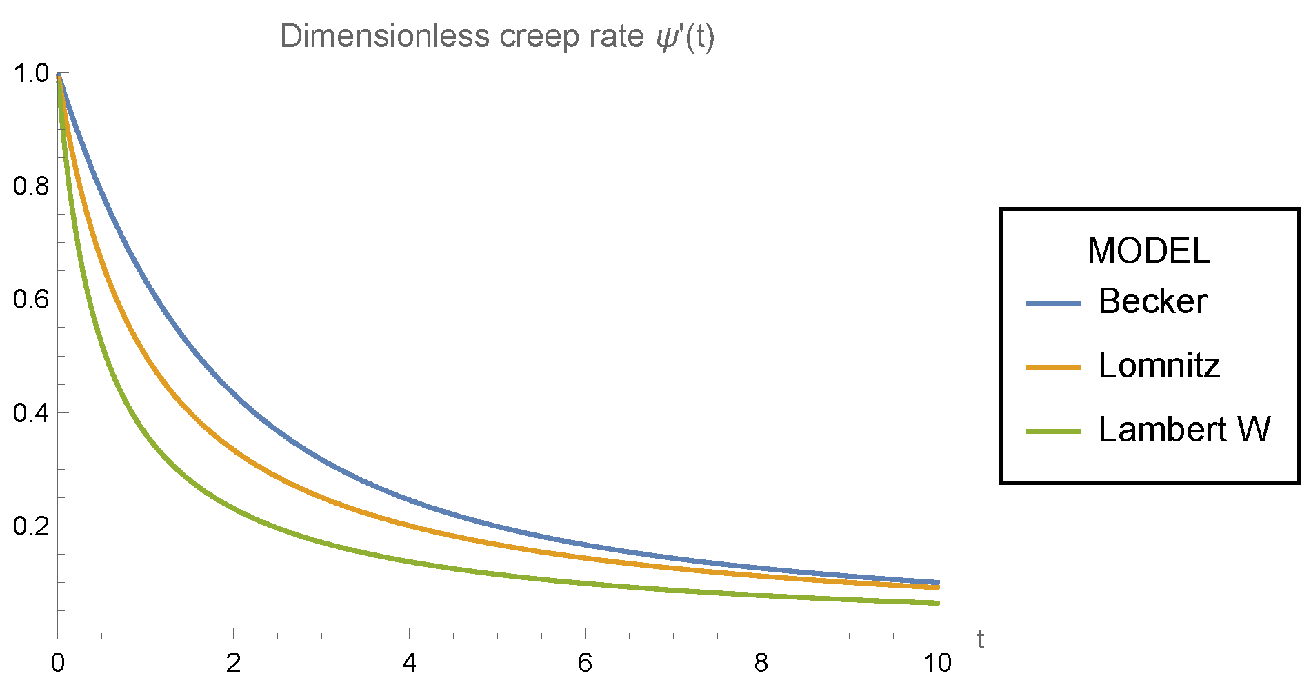
Figure 1 shows the dimensionless creep rate ${\psi }^{\prime }\left(t\right)$ for the Becker (15), Lomnitz (22), and Lambert (33) models. It is apparent that for $t\ge 0$, ${\psi }^{\prime }\left(t\right)$ is a monotonic decreasing function in all models, with ${\psi }^{\prime }\left(0\right)=1$. Also, Figure 1 suggests that ${\psi }_W^{\prime }\left(t\right)<{\psi }_L^{\prime }\left(t\right)<{\psi }_B^{\prime }\left(t\right)$ for $t>0$. The latter can be derived very easily by analytical methods, as it is shown in Appendix C.

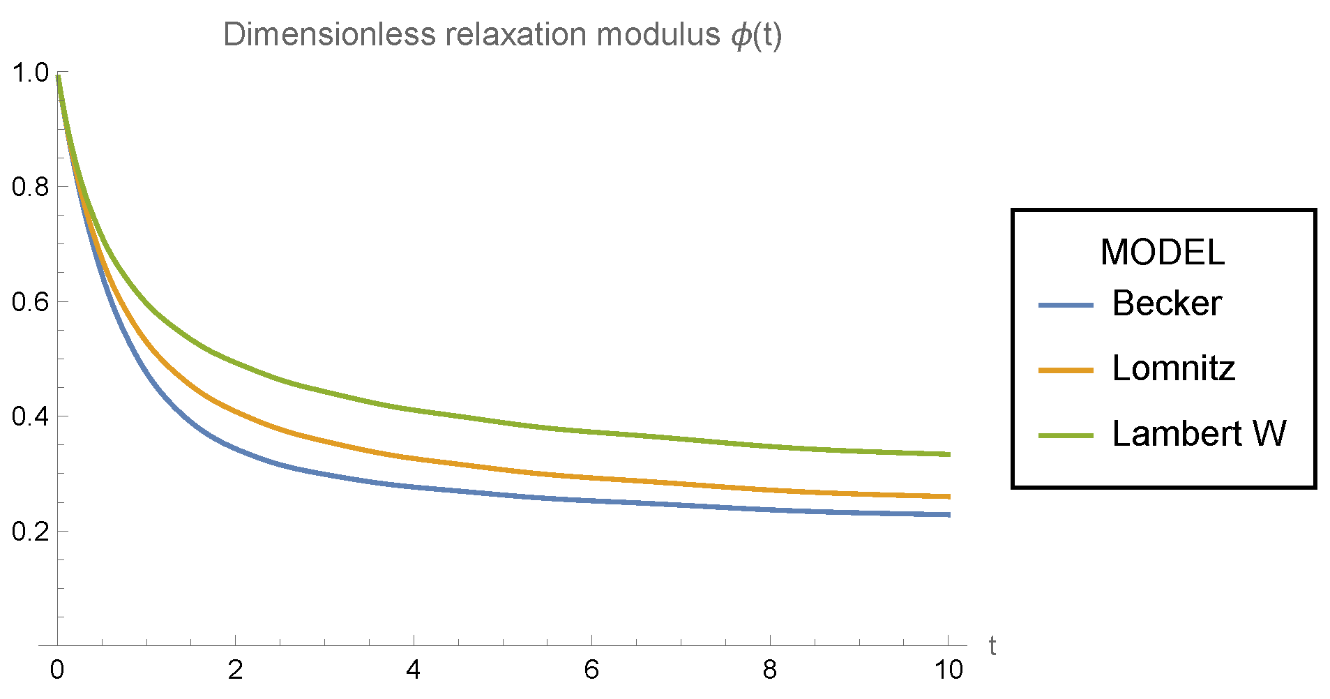
In Figure 2, the dimensionless relaxation modulus $\varphi \left(t\right)$ is plotted for all the models considered here. For this purpose, we have numerically evaluated (17), (24), and (34), computing the inverse Laplace transform with the Papoulis method [15] integrated into MATHEMATICA $13.2$. It is apparent that $\varphi \left(t\right)$ is a monotonic decreasing function for $t\ge 0$ with $\varphi \left(0\right)=1$ (9). Also, Figure 2 suggests that ${\varphi }_B\left(t\right)<{\varphi }_L\left(t\right)<{\varphi }_W\left(t\right)$ for $t>0$. Unlike the case of the creep rate, it does not seem that any analytical method derives the latter inequality.

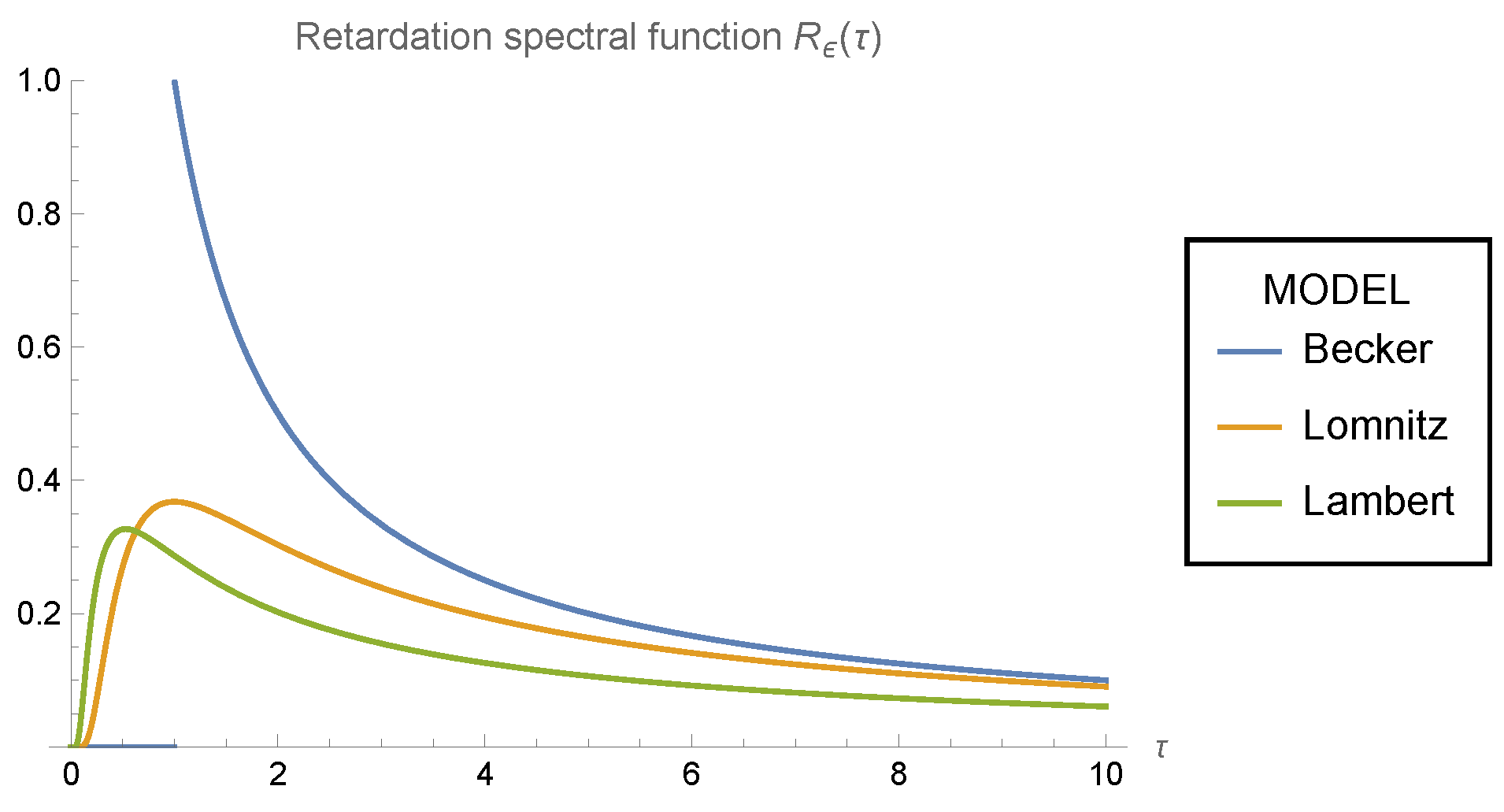
Figure 3 presents the retardation spectral function $R_{ϵ}\left(\tau \right)$ for the Becker (20), Lomnitz (29), and Lambert (37) models. It is worth noting that the graphs corresponding to the Lambert and Becker models verify the inequality derived in (40), i.e., $R_{ϵ}^W\left(\tau \right)<R_{ϵ}^B\left(\tau \right)$ for $\tau >1$.

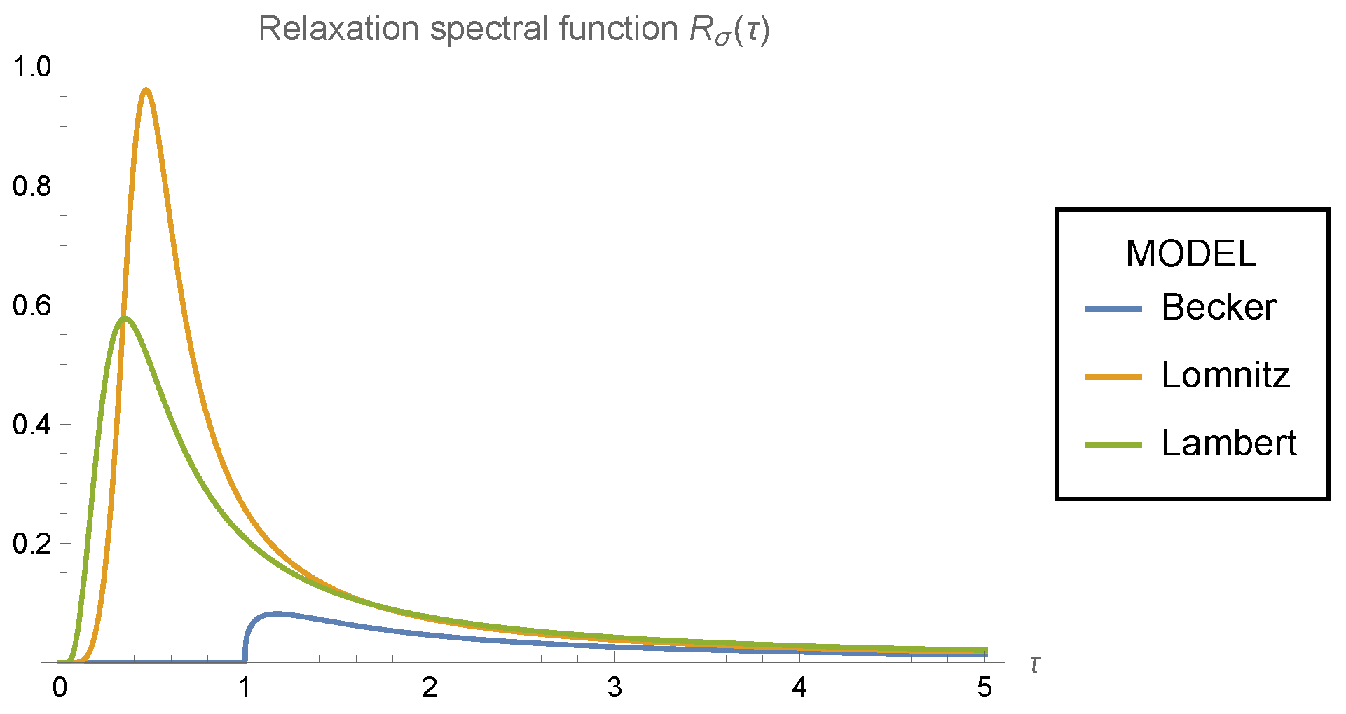
In Figure 4, the relaxation spectral function $R_{\sigma }\left(\tau \right)$ is plotted for the Becker (21), Lomnitz (30), and Lambert (41) models. Despite the fact that the plots for ${\psi }^{\prime }\left(t\right)$ and $\varphi \left(t\right)$ are quite similar for all the models, there is a great qualitative difference between the Becker model, and the Lomnitz and Lambert models with respect to the spectral functions $R_{ϵ}\left(\tau \right)$ and $R_{\sigma }\left(\tau \right)$, since the Becker model shows a discontinuity at $\tau =1$, but we have continuous functions for the other two models.

Finally, according to Figure 3 and Figure 4, it is apparent that the retardation $R_{ϵ}\left(\tau \right)$ and relaxation $R_{\sigma }\left(\tau \right)$ spectra for all the models considered here are non-negative functions, as aforementioned in the Introduction section. This is consistent with what was said above in (20) and (21) for the Becker model, (29) and (30) for the Lomnitz model, and (39) and (42) for the Lambert model.

7. Conclusions

We have compared some of the viscoelastic models for the law of creep reported in the literature, i.e., the Becker, Lomnitz, and Lambert models. For these models, we have computed in a much more efficient way the dimensionless relaxation modulus $\varphi \left(t\right)$ by numerically evaluating the inverse Laplace transform that appears in (10) instead of numerically solving the Volterra integral equation given in (8) (see ([2], Section 2.9.2)). The numerical inversion of the Laplace transform has been carried out by using the Papoulis method [15].

For the Becker and Lomnitz models, we have given novel closed-form formulas for the relaxation spectrum $R_{\sigma }\left(\tau \right)$, i.e., Equations (21) and (30). It is worth noting that these closed-form formulas allow us to compute $R_{\sigma }\left(\tau \right)$ in a much more efficient way than the numerical inversion of (2). As aforementioned in the Introduction section, the Becker and Lomnitz models have been considered in many physical applications; thus, these closed-form formulas are quite valuable in the field of viscoelastic materials.

Also, as a novelty, we have derived the retardation and relaxation spectra $R_{ϵ}\left(\tau \right)$ and $R_{\sigma }\left(\tau \right)$ in integral form for the Lambert model in (37) and (41). Again, these integral representations allow us to compute $R_{ϵ}\left(\tau \right)$ and $R_{\sigma }\left(\tau \right)$ very efficiently.

Further, we have proven that the spectral functions $R_{ϵ}\left(\tau \right)$ and $R_{\sigma }\left(\tau \right)$ are non-negative functions for all the models considered. It is worth noting as well that we have proven the interesting inequality $R_{ϵ}^W\left(\tau \right)<R_{ϵ}^B\left(\tau \right)$ for $\tau >0$ when comparing the retardation spectrum of the Lambert and Becker models.

In addition, we have compared all the models in terms of the behaviour of the dimensionless creep rate ${\psi }^{\prime }\left(t\right)$ in Figure 1, as well as the dimensionless relaxation modulus $\varphi \left(t\right)$ in Figure 2, and the spectral functions $R_{ϵ}\left(\tau \right)$ and $R_{\sigma }\left(\tau \right)$ in Figure 3 and Figure 4. From these graphs, we can appreciate that all the models are asymptotically equivalent, although not at the same rate. It is worth noting that the Becker model presents a discontinuity in the retardation spectral functions $R_{ϵ}\left(\tau \right)$ and $R_{\sigma }\left(\tau \right)$ at $\tau =1$, which is not present in the other models.

Finally, in Appendix C, we have proven the following inequality for the creep rate:

$${\psi }_W^{\prime }\left(t\right)<{\psi }_L^{\prime }\left(t\right)<{\psi }_B^{\prime }\left(t\right),t>0.$$

However, the following inequality for the dimensionless relaxation modulus:

$${\varphi }_B\left(t\right)<{\varphi }_L\left(t\right)<{\varphi }_W\left(t\right),t>0,$$

which is suggested in Figure 2, seems to be true, but we could not find any mathematical proof for it.