Explaining the Anomaly Detection in Additive Manufacturing via Boosting Models and Frequency Analysis

Abstract

Anomaly detection is an important feature in modern additive manufacturing (AM) systems to ensure quality of the produced components. Although this topic is well discussed in the literature, current methods rely on black-box approaches, limiting our understanding of why anomalies occur, making complex the root cause identification and the consequent decision support about the action to take to mitigate them. This work addresses these limitations by proposing a structured workflow designed to enhance the explainability of anomaly detection models. Using the wire arc additive manufacturing (WAAM) process as a case study, we examined 14 wall structures printed with INVAR36 alloy under varying process parameters, producing both defect-free and defective parts. These parts were classified based on surface appearance and welding camera images. We collected welding current and voltage data at a 5 kHz sampling rate and extracted features from both time and frequency domains using a knowledge-based approach. Isolation Forest, k-Nearest Neighbor, Artificial Neural Network, XGBoost, and LGBM models were trained on these features, and the results shown best performance of boosting models, achieving F1 scores of 0.927 and 0.945, respectively. These models presented higher performance compared to other models like k-Nearest Neighbor, whereas Isolation Forest and Artificial Neural Network posses lower performance due to overfitting, with an F1 score of 0.507 and 0.56, respectively. Then, by leveraging the feature importance capabilities of these models, we identified key signal characteristics that distinguish between normal and anomalous behavior, improving the explainability of the detection process and in general about the process physics.

1. Introduction

In the fourth industrial revolution, statistics is essential for transforming manufacturing, driving forward data-driven paradigms and innovations [1]. By leveraging data from sensors, machines, and production lines, manufacturers can uncover patterns and gain actionable insights. For instance, predictive maintenance can now forecast equipment failures before they happen, minimizing downtime and waste [2,3]. This impact has been amplified by the rise and the democratization of machine learning (ML), which, based in statistical principles, analyzes big data to enhance both offline and real-time quality inspection [4,5]. Today, ML can identify defects instantly from sensor data [6], further boosting efficiency and quality. Among the innovative fabrication processes revolutionizing the industry, additive manufacturing (AM) is emerging as the most widely used. Its appeal lies in its ability to enable rapid prototyping, offer high levels of product customization, and reduce material consumption [7]. Wire arc additive manufacturing (WAAM) has emerged as a cost-effective and sustainable alternative to traditional fabrication methods and other additive manufacturing techniques, particularly for producing medium to large-sized and complex metallic components [8,9,10]. The WAAM process, shown in Figure 1, is fundamentally an automated welding technique that require a precise optimization of parameters, procedure qualification, and monitoring, since it shares similar defects with the traditional welding methods it is based on, which are related on process parameters [11]. As with the other AM processes, a CAD model is used to obtain a path planning for a motion platform and a set of process parameters for the welding machine [12], which results in a final near-net shape part, which requires additional post-processing [13].

Currently, the number of research studies related to the application of ML in monitoring, optimization, and control of WAAM is exponentially increasing [14,15,16]. In particular, aiming to monitor the process and allow for the early identification of anomalies, several researchers proposed different techniques to develop online anomaly detection applications, employing different data sources and algorithms [17,18,19]. However, all the proposed methodologies are based on black-box approaches, since they rely on extracting statistical features from both time and frequency domain content of the time series data or automatic features from images [20,21,22,23], and they use these features as input to the ML algorithms. One issue with this approach, suggested by Norrish in [24], is that the WAAM systems might be treated as black-box machine tools, neglecting established welding quality control practices, further complicating the root cause identification and subsequent decision making. On the other hand, the high performance of these approaches should encourage researchers to explore methods that allow them to highlight how different features contribute to specific outcomes, such as defect generation. Understanding these contributions can offer valuable insights for decision-making modules, enabling them to take more informed actions [25,26,27]. Moreover, insights into how and why AI models make certain decisions are essential for enhancing their reliability, trustworthiness, and overall effectiveness in real-world applications. This recent growing demand for explainable AI models has led to increased interest in boosting models [28], primarily because of their ability to analyze feature importance and consequently improve the interpretability of results. Recent advancements have leveraged these models to identify and rank the importance of various features, helping researchers and practitioners understand how different factors contribute to the predictions of the models [29,30]. Despite the potential benefits of these methods for improving root cause identification, there is a noticeable absence of research in the literature on analyzing anomalies in additively manufactured parts.

In this research work, 14 wall structures using INVAR36 alloy were deposited with varying process parameters using the WAAM process. Both defect-free and defective parts were obtained from the conducted experimental campaign. During deposition, welding current and voltage data were collected, and features were extracted from both the time and frequency domains, following established methods in the field [19,31,32]. These features were used to train different boosting models, specifically XGBoost and LGBM, and other ML models for solving an online anomaly detection task. In this work, several contributions have been proposed. In particular, boosting models have been explored and the performance compared to other supervised and unsupervised learning to solve a classification problem in a small and unbalanced dataset scenario. Then, this work leverages the feature importance capabilities of boosting models to identify key signal characteristics that highlight the differences between normal and anomalous behavior of the process, enhancing the explainability of anomaly detection and allowing for more conscious decision making.

2. Materials and Methods

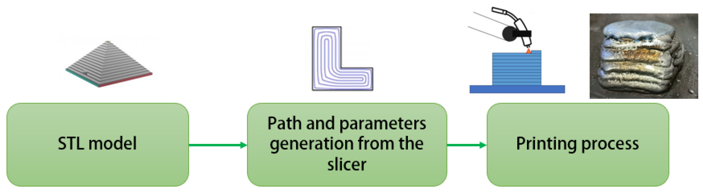
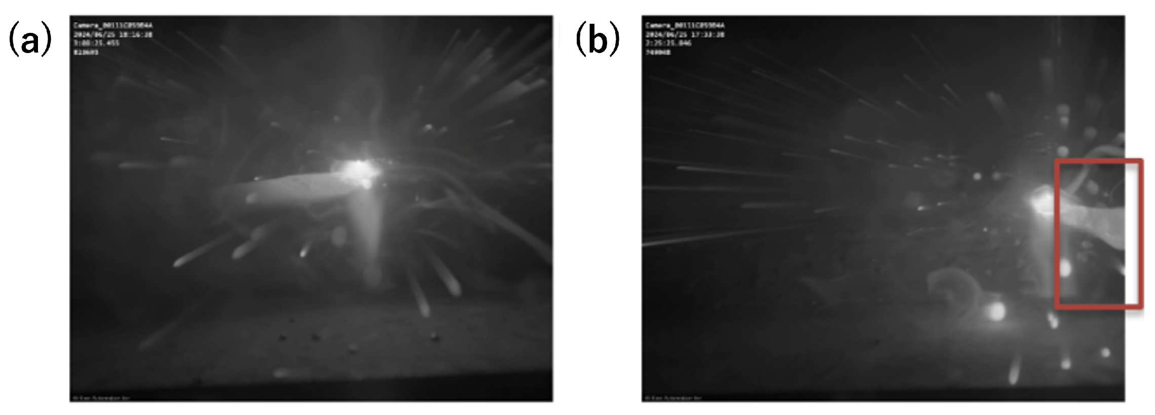
2.1. Experimental Setup

The experimental setup for this study, illustrated in Figure 2, is composed of an Omron Viper s850 robotic arm, a Miller Phoenix 456 power supply, and a multi-sensor acquisition system.

The material used is a 1.2 mm INVAR36 alloy wire, usually employed in the industry for its minimal dimensional changes under temperature variations. The mechanical proprieties and chemical composition are reported in

Table 1. Mechanical properties and chemical composition of Invar 36 (as welded).

Mechanical Properties	Value
Tensile strength [MPa]	>450
Elongation on 5d [%]	>25
Chemical Composition	Weight %
C	0.01
Mn	0.3
Si	0.12
S	0.004
P	<0.003
Ni	36
Ti	<0.003
Pb	0.001
Fe	63

.

The dataset used in this work was generated by printing 14 wall structures, each consisting of 10 layers, with all parameters kept constant during the deposition to ensure stability. The welding current and voltage were recorded at 5 kHz using a NI 6361 acquisition board and employed different process parameters for each wall, as outlined in

Table 2. Process parameters employed in this experimental campaign for printing INVAR36.

Wall No.	Wire Feed Speed [m/min]	Welding Voltage [V]	Welding Speed [mm/s]
1	3.5	19.0	6.5
2	4.0	19.0	9.0
3	3.5	22.5	4.0
4	3.5	21.0	8.0
5	3.5	19.0	9.0
6	3.5	20.0	4.0
7	3.0	19.0	6.5
8	2.0	20.0	6.5
9	6.0	19.0	9.0
10	6.0	21.0	9.0
11	4.0	22.5	6.5
12	3.0	22.5	9.0
13	4.0	19.0	8.0
14	3.0	20.0	9.0

. The gas flow rate and the contact to workpiece distance (CTWD) were fixed to 18 L/min and 15 mm, respectively. Additionally, a welding camera (Xiris XCV-1000) was employed to capture images of the process, which were subsequently used to label the collected data (see Figure 3). In fact, due to parameter selection, several defects occurred along the deposited layer, such as layer collapse or porosity. Aiming to develop a real-time anomaly detection module, data were processed by extracting 1 s windows from each deposited layer, as illustrated in Figure 4, and a label of anomaly is assigned if a defect occurred during the 1 s deposition using the video recorded with the welding camera.

In this work, once features have been extracted from the 1 s length signals, they are used as input to the machine learning (ML) algorithm, as shown in the workflow in Figure 5. This allows the proposed methodology to be utilized online, since a buffer of 5000 samples can be filled and then processed first with feature extraction and subsequently directly with ML.

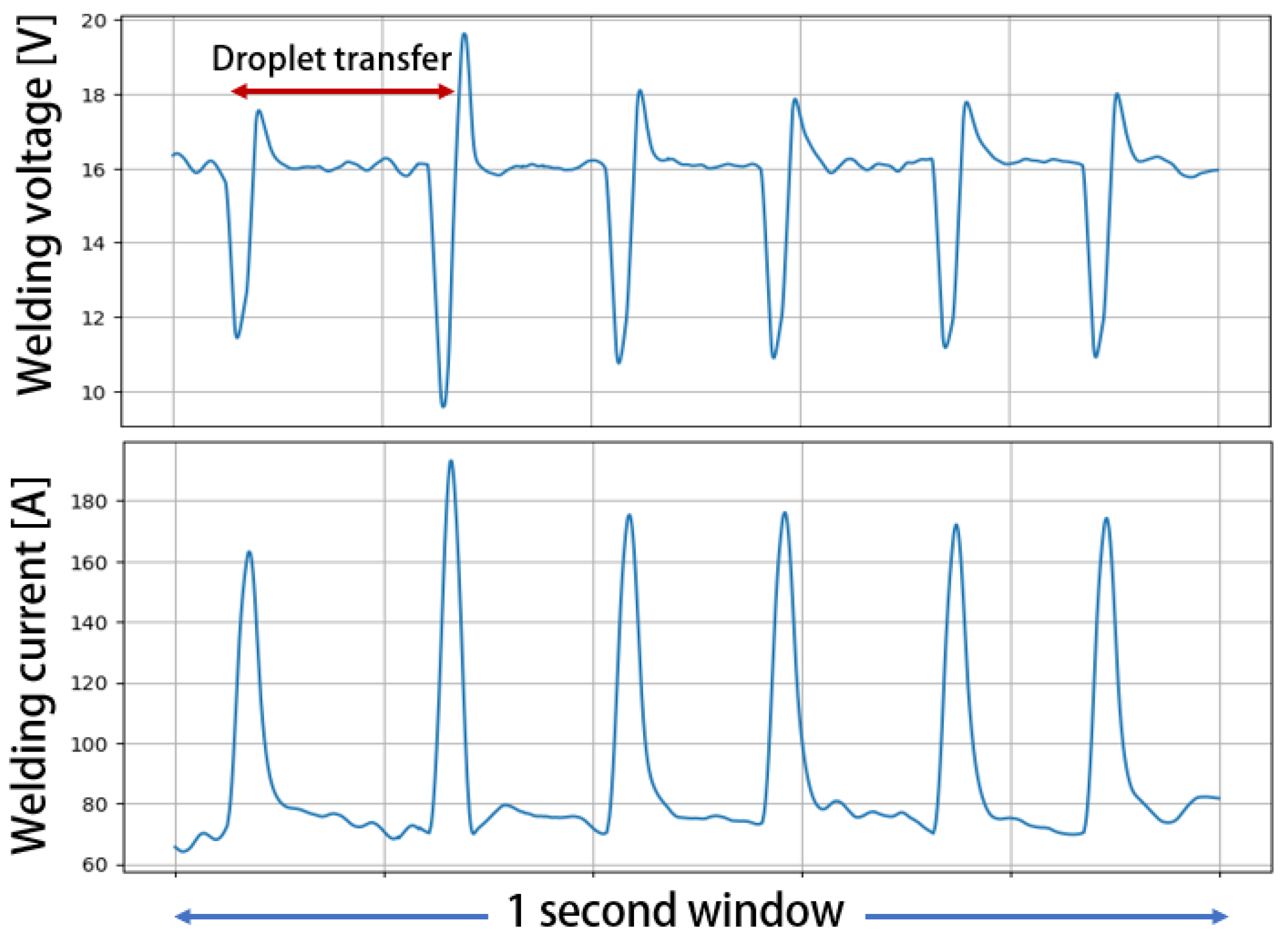
2.2. Data Preprocessing and Features Extraction

The dataset obtained as described above consist of 1698 samples, which result into an unbalanced dataset, with 344 anomalies with a label equal to 1 and 1354 normal cases, with a label equal to 0. In the proposed framework, knowledge-based features were extracted. Several studies have demonstrated the importance of the frequency information content of the welding current and welding voltage signals to asses the quality of the deposition [33]. Therefore, in this work, frequency domain features have been extracted using both fast Fourier transform (FFT) and discrete wavelet transform (DWT). Specifically, features such as energy, variance, median, skewness, and kurtosis were extracted from an 7-level decomposition using discrete wavelet transform (DWT) and from the FFT magnitude spectrum for each sample. Furthermore, the same features were extracted from the raw signals of welding current and welding voltage for a total of additional 10 features that describe the system behavior in the time domain [34,35]. Each sample consists of a 1 s welding process with current and voltage signals, resulting in a total of 100 features per sample.

When using current and voltage sensors for signal data collection, there are no significant challenges in terms of data acquisition, as most commercially available data acquisition systems (DAQs) are capable of capturing data at frequencies up to 5 kHz [36]. This study employed a suitable DAQ device that supports this data acquisition rate. However, one of the primary challenges arises during the preprocessing phase related to the selection of an appropriate window size for real-time monitoring. If the window size is too large, the frequency domain analysis for feature extraction may take longer, and the extracted features could become more global, complicating the localization of anomalies. Conversely, if the window size is too small, it may not capture enough data to derive meaningful features from the signal [37]. Given that windowing approaches for real-time signal monitoring are not yet extensively explored in the literature, we opted for a 1 s window based on prior studies that demonstrated its effectiveness. This choice strikes a balance between computational efficiency and the ability to extract relevant features for anomaly detection.

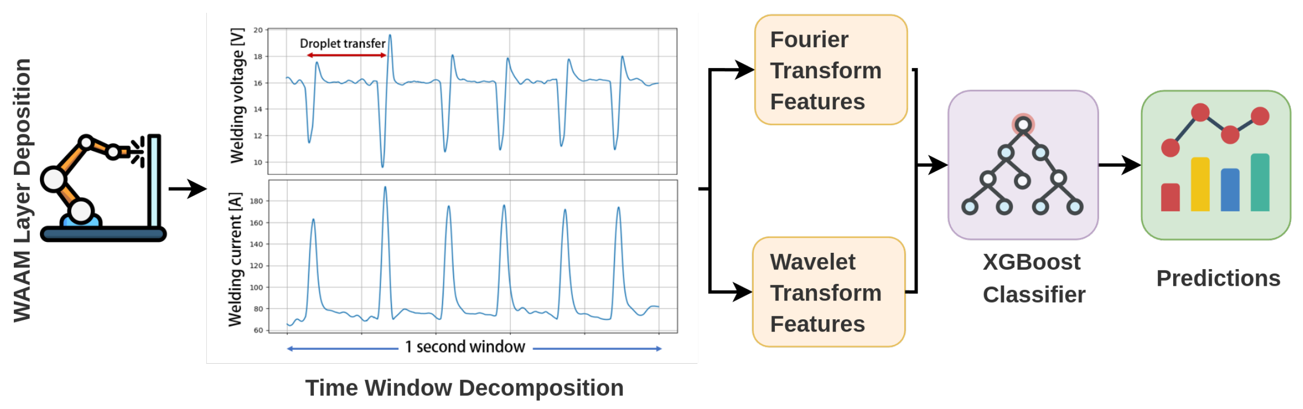
2.2.1. Fast Fourier Transform Features

The Fourier transform offers a frequency-domain representation of a signal by decomposing it into a sum of sinusoidal components, each with different amplitudes and frequencies. This method effectively reveals the frequency content of a signal. However, it lacks temporal resolution, making it less suitable for signals where the frequency response changes significantly within a given time window. This limitation is particularly relevant for welding signals, such as those from the natural dip transfer process, where frequency variations occur over short time intervals. Mathematically, the Fourier transform of a continuous signal $x\left(t\right)$ is defined by Equation (1).

$$X\left(f\right)={\int }_{-\infty }^{\infty }x\left(t\right)e^{-j2\pi ft}dt$$

(1)

where $X\left(f\right)$ represents the frequency-domain representation of the signal $x\left(t\right)$. The discrete Fourier transform (DFT) is used for discrete signals and is given by Equation (2). In this formulation, $X\left[k\right]$ provides the frequency components of the discrete signal $x\left[n\right]$, where N is the number of samples. The fast Fourier transform (FFT) is an efficient algorithm to compute the DFT.

$$X\left[k\right]=\sum _{n=0}^{N-1}x\left[n\right]e^{-j2\pi kn/N}$$

(2)

The main advantage of the Fourier transform is its ability to decompose a signal into its constituent frequencies. This makes it particularly useful for analyzing signals with periodic components or for tasks such as filtering and spectral analysis. However, the Fourier transform has limitations, particularly in capturing time-varying features of a signal, as it provides a global frequency representation without time localization.

In this work, the FFT of current and voltage signals was performed after subtracting the mean from a 1 s window. Following this, FFT was computed for the centered vectors of both current and voltage signals, and statistical features such as energy, skewness, kurtosis, and variance were extracted, resulting in a total of 10 features. An example of the FFT response for normal behavior data is illustrated in Figure 6. Although these features provide a global overview of the frequency characteristics of the data and can be used directly in machine learning algorithms, they do not capture local variations. To address this, a DWT is applied to uncover localized features within the frequency domain.

2.2.2. Discrete Wavelet Transform Features

The discrete wavelet transform (DWT) provides a time–frequency representation of a signal, offering an advantage over the Fourier transform, which only captures frequency information. In fact, unlike the Fourier transform, which uses sinusoids as basis functions, the DWT uses wavelets—localized waveforms that vary in both time and frequency. This allows the DWT to capture both high-frequency details and low-frequency trends [38].

Mathematically, the DWT decomposes a discrete signal $x\left[n\right]$ into different levels, each containing a low-frequency (approximation) and a high-frequency (detail) component using scaling functions ${\varphi }_{j,k}\left(x\right)$ and wavelet functions ${\psi }_{j,k}\left(x\right)$. The multi-resolution nature of the DWT makes it particularly useful in applications like image compression [39], noise reduction [40], and feature extraction from non-stationary signals, as in the case of welding signals [41,42].

If the wavelet functions ${\psi }_{j,k}\left(x\right)$ and the scaling functions ${\varphi }_{j,k}\left(x\right)$ form an orthogonal basis, then the signal $f\left(x\right)$ can be expressed as a sum of its approximation and detail components, as in Equation (3), where the approximation $f_n\left(x\right)$ is given by Equation (4) and the detail $f_n^{\perp }\left(x\right)$ is represented as in Equation (5).

$$f\left(x\right)=f_n\left(x\right)+f_n^{\perp }\left(x\right)$$

(3)

$$f_n\left(x\right)=\sum _{k=-\infty }^{\infty }{a}_{n,k}{2}^{n/2}\varphi (2^{n}x-k)$$

(4)

$$f_n^{\perp }\left(x\right)=\sum _{j=n}^{\infty }\sum _{k=-\infty }^{\infty }{b}_{j,k}{2}^{j/2}\psi (2^{j}x-k)$$

(5)

In this formulation, the coefficients $a_{n,k}$ and $b_{j,k}$ are the approximation and detail coefficients, with the functions ${\varphi }_{n,k}\left(x\right)=2^{n/2}\varphi (2^{n}x-k)$ and ${\psi }_{j,k}\left(x\right)=2^{j/2}\psi (2^{j}x-k)$ representing the scaled and translated versions of the scaling function $\varphi \left(x\right)$ and the wavelet function $\psi \left(x\right)$. The choice of wavelet functions $\psi \left(x\right)$ and scaling functions $\varphi \left(x\right)$ depends on the particular family of wavelets used, as different families provide different characteristics suited for specific applications:

• The Haar wavelet, known for its simplicity, is the most basic wavelet. Its scaling function is a step function, making it easy to compute and suitable for certain applications, particularly those requiring piecewise constant approximations. However, a notable drawback of the Haar wavelet is its lack of translational invariance. This means that a small shift in the signal can result in a significantly different wavelet decomposition. In practical terms, this can lead to instability or inconsistent results when analyzing signals that do not align perfectly with the wavelet’s step-like structure. As a result, Haar wavelets may not perform well in applications like complex waveform welding processes.
• Daubechies wavelets are a popular family of wavelets distinguished by their compact support and the ability to efficiently capture both time and frequency information. Their effectiveness increases with the order of the wavelet, allowing them to handle signals with sharp transitions or high-frequency components due to their vanishing moments, which facilitate precise signal approximation. Despite these advantages, Daubechies wavelets have a lack of symmetry, which can make them less suitable for tasks such as image reconstruction or certain filtering applications where symmetry is beneficial. Nevertheless, Daubechies wavelets are extensively used in welding applications, where their properties are particularly well-suited for analyzing and processing signals related to welding processes [43,44].
• Coiflets wavelets are designed to enhance symmetry and vanishing moments, improving signal approximation compared to other wavelets. However, the increased computational complexity associated with Coiflets may not always be justified, especially when compared to Daubechies wavelets. Coiflets are particularly beneficial when Daubechies wavelets struggle with symmetry, as Coiflets provide better phase alignment and feature reconstruction. Therefore, Coiflets are a preferable choice in scenarios where symmetry is crucial and Daubechies wavelets’ performance is insufficient due to their asymmetry.

Once the detail coefficients are extracted from the signal, they represent frequencies in the ranges $[f/(2·i),f/(2·i+1)$, where i ranges from 1 to the number of levels L. The final approximation captures frequencies in the range $[0,f/(2·L\left)\right)$, with L denoting the number of levels and f representing the Nyquist frequency of the sampling rate. From this decomposition, various statistical measures such as mean, variance, kurtosis, skewness, and median can be computed, analogous to the analysis performed with FFT spectra. This results in $5\times (L+1)$ features, which collectively represent the complex time–frequency content of the signal.

In welding tasks, selecting the appropriate number of decomposition levels is a complex decision that depends on the frequency response of the signal. For example, in this work, the short-circuit nature of the deposition means that most of the frequency response is concentrated within a lower frequency bandwidth. To effectively separate these frequencies, several decomposition levels are required due to the high sampling rate used. In the context of this work, with the sample frequency of 5 kHz, the value of Nyquist frequency is $f=2500$. A 7-level decomposition was performed using a Daubechies wavelet of 4 order. This decomposition resulted in levels similar to those illustrated in Figure 7. From these decompositions, 40 features were extracted for each sensor. Combined with the 5 features obtained from the FFT analysis, a total of 45 features for sensor were derived for a total of 90 features for sample. These features describe each second of deposition and its frequency content, which can subsequently be classified using various machine learning algorithms.

2.3. Boosting Models

Boosting is a powerful ensemble technique in machine learning that combines the predictions of several base estimators to improve overall model performance. Unlike traditional methods, boosting algorithms sequentially train weak learners, typically decision trees, with each new model attempting to correct the errors made by the previous ones. This iterative approach reduces bias and variance, leading to highly accurate predictive models. Among the popular boosting algorithms, XGBoost (extreme gradient boosting) and LightGBM (light gradient boosting machine) are widely used due to their robustness and efficiency.

XGBoost is noted for its advanced boosting implementation that constructs a strong predictor by combining numerous weak predictors. Each successive tree in XGBoost focuses on correcting the residuals of the previous tree, thereby progressively enhancing the model’s accuracy. The objective function in XGBoost incorporates a regularization term to prevent overfitting and is defined as

$$\mathcal{L}\left(t\right)=\sum _{i=1}^{n}l(y_i,{\hat{y}}_i^{(t-1)}+f_t\left(x_i\right))+\sum _{k=1}^t\Omega \left(f_k\right)$$

(6)

where l represents a generic loss function, ${\hat{y}}_i^{(t-1)}$ is the prediction at iteration $t-1$, $f_t$ is the new tree added at iteration t, and $\Omega \left(f_k\right)$ is the regularization term for the kth tree. The regularization function $\Omega \left(f\right)$ for an individual tree is typically defined as

$$\Omega \left(f\right)=\gamma T+{\displaystyle \frac{1}{2}}\lambda \sum _{j=1}^T{w}_j^2$$

(7)

where T denotes the number of leaves in the tree and $w_j$ are the weights of the leaves. XGBoost is particularly known for its scalability and performance in both regression and classification tasks. However, its complexity and the necessity for careful tuning of hyperparameters can be seen as drawbacks.

LightGBM, on the other hand, is recognized for its efficiency and optimized implementation of boosting. Each new tree in LightGBM aims to correct the residual errors of the previous one, continually improving the model’s performance. Similar to XGBoost, the objective function in LightGBM includes a regularization term and the equations behind it are the same as written in (6) and (7).

LightGBM is designed to be highly efficient and scalable, using histogram-based algorithms to find the best splits, which significantly reduces the training time compared to traditional gradient boosting algorithms. Additionally, LightGBM supports parallel and GPU learning, making it suitable for large-scale datasets. Its main drawback is that it can be sensitive to parameter tuning and may require extensive experimentation to achieve optimal performance.

In the context of classification, both XGBoost and LightGBM can handle binary and multi-class classification tasks. For binary classification, the loss function $l(y,\hat{y})$ is typically the logistic loss:

$$l(y,\hat{y})=-[ylog\left(\sigma \left(\hat{y}\right)\right)+(1-y)log(1-\sigma \left(\hat{y}\right))]$$

(8)

where $\sigma \left(\hat{y}\right)$ is the sigmoid function, defined as $\sigma \left(\hat{y}\right)={\displaystyle \frac{1}{1+e^{-\hat{y}}}}$. This function maps the raw prediction scores to probabilities, allowing for the classification of instances into two classes.

For multi-class classification, both models use the softmax loss function. The softmax function is defined as

$$\sigma \left({\hat{y}}_i\right)={\displaystyle \frac{e^{{\hat{y}}_i}}{{\sum }_{j=1}^K{e}^{{\hat{y}}_j}}}$$

(9)

where K is the number of classes, and ${\hat{y}}_i$ is the raw score for the ith class. The corresponding loss function is the categorical cross-entropy loss:

$$l(y,\hat{y})=-\sum _{k=1}^K{y}_{k}log\left(\sigma \left({\hat{y}}_k\right)\right)$$

(10)

where $y_k$ is a binary indicator (0 or 1) if class label k is the correct classification for the given observation.

2.4. Metrics for Performance Evaluation

To evaluate the performance of a classification model, several metrics are commonly used, including precision, recall, the F1-score, and the precision–recall curve, particularly when handling imbalanced datasets. Precision is defined as the ratio of true positives (TP) to the sum of true positives and false positives (FP), measuring the accuracy of the positive predictions made by the model. Mathematically, this is expressed as

$$\mathrm{Precision}={\displaystyle \frac{\mathrm{TP}}{\mathrm{TP}+\mathrm{FP}}}$$

(11)

Recall, also known as sensitivity or the true positive rate, quantifies the model’s ability to correctly identify all positive instances. It is the ratio of true positives to the sum of true positives and false negatives (FN), given by

$$\mathrm{Recall}={\displaystyle \frac{\mathrm{TP}}{\mathrm{TP}+\mathrm{FN}}}$$

(12)

The F1-score is the harmonic mean of precision and recall, providing a single measure that balances the trade-off between these two metrics. It is particularly useful in situations with imbalanced class distributions. The F1-score is defined as

$$\mathrm{F}1\text{-}\mathrm{score}=2\times {\displaystyle \frac{\mathrm{Precision}\times \mathrm{Recall}}{\mathrm{Precision}+\mathrm{Recall}}}$$

(13)

Another interesting metric for the evaluation of classification is the Matthews correlation coefficient (MCC), often preferred over the F1 score, especially in situations with imbalanced classes, because it provides a more comprehensive evaluation of the entire confusion matrix. Although the F1 score focuses primarily on the balance between precision and recall, it does not account for true negatives, which can be crucial in scenarios where one class significantly outnumbers the other. The MCC takes into consideration all four confusion matrix categories (true positives, true negatives, false positives, and false negatives), making it a better metric for assessing model quality in such cases:

$$MCC={\displaystyle \frac{\mathrm{TP}·\mathrm{TN}-\mathrm{FP}·\mathrm{FN}}{\sqrt{(\mathrm{TP}+\mathrm{FP})(\mathrm{TP}+\mathrm{FN})(\mathrm{TN}+\mathrm{FP})(\mathrm{TN}+\mathrm{FN})}}}$$

(14)

In addition to these scalar metrics, the precision–recall (PR) curve is a graphical tool that visualizes the trade-off between precision and recall across different classification thresholds. The precision–recall area under the curve (PR AUC) provides an aggregate measure of the model’s performance, where a higher area indicates better performance, particularly in cases where the positive class is rare. The PR curve is often preferred over the receiver operating characteristic (ROC) curve in these scenarios as it provides a more focused analysis of the positive class performance [45]. By using these metrics, we can obtain a comprehensive evaluation of the classification model’s ability to handle various class distributions and make accurate predictions. F-score and PR-AUC are particularly valuable metrics for addressing anomaly detection problems, especially when supervised learning is applied to unbalanced datasets. In industrial processes, like the one proposed in this study, this poses a significant challenge, as imbalanced data often lead to overfitting, producing unreliable results. This issue is difficult to avoid, as introducing anomaly data is often costly, and, in many cases, anomalies must be artificially induced in the system, which is typically impractical. However, this does not mean supervised approaches are unviable. In fact, users can still leverage the benefits of high generalization and performance compared to their unsupervised counterparts to develop anomaly detection tasks, but relying solely on accuracy to evaluate performance in such cases can be inaccurate. Instead, metrics like the F-score, which balance precision and recall, are more suitable for assessing the model’s ability to detect anomalies. These metrics provide a clearer picture of the model’s generalization capacity and its potential for overfitting on the test dataset.

3. Results

3.1. Recap of the Proposed Methodology

In this study, various process parameters were utilized to deposit 14 walls using a wire arc additive manufacturing (WAAM) process, each consisting of 10 layers. Data, including welding current and voltage, were collected at a sampling rate of 5 kHz, as these signals are strongly linked to arc stability and the occurrence of defects in the AM parts. To develop an online anomaly detection algorithm, the signals were divided into 1 s windows, with each window classified based on arc sound, welding camera images, and the surface appearance of the deposited layer (e.g., detecting defects such as humping, arc instability, excessive spatter, porosity, etc.). Features in both the time and frequency domains were extracted to capture both global system behavior and localized information across different frequency bands. The results were then compared across various machine learning classifiers, including k-Nearest Neighbors, Isolation Forest, and advanced classifiers like XGBoost, LightGBM and neural networks.

3.2. Model Hyperparameters

The hyperparameters for the proposed models were manually tuned, and only the best results are reported in the discussion section. For the k-Nearest Neighbors (kNN) algorithm, a value of $K=33$ was selected, with the distance between data points computed using the Euclidean distance metric.

In the case of the Isolation Forest, the model was configured with 100 trees, each trained on 256 randomly selected samples, and a contamination value of 0.1 was applied, representing the expected proportion of anomalies in the dataset.

For the neural network model, we propose an advanced state-of-the-art architecture consisting of two hidden layers, each with 64 neurons and a ReLU activation function. This configuration is chosen to effectively capture complex patterns in the data. For the training process, we utilized a cross-entropy loss function, which is well-suited for classification tasks.

For the XGBoost model, a maximum tree depth of six was chosen, combined with a learning rate of 0.3 and 100 estimators (trees), with no regularization applied. Similarly, the LightGBM model was tuned with a learning rate of 0.1, using 100 trees and 31 leaves per tree, also without any regularization.

All the algorithms were trained on 85% of the data while the test set is obtained with the reaming 15%, for a total of 254 samples that contain both normal and anomaly data.

3.3. Discussion of the Results

The comparison of various models is summarized in

Table 3. Performance metrics for LightGBM, XGB, ANN, kNN, and Isolation Forest models.

Model	Recall	Precision	F1-Score	MCC
Light Gradient-Boosting Machine (LightGBM)	0.929	0.963	0.945	0.931
eXtreme Gradient-Boosting (XGB)	0.911	0.911	0.927	0.908
K-Neighbors Classifier	0.875	0.875	0.916	0.895
Isolation Forest	0.339	0.339	0.507	0.504
Neural Network	0.5	0.63	0.56	0.52

, which reports their recall, precision, F1-score, and MCC.

Among the models evaluated, LightGBM demonstrates the highest performance across all metrics. It achieves a precision of 0.929, a recall of 0.963, and an F1-score of 0.945. These results indicate that LightGBM is exceptionally effective at detecting anomalies. The high recall reflects its ability to identify a large proportion of actual anomalies, whereas the high precision shows that the model correctly classifies anomalies most of the time. Moreover, XGBoost shows competitive performance, though slightly lower than LightGBM, with a precision and recall both at 0.911, and an F1-score of 0.927. The k-Nearest Neighbors (kNN) algorithm performs worse than both boosting models, with a precision and recall of 0.875 and an F1-score of 0.916. The lower precision indicates that kNN is more prone to false positives, meaning it misclassifies more normal instances as anomalies. Although the F1-score is still good, the performance is lower than for the LightGBM and XGBoost models, suggesting that kNN may not be as well-suited for this particular task. Finally, Isolation Forest exhibits significantly weaker performance, with a precision and recall of only 0.339 and an F1-score of 0.507. This indicates that Isolation Forest struggles to correctly identify anomalies in this dataset, with a high rate of false positives (low precision) and an inability to capture most of the true anomalies (low recall). Although Isolation Forest comes from the same family of classifier of XGBoost and LightGBM, it is more prone to overfit, leading to worse accuracy on the test dataset. Finally, issues related to overfitting impact the ability of the neural network to make accurate predictions, resulting in a final F1-score of 0.56, which performs slightly better than the Isolation Forest in this case. The comparison of results highlights that boosting models perform better in scenarios with small and unbalanced datasets, and that the development of more complex models should be carefully considered, as it may not be worthwhile.

To gain a deeper understanding of the differences between LightGBM and XGBoost, Figure 8 presents the precision–recall area under the curve (PR-AUC) and the confusion matrix for both models. LightGBM effectively reduces the number of false alarms, decreasing them from three to two, while also minimizing missed real anomalies, reducing them from five to two.

3.4. Explainability of the Model

Explainability is crucial for understanding how machine learning models make predictions. Beyond enhancing trust in the models, explainability also provides insights into the underlying complexities of the processes being modeled. This understanding can reveal additional information beyond the classification labels, offering a deeper comprehension of the phenomena involved. In the proposed boosting models, explainability is achieved through feature importance metrics, which evaluate each feature’s impact on model performance by measuring its contribution to reducing impurity. Additionally, SHAP values could be used to offer more granular insights, providing detailed, instance-level explanations of feature contributions. The results of features importance of the best model, namely LightGBM, are shown in Figure 9 for the most relevant features, selected with a importance score greater then 100. The analysis reveals that the LightGBM importance scores identify several key features: the skewness of the voltage time series, the variance of the current time series, the energy of the FFT spectrum for current, and the variance of the response of both welding current and welding voltage within the 0–357 Hz bandwidth.

Skewness measures the asymmetry of a data distribution around its mean. In industrial processes, deviations from the normal distribution may indicate potential issues or anomalies. A high skewness in the voltage time series suggests that the heat input supplied to the material is uneven, which could indicate process instability or irregularities.

On the other hand, variance quantifies how much values in the time series deviate from the mean. High variance in the welding current signal indicates an unstable deposition process. Since the dip transfer process primarily occurs in the 0–357 Hz frequency bandwidth, the variance in this bandwidth reflects process instabilities.

Finally, the energy of the FFT response directly indicates the power and heat input supplied to the material. Therefore, all these features—skewness, variance, and FFT energy—are related to the consistency of heat input during deposition. Although some variance is normal in dip transfer processes, excessively high values can signal instability, lack of fusion, or porosity.

3.5. Future Developments

In developing an anomaly detection software module, the use of explainable AI models, like the presented boosting algorithms, is essential for understanding the mechanisms behind specific predictions. By examining feature importance, the system can pinpoint the variables most strongly linked to anomalies or deviations from expected behavior. Once these key features are identified, they can be further analyzed to uncover patterns and trends associated with anomalies, such as lack of fusion in welding or the presence of porosity.

To achieve this, the training dataset can be clustered based on the values of these important features, allowing the system to segment the data into distinct categories. These clusters can highlight different types of anomalies, each potentially requiring different responses or actions. This data segmentation also enables human operators or automated systems to interpret anomalies more effectively, leading to informed decisions.

This approach paves the way for future developments in predictive maintenance, quality control, and decision making. In predictive maintenance, for instance, understanding which sensor readings or operational metrics contribute to machine failures can enable more targeted and timely interventions. In quality control, identifying key factors that lead to defective products allows for more proactive corrective measures, such as improving the wire feed speed or reducing the welding speed if an instability or an humping defect is detected.

Although the proposed approach offers potential benefits, it represents a target for future enhancements in this work, particularly for industrial applications. Future developments could aim to improve the model’s explainability by incorporating human-readable visualizations and providing more detailed analyses of feature importance.

4. Conclusions

This study explores new methodologies to enhance the explainability of anomaly detection in additive manufacturing. Specifically, it focuses on the wire arc additive manufacturing (WAAM) process, where 14 wall structures were printed using INVAR36 alloy under different process parameters, resulting in both defect-free and defective parts, which were classified based on surface appearance and images captured by a welding camera. During the experimental campaign, welding current and voltage data were collected at a sampling rate of 5 kHz, and the extracted features from both the time and frequency domains have were used as input to different ML models, namely XGBoost, LightGBM, Isolation Forest, k-Neighbors and Artificial Neural Network (ANN) classifiers. The results demonstrated that the XGBoost and LGBM models achieved high performance, with F1 scores of 0.927 and 0.945, respectively, indicating their effectiveness in handling unbalanced datasets without a loss in performance. In comparison, k-Nearest Neighbors achieved an F1 score of 0.916, while the unsupervised Isolation Forest reached an F1 score of 0.507, underscoring the strength of boosting algorithms for this task. Finally, ANNs performed poorly, achieving an F1-score of 0.56, primarily due to overfitting caused by the small and unbalanced nature of the collected dataset. Additionally, by leveraging the ability of the boosting models to identify feature importance, it is possible to identify the key signal characteristics that distinguish between normal and anomalous behavior, thereby improving the explainability of the anomaly detection process. Specifically, for the INVAR36 alloy wire employed and the process parameters used, the variance of the frequency response within the 0–357 Hz range for both welding current and voltage, and the mean energy of the FFT spectrum of the voltage, were found to be the most important features. Notably, variance and skewness helped detect outliers due to asymmetry in the response and narrowing in amplitude at this frequency bandwidth, in which the physical phenomena of the droplet transfer happen. The key contributions of this work are summarized and listed below:

• We compared performance in online anomaly detection of different ML models once a small and unbalanced dataset is available.
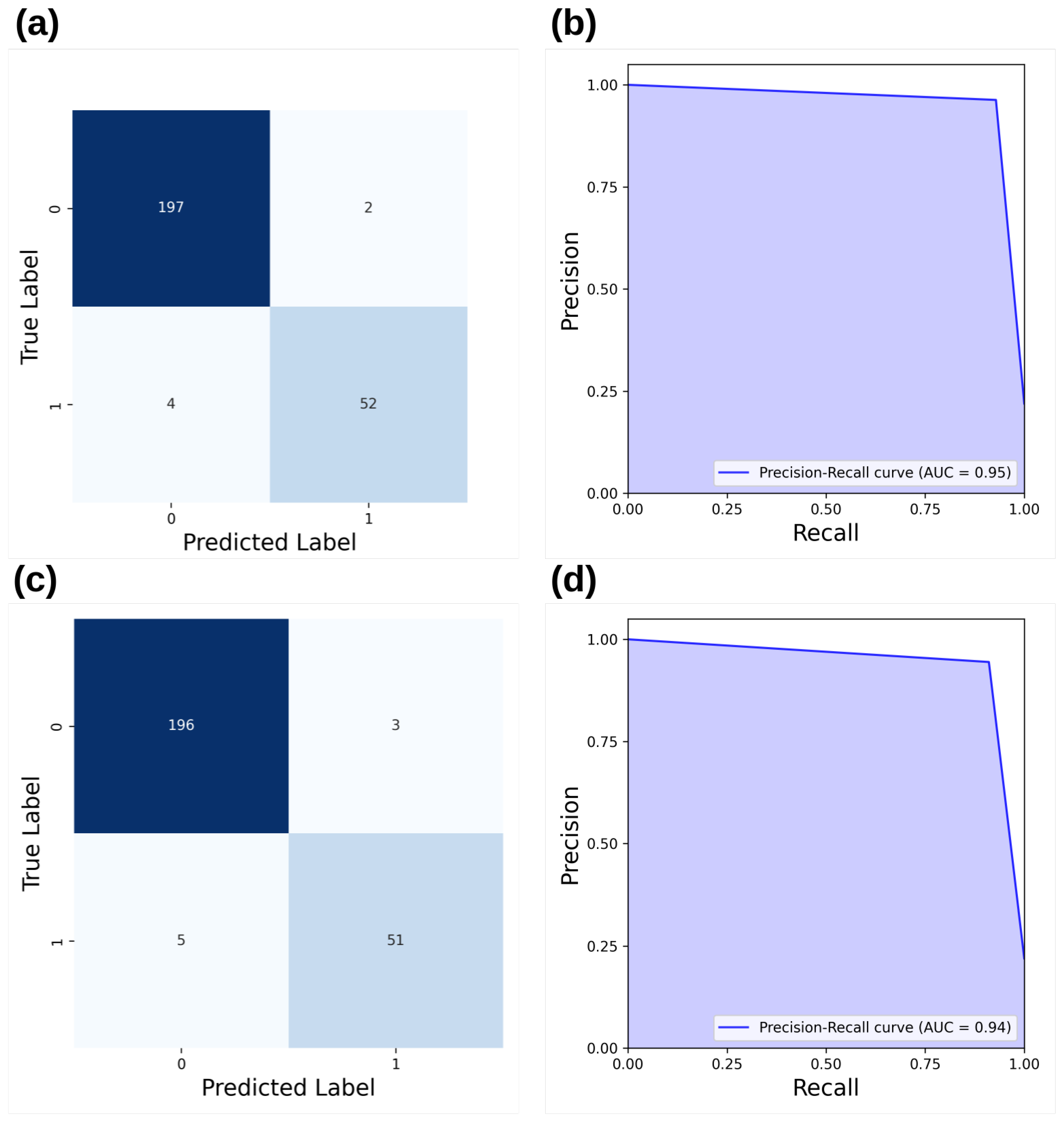
• The results showed high performance from XGBoost (F1 score: 0.927) and LGBM (F1 score: 0.945), proving their effectiveness on small and unbalanced datasets. The k-Nearest Neighbors method achieved 0.916, while Isolation Forest and ANN scored 0.507 and 0.56, respectively, highlighting the superiority of boosting methods in this scenario.
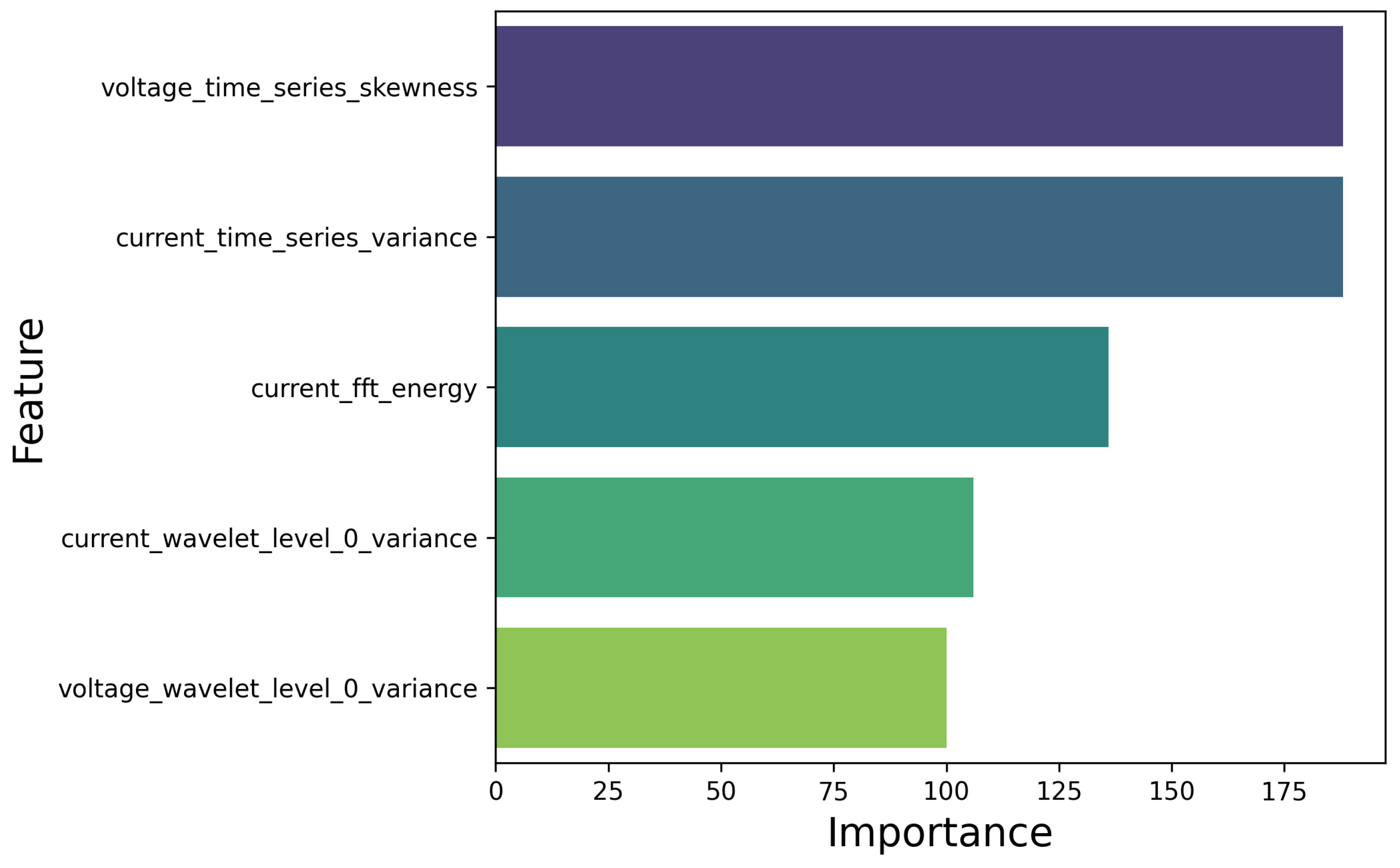
• For the INVAR36 alloy printed under the conditions of this study, feature importance revealed that the key factors were the variance in the 0–357 Hz frequency response of welding current and voltage, as well as the mean energy of the voltage FFT spectrum, highlighting the importance of frequency domain study of those signals for anomaly detection.
• The use of this model enables the development of more intelligent and automated decision-making support systems. By leveraging meaningful features and linking them to potential actions based on their values, the system can provide actionable insights. For instance, a narrow standard deviation but higher FFT energy can indicate the presence of porosity, whereas a wider standard deviation may signal process instability caused by an increased contact tip to workpiece distance.

References

1. Tao, F.; Qi, Q.; Liu, A.; Kusiak, A. Data-driven smart manufacturing. J. Manuf. Syst. 2018, 48, 157–169. [Google Scholar] [CrossRef]
2. Kusiak, A. Predictive models in digital manufacturing: Research, applications, and future outlook. Int. J. Prod. Res. 2023, 61, 6052–6062. [Google Scholar] [CrossRef]
3. Kordestani, H.; Zhang, C.; Arab, A. An Investigation into the Application of Acceleration Responses’ Trendline for Bridge Damage Detection Using Quadratic Regression. Sensors 2024, 24, 410. [Google Scholar] [CrossRef] [PubMed]
4. Kusiak, A. Smart manufacturing must embrace big data. Nature 2017, 544, 23–25. [Google Scholar] [CrossRef] [PubMed]
5. Zhang, W.; Li, Z.; Li, G.; Zhuang, P.; Hou, G.; Zhang, Q.; Li, C. Gacnet: Generate adversarial-driven cross-aware network for hyperspectral wheat variety identification. IEEE Trans. Geosci. Remote Sens. 2023, 62, 1–14. [Google Scholar] [CrossRef]
6. Yao, R.; Ge, Z.; Wang, D.; Shang, N.; Shi, J. Self-sensing joints for in-situ structural health monitoring of composite pipes: A piezoresistive behavior-based method. Eng. Struct. 2024, 308, 118049. [Google Scholar] [CrossRef]
7. Dilberoglu, U.M.; Gharehpapagh, B.; Yaman, U.; Dolen, M. The role of additive manufacturing in the era of industry 4.0. Procedia Manuf. 2017, 11, 545–554. [Google Scholar] [CrossRef]
8. Williams, S.W.; Martina, F.; Addison, A.C.; Ding, J.; Pardal, G.; Colegrove, P. Wire+ arc additive manufacturing. Mater. Sci. Technol. 2016, 32, 641–647. [Google Scholar] [CrossRef]
9. Norrish, J.; Polden, J.; Richardson, I. A review of wire arc additive manufacturing: Development, principles, process physics, implementation and current status. J. Phys. D Appl. Phys. 2021, 54, 473001. [Google Scholar] [CrossRef]
10. Priarone, P.C.; Pagone, E.; Martina, F.; Catalano, A.R.; Settineri, L. Multi-criteria environmental and economic impact assessment of wire arc additive manufacturing. CIRP Ann. 2020, 69, 37–40. [Google Scholar] [CrossRef]
11. Mattera, G.; Polden, J.; Norrish, J. Monitoring the gas metal arc additive manufacturing process using unsupervised machine learning. Weld. World 2024, 68, 2853–2867. [Google Scholar] [CrossRef]
12. Mattera, G.; Piscopo, G.; Longobardi, M.; Giacalone, M.; Nele, L. Improving the Interpretability of Data-Driven Models for Additive Manufacturing Processes Using Clusterwise Regression. Mathematics 2024, 12, 2559. [Google Scholar] [CrossRef]
13. Wu, B.; Pan, Z.; Ding, D.; Cuiuri, D.; Li, H.; Xu, J.; Norrish, J. A review of the wire arc additive manufacturing of metals: Properties, defects and quality improvement. J. Manuf. Process. 2018, 35, 127–139. [Google Scholar] [CrossRef]
14. Mattera, G.; Nele, L.; Paolella, D. Monitoring and control the Wire Arc Additive Manufacturing process using artificial intelligence techniques: A review. J. Intell. Manuf. 2023, 35, 467–497. [Google Scholar] [CrossRef]
15. Mattera, G.; Caggiano, A.; Nele, L. Optimal data-driven control of manufacturing processes using reinforcement learning: An application to wire arc additive manufacturing. J. Intell. Manuf. 2024, 1–20. [Google Scholar] [CrossRef]
16. Mattera, G.; Caggiano, A.; Nele, L. Reinforcement learning as data-driven optimization technique for GMAW process. Weld. World 2023, 68, 805–817. [Google Scholar] [CrossRef]
17. Li, Y.; Polden, J.; Pan, Z.; Cui, J.; Xia, C.; He, F.; Mu, H.; Li, H.; Wang, L. A defect detection system for wire arc additive manufacturing using incremental learning. J. Ind. Inf. Integr. 2022, 27, 100291. [Google Scholar] [CrossRef]
18. Li, W.; Zhang, H.; Wang, G.; Xiong, G.; Zhao, M.; Li, G.; Li, R. Deep learning based online metallic surface defect detection method for wire and arc additive manufacturing. Robot. Comput.-Integr. Manuf. 2023, 80, 102470. [Google Scholar] [CrossRef]
19. Alcaraz, J.Y.I.; Foqué, W.; Sharma, A.; Tjahjowidodo, T. Indirect porosity detection and root-cause identification in WAAM. J. Intell. Manuf. 2024, 35, 1607–1628. [Google Scholar] [CrossRef]
20. Li, Y.; Mu, H.; Polden, J.; Li, H.; Wang, L.; Xia, C.; Pan, Z. Towards intelligent monitoring system in wire arc additive manufacturing: A surface anomaly detector on a small dataset. Int. J. Adv. Manuf. Technol. 2022, 120, 5225–5242. [Google Scholar] [CrossRef]
21. Mattera, G.; Polden, J.; Caggiano, A.; Nele, L.; Pan, Z.; Norrish, J. Semi-supervised Learning for Real-Time Anomaly Detection in Pulsed Transfer Wire Arc Additive Manufacturing. J. Manuf. Process. 2024, 128, 84–97. [Google Scholar] [CrossRef]
22. Xia, C.; Pan, Z.; Li, Y.; Chen, J.; Li, H. Vision-based melt pool monitoring for wire-arc additive manufacturing using deep learning method. Int. J. Adv. Manuf. Technol. 2022, 120, 551–562. [Google Scholar] [CrossRef]
23. Song, H.; Li, C.; Fu, Y.; Li, R.; Zhang, H.; Wang, G. A two-stage unsupervised approach for surface anomaly detection in wire and arc additive manufacturing. Comput. Ind. 2023, 151, 103994. [Google Scholar] [CrossRef]
24. Norrish, J. Evolution of Advanced Process Control in GMAW: Innovations, Implications, and Application. Weld. Res. 2024, 103, 161–175. [Google Scholar] [CrossRef]
25. Saarela, M.; Jauhiainen, S. Comparison of feature importance measures as explanations for classification models. SN Appl. Sci. 2021, 3, 272. [Google Scholar] [CrossRef]
26. Kotsiantis, S. Feature selection for machine learning classification problems: A recent overview. Artif. Intell. Rev. 2011, 42, 157–176. [Google Scholar] [CrossRef]
27. Chen, R.C.; Dewi, C.; Huang, S.W.; Caraka, R.E. Selecting critical features for data classification based on machine learning methods. J. Big Data 2020, 7, 52. [Google Scholar] [CrossRef]
28. Chen, T.; Guestrin, C. XGBoost: A Scalable Tree Boosting System. arXiv 2016, arXiv:1603.02754. [Google Scholar] [CrossRef]
29. Pattawaro, A.; Polprasert, C. Anomaly-based network intrusion detection system through feature selection and hybrid machine learning technique. In Proceedings of the 2018 IEEE 16th International Conference on ICT and Knowledge Engineering (ICT&KE), Bangkok, Thailand, 21–23 November 2018; pp. 1–6. [Google Scholar]
30. Tian, J.; Jiang, Y.; Zhang, J.; Wang, Z.; Rodríguez-Andina, J.J.; Luo, H. High-performance fault classification based on feature importance ranking-XgBoost approach with feature selection of redundant sensor data. Curr. Chin. Sci. 2022, 2, 243–251. [Google Scholar] [CrossRef]
31. Alcaraz, J.Y.; Sharma, A.; Tjahjowidodo, T. Predicting porosity in wire arc additive manufacturing (WAAM) using wavelet scattering networks and sparse principal component analysis. Weld. World 2024, 68, 843–853. [Google Scholar] [CrossRef]
32. Mu, H.; He, F.; Yuan, L.; Commins, P.; Ding, D.; Pan, Z. A digital shadow approach for enhancing process monitoring in wire arc additive manufacturing using sensor fusion. J. Ind. Inf. Integr. 2024, 40, 100609. [Google Scholar] [CrossRef]
33. Mattera, G.; Polden, J.; Nele, L. A Time-Frequency Domain Feature Extraction Approach Enhanced by Computer Vision for Wire Arc Additive Manufacturing Monitoring Using Fourier and Wavelet Transform. J. Adv. Manuf. Syst. 2024. [Google Scholar] [CrossRef]
34. Shin, S.; Jin, C.; Yu, J.; Rhee, S. Real-time detection of weld defects for automated welding process base on deep neural network. Metals 2020, 10, 389. [Google Scholar] [CrossRef]
35. Alfaro, S.A.; Carvalho, G.; Da Cunha, F. A statistical approach for monitoring stochastic welding processes. J. Mater. Process. Technol. 2006, 175, 4–14. [Google Scholar] [CrossRef]
36. Mattera, G.; Yap, E.W.; Polden, J.; Brown, E.; Nele, L.; Duin, S.V. Utilising Unsupervised Machine Learning and IoT for Cost-Effective Anomaly Detection in multi-layer Wire Arc Additive Manufacturing. Int. J. Adv. Manuf. Technol. 2024, 135, 2957–2974. [Google Scholar] [CrossRef]
37. Mattera, G.; Vozza, M.; Polden, J.; Nele, L.; Pan, Z. Frequency Informed Convolutional Autoencoder for in situ anomaly detection in Wire Arc Additive Manufacturing. J. Intell. Manuf. 2024. [Google Scholar] [CrossRef]
38. Nigam, H.; Srivastava, H.M. Filtering of audio signals using discrete wavelet transforms. Mathematics 2023, 11, 4117. [Google Scholar] [CrossRef]
39. Gowthami, V.; Bagan, K.B.; Pushpa, S.E.P. A novel approach towards high-performance image compression using multilevel wavelet transformation for heterogeneous datasets. J. Supercomput. 2023, 79, 2488–2518. [Google Scholar] [CrossRef]
40. Yang, H.; Zhang, J.; Chen, J.; Cai, H.; Jiao, Y.; Wang, M.; Liu, E.; Li, B. Denoising of laser cladding crack acoustic emission signals based on wavelet thresholding method. J. Phys. Conf. Ser. 2024, 2713, 012069. [Google Scholar] [CrossRef]
41. Kumar, V.; Ghosh, S.; Parida, M.K.; Albert, S.K. Application of continuous wavelet transform based on Fast Fourier transform for the quality analysis of arc welding process. Int. J. Syst. Assur. Eng. Manag. 2024, 15, 917–930. [Google Scholar] [CrossRef]
42. Jang, S.; Lee, W.; Jeong, Y.; Wang, Y.; Won, C.; Lee, J.; Yoon, J. Machine learning-based weld porosity detection using frequency analysis of arc sound in the pulsed gas tungsten arc welding process. J. Adv. Join. Process. 2024, 10, 100231. [Google Scholar] [CrossRef]
43. Zhang, H.; Wu, Q.; Tang, W.; Yang, J. Acoustic Signal-Based Defect Identification for Directed Energy Deposition-Arc Using Wavelet Time–Frequency Diagrams. Sensors 2024, 24, 4397. [Google Scholar] [CrossRef] [PubMed]
44. Mattera, G.; Polden, J.; Nele, L. Monitoring Wire Arc Additive Manufacturing process of Inconel 718 thin-walled structure using wavelet decomposition and clustering analysis of welding signal. J. Adv. Manuf. Sci. Technol. 2024. [Google Scholar] [CrossRef]
45. Saito, T.; Rehmsmeier, M. The precision-recall plot is more informative than the ROC plot when evaluating binary classifiers on imbalanced datasets. PLoS ONE 2015, 10, e0118432. [Google Scholar] [CrossRef] [PubMed]
Figure 1. The pipeline that allows one to generate metal components with WAAM technology.
Mathematics 12 03414 g001
Figure 2. Experimental setup employed in this study. The robot controller communicates with the acquisition system using a TCP/IP protocol, whereas the welding machine interfaces through analog wired connections.
Mathematics 12 03414 g002
Figure 3. The images captured by the welding camera were utilized to assign labels in every 1 s length window, such as (a) defect-free deposition and (b) a layer that collapsed at the beginning. The red box highlight the layer collapse captured by welding camera.
Mathematics 12 03414 g003
Figure 4. The window of 1 s length extracted by collected data for a defect-free deposition.
Mathematics 12 03414 g004
Figure 5. Illustration of the proposed workflow for online process monitoring of the WAAM process for INVAR36.
Mathematics 12 03414 g005
Figure 6. FFT response of a 1 s voltage signal from one of the samples collected during the experimental campaign.
Mathematics 12 03414 g006
Figure 7. The decomposition levels related to a 1 s welding voltage signal from the experimental campaign, which is part of the collected dataset.
Mathematics 12 03414 g007
Figure 8. (a) Confusion matrix for LightGBM, (b) precision–recall area under the curve (PR-AUC) for LightGBM, (c) confusion matrix for XGBoost, and (d) precision–recall area under the curve (PR-AUC) for XGBoost.
Mathematics 12 03414 g008
Figure 9. The features importance score of all the most relevant features involved in anomaly detection.
Mathematics 12 03414 g009