Analysis of Neutral Implicit Stochastic Hilfer Fractional Differential Equation Involving Lévy Noise with Retarded and Advanced Arguments

Abstract

This paper investigates the qualitative properties of the solutions for neutral implicit stochastic Hilfer fractional differential equations involving Lévy noise with retarded and advanced arguments. The existence property of the solution of the aforementioned equation is demonstrated by the Mónch condition, and the uniqueness is demonstrated by the remarkable fixed point of Banach. In addition, we examine the Hyers–Ulam $\left(\mathcal{HU}\right)$ stability of the presented mathematical models. To substantiate our theoretical conclusions, a real-world example is included to illustrate their practical application.

1. Introduction

Fractional calculus $\left(\mathcal{FC}\right)$ [1] is an advanced mathematical discipline that generalizes the well-known notions of classical calculus to encompass non-integer, or fractional, orders. Unlike classical calculus, which deals exclusively with integer-order operations, $\mathcal{FC}$ offers a more flexible and comprehensive framework for the description of a wide range of phenomena. This extension has proven particularly valuable in modeling complex systems that cannot be adequately captured by standard calculus. The versatility of $\mathcal{FC}$ has led to its application across numerous fields of science and engineering [2]. In physics, for instance, it has been employed to describe anomalous diffusion and other non-standard dynamic processes [3]. In biology, $\mathcal{FC}$ has been used to model processes such as population dynamics and the spread of diseases [4]. The field has also found relevance in economics, where it aids in the modeling of financial markets and economic systems [5]. Additionally, $\mathcal{FC}$ has become increasingly important in signal processing, where it provides powerful tools for the analysis and processing of signals with complex, non-linear characteristics [6,7]. The broad applicability of $\mathcal{FC}$ underscores its significance as a versatile and essential tool in both theoretical and applied research.

Stochastic fractional differential equations ($\mathcal{SFDE}s$) are widely used to model systems influenced by random fluctuations [8]. These equations find broad application across various disciplines, such as economics, bioengineering, medicine, and biology. $\mathcal{SFDE}s$ represent a specific category of differential equations $\left(\mathcal{DE}s\right)$ that model systems influenced by both stochastic and deterministic elements. Usually, the stochastic part is depicted by a Wiener process $\left(\mathcal{WP}\right)$; these are continuous-time stochastic processes characterized by their random and unpredictable fluctuations. Kiyoshi Ito, in the 1940s, was the first to propose the use of $\mathcal{SFDE}s$ to model particle diffusion in a fluid. Since then, these equations have become essential tools in many scientific and engineering fields because they effectively capture the impact of randomness and noise on system dynamics, an important aspect in numerous physical problems.

Fractional differential equations ($\mathcal{FDE}s$) have garnered significant attention in both natural sciences and engineering due to their capability to model memory effects and hereditary properties in various processes and materials. However, many practical systems are subject to disturbances, leading to deviations from stable behavior. Therefore, it becomes critical to study $\mathcal{SFDE}s$ with impulses. Substantial advancements have been made in understanding the theory of Caputo fractional functional $\mathcal{SFDE}s$, especially regarding their stability under the Hyers–Ulam ($\mathcal{HU}$) conditions [9,10,11,12]. For instance, in [13], the authors utilized Sadovetsky’s $\mathcal{FP}$ theorem to examine neutral fractional stochastic integral differential equations that incorporate infinite delays. Despite progress, the stability analysis of such systems remains a vital area requiring further exploration [14,15,16,17,18,19,20,21]. Given the relatively limited research available on the analysis of $\mathcal{SFDE}s$ [22,23,24,25,26], there is a pressing need for more studies in this domain.

In [27], Shahid et al. explored the qualitative properties of

$$\begin{array}{c}\hfill \left\{\begin{array}{cc}& {\mathbb{D}}_{a^{+}}^p\left[{\rm Y}\left(\vartheta \right)-{\gamma }_1(\vartheta ,{{\rm Y}}_{\vartheta })\right]=\mu {\gamma }_2(\vartheta ,{{\rm Y}}_{\vartheta })+{\gamma }_3(\vartheta ,{{\rm Y}}_{\vartheta }){\displaystyle \frac{d\omega \left(\vartheta \right)}{d\vartheta }},\forall \vartheta \in [1,b],\hfill \\ & {\rm Y}\left(1\right)={\rm Y}\left(b\right)=0,\hfill \\ & {\rm Y}\left(\vartheta \right)=\varphi \left(\vartheta \right),\vartheta \in [1-m,1]\hfill \\ & {\rm Y}\left(\vartheta \right)=\phi \left(\vartheta \right),\vartheta \in [n,b+n],\hfill \end{array}\right.\end{array}$$

where ${\mathbb{D}}_{a^{+}}^p$ denotes the RL fractional derivative (FD). The functions ${\gamma }_1,{\gamma }_2,{\gamma }_3:\mathbb{J}\times \mathbb{C}([-m,n]\times \mathbb{R})\to \mathbb{R}$ are appropriately chosen functions. The term $\omega \left(\vartheta \right)$, where $\vartheta \in \mathbb{J}$, represents a Wiener process (often referred to as a stochastic process). Additionally, ${{\rm Y}}_{\vartheta }:\mathbb{C}([-m,n],\mathbb{R})\to \mathbb{R}$ is defined by ${{\rm Y}}_{\vartheta }\left(\theta \right)={\rm Y}(\vartheta +\theta )$ for $\theta \le 0$.

We are motivated by [27] and construct a new model for the analysis of neutral implicit stochastic Hilfer $\mathcal{FDE}s$ involving Lévy noise with retarded and advanced arguments:

$$\begin{array}{c}\hfill \left\{\begin{array}{c}{\mathbb{D}}_{0^{+}}^{\eta ,\beta }[\zeta \left(\xi \right)-\Psi (\xi ,{\zeta }_{\xi })]=\mu \Phi (\xi ,{\zeta }_{\xi },{\mathbb{D}}_{0^{+}}^{\eta ,\beta }\zeta \left(\xi \right))+{\rm Y}(\xi ,{\zeta }_{\xi },{\mathbb{D}}_{0^{+}}^{\eta ,\beta }\zeta \left(\xi \right)){\displaystyle \frac{dw\left(\xi \right)}{d\xi }}+{\int }_z\lambda (\xi ,{\zeta }_{\xi },z){\displaystyle \frac{d\tilde{N}(\xi ,z)}{d\xi }}\forall \xi \in (0,\varrho ]=\mathbb{J},\hfill \\ I_{0^{+}}^{1-v}[\zeta \left(0\right)-\Psi (\xi ,0)]=x_0,v=\eta +\beta -\eta \beta ,\hfill \\ \zeta \left(\xi \right)=\varphi \left(\xi \right),\xi \in [-m,0],\hfill \\ \zeta \left(\xi \right)=\phi \left(\xi \right),\xi \in [\varrho ,\varrho +n],\hfill \end{array}\right.\end{array}$$

(1)

where $D_{0^{+}}^{\eta ,\beta }$ denotes the Hilfer fractional derivative ($\mathsf{FD}$) of order $0<\eta <1$, and type 0$<\beta \le 1$ and $\Psi ,\Phi ,{\rm Y},\lambda :\mathbb{J}\times \mathbb{C}\left(\right[-m,n]\times \Re )\to \Re$ represent appropriate functions. Additionally, $w\left(\xi \right),\xi \in \mathbb{J}$, is a $\mathcal{WP}$, and ${\zeta }_{\xi }:\mathbb{C}([-m,n],\Re )\to \Re$ is defined as ${\zeta }_{\xi }\left(\theta \right)=\zeta (\xi +\theta )$ for $\theta \le 0$.

The specific outcomes of this work can be stated as follows.

• This study addresses the qualitative behavior of solutions to neutral implicit stochastic Hilfer fractional differential equations with retarded and advanced arguments influenced by Levy noise, an area with limited existing research.
• The existence and uniqueness of the solutions are established using the Monch condition and Banach’s fixed-point theorem, providing robust theoretical evidence of the model’s solvability.
• This paper examines the Hyers–Ulam stability for the proposed model and includes a real-world example to illustrate the practical application of its theoretical results, contributing to the robustness and applicability of the presented mathematical framework.

2. Supplementary Results

Here, we give some basic results so that the paper is self-contained. Let $(\Omega ,\mathbb{F},\mathbb{P})$ be the usual complete probability space. The notation ${\left({\mathcal{N}}_u\right)}_{u\ge 0}$ denotes a $\mathbf{Q}$-$\mathcal{WP}$, a stochastic process established within this probability space. The operator $\mathbf{Q}$, denoting covariance, is presumed to fulfill the condition of having a finite trace, specifically $\mathrm{Tr}\left(\mathbf{Q}\right)<\infty$. We will utilize two separable Hilbert spaces, $\mathcal{K}$ and $\mathbb{H}$. The set of all bounded linear operators from $\mathcal{K}$ to $\mathbb{H}$ is represented as $\mathcal{L}(\mathcal{K},\mathbb{H})$.

Let ${\left\{{\mu }_i\right\}}_{i=1}^{\infty }$ represent a complete orthonormal system in the Hilbert space $\mathbb{H}$. This orthonormal set is linked to a sequence ${\left\{{\varsigma }_i\right\}}_{i=1}^{\infty }$(bounded), ${\left\{{\varsigma }_i\right\}}_{i=1}^{\infty }$$\ge 0$ satisfying the relation $\mathbf{Q}{\mu }_i={\varsigma }_i{\mu }_i$ for every i. Additionally, there exists a collection of independent $\mathcal{WP}$${\left\{{\gamma }_i\right\}}_{i=1}^{\infty }$ that meet specified criteria. The stochastic process $\omega \left(\upsilon \right)$ can be formulated as follows:

$${(\omega \left(\upsilon \right),\mu )}_{\mathbb{H}}=\sum _{i=0}^{\infty }\sqrt{{\varsigma }_i}{\langle {\mu }_i,\mu \rangle }_{\mathbb{H}}{\gamma }_i\left(\upsilon \right),$$

where i ranges from 1 to m.

Subsequently, assume the set of continuous functions

$$\mathrm{C}(\mathbb{J},\mathbb{H})=\left\{\zeta :\mathbb{J}\to \mathbb{H}\mathrm{such}\mathrm{that}\zeta \mathrm{is}\mathrm{continuous}\right\}$$

such that

$${∥\zeta ∥}_{\mathbb{C}}=\underset{u\in {\mathbb{J}}_i}{sup}\mathbf{E}|u^{2-\eta }\parallel \zeta \parallel |,i=1,2,\cdots ,m=:\overline{1,m},$$

where $\mathbf{E}(.)$ represents the mathematical expectation. Let ${\mathcal{B}}_v$ denote the abstract phase space. We consider a continuous function $\xi :(-\infty ,0]\to (0,{\infty }^{+})$ that satisfies the condition $l={\int }_{-\infty }^0\xi \left(u\right)du<{\infty }^{+}$. The Hilbert space $({\mathcal{B}}_v,\parallel ·{\parallel }_{{\mathcal{B}}_v})$, induced by v, is characterized as follows:

$$\begin{array}{ccc}\hfill {\mathcal{B}}_v& =& \{\rho :(-\infty ,0)\to \mathbb{H},\mathrm{arranged}\mathrm{in}\mathrm{such}\mathrm{a}\mathrm{manner}\mathrm{that},\mathrm{for}s>0,\rho (.\left)\mathrm{is}\mathrm{measurable}\left(\mathrm{bounded}\right)\mathrm{over}\right[-s,0]\hfill \\ & & \mathrm{structured}\mathrm{in}\mathrm{such}\mathrm{a}\mathrm{way}\mathrm{that}{\int }_{-\infty }^0\xi \left(s\right)\underset{s\le \vartheta \le 0}{sup}{\left(\mathbf{E}\right|\rho \left(\vartheta \right){|}^2)}^{{\displaystyle \frac{1}{2}}}d\vartheta <{\infty }^{+}\}\hfill \end{array}$$

with

$${\parallel \rho \parallel }_{{\mathcal{B}}_v}={\int }_{-\infty }^0\xi \left(s\right)\underset{s\le \vartheta \le 0}{sup}{\left(\mathbf{E}\right|\rho \left(\vartheta \right){|}^2)}^{{\displaystyle \frac{1}{2}}}d\vartheta .$$

Definition 1 

([28]). The generalized Hilfer $\mathcal{FD}$ of order $0<\gamma <1$ and type $0\le \upsilon \le 1$ with a lower limit is denoted as

$$D_{0^{+}}^{\gamma ,\upsilon }\mathfrak{G}\left(s\right)=\left(I_{0^{+}}^{\upsilon (1-\gamma )}{\displaystyle \frac{d}{ds}}{I}_{0^{+}}^{(1-\gamma )}\mathfrak{G}\right)\left(s\right).$$

Definition 2 

([29]). Consider a stochastic process $\left\{\mathbb{X}\right(\xi )\mid \xi \ge 0\}$ defined on a complete probability space $(\Omega ,\mathbb{F},\mathbb{P})$. The process $\mathbb{X}$ is called a Lévy process if the following conditions hold:

1.

$\mathbb{X}\left(0\right)=0$;

2.

The process $\mathbb{X}$ possesses increments that are independent and identically distributed over time;

3.

$\mathbb{X}$ is stochastically continuous, meaning that, for every $a>0$ and $s>0$,

$$\underset{\xi \to s}{lim}\mathbb{P}\left(\right|\mathbb{X}\left(\xi \right)-\mathbb{X}\left(s\right)|>a)=0.$$

Lemma 1 

([30]). If $\mathcal{C}\ne \varnothing$, $\mathcal{C}\subset \mathfrak{N}$ (Banach space), $\mathcal{C}$ is closed, then $\mathcal{P}:\mathcal{C}\to \mathcal{C}$ (a contraction) has an $\mathcal{FP}$ (unique).

Lemma 2 

([31]). If $\xi \in {\mathfrak{N}}_v^{\prime }$, then ${\xi }_u\in {\mathfrak{N}}_v$, where it fulfills the following condition:

$${l(\mathbf{E}\parallel \xi \parallel }^2{)}^{{\displaystyle \frac{1}{2}}}\le \parallel {\xi }_e\parallel {\mathfrak{N}}_v\le \parallel \phi \parallel {\mathfrak{N}}_{\xi }+l\underset{s\in [0,e]}{sup}{(\mathbf{E}\parallel \varrho \left(s\right)\parallel }^2{)}^{{\displaystyle \frac{1}{2}}},$$

where $l={\int }_{-\infty }^{0}f\left(e\right)de<{\infty }^{+},$${\xi }_0=\varphi \in {\mathfrak{N}}_v.$

The Hausdorff measure of non-compactness, represented as $\varpi (·)$, is defined for any bounded $\daleth \subset \mathfrak{N}$, with $\mathfrak{N}$ being a Banach space ($\mathcal{BP}$).

$$\varpi (\daleth )=inf\{\epsilon >0;\daleth \mathrm{has}\mathrm{finite}\epsilon \mathrm{net}\mathrm{in}\mathfrak{N}\}.$$

Lemma 3 

([32]). If ℸ and ℶ are bounded subsets in $\mathfrak{N}$, then we have the following.

1.

Nonsingular: For any $x\in \mathbb{H}$ and any nonempty subset $\daleth \subset \mathbb{H}$, we have $\varpi \left(\right\{x\}\cup \daleth )=\varpi (\daleth )$.

2.

Regular: $\daleth \subset \mathbb{H}$ is precompact ⇔$\varpi (\daleth )=0$.

3.

Monotonicity: If, for bounded set ℸ and ℶ in $\mathfrak{N}$, $\daleth \subseteq \beth$, then $\varpi (\daleth )\le \varpi (\beth )$.

4.

Union Bound: $\varpi (\daleth \cup \beth )\le max\left\{\varpi \right(\daleth ),\varpi (\beth \left)\right\}$.

5.

Scaling: For any scalar μ, $\varpi (\mu \daleth )\le \left|\mu \right|\varpi (\daleth )$.

6.

Sum Property: For the sum $\daleth +\beth =\{u+v;u\in \daleth ,v\in \beth \}$, it holds that $\varpi (\daleth +\beth )\le \varpi (\daleth )+\varpi (\beth )$.

7.

Continuity: If $\mathcal{W}\subset \mathrm{C}(\mathbb{J},\mathfrak{N})$ is bounded and equicontinuous (Eqis), the function $\xi \mapsto \varpi \left(\mathcal{N}\right(u\left)\right)$ is continuous on $\mathbb{J}$.

$$\begin{array}{ccc}\hfill \varpi \left(\mathcal{N}\right)& \le & \underset{u\in \mathbb{J}}{max}\varpi \left(\mathcal{N}\left(u\right)\right),\hfill \\ \hfill \varpi \left({\int }_0^u\mathcal{N}\left(s\right)ds\right)& \le & {\int }_0^u\varpi \left(\mathcal{N}\left(s\right)\right)ds,u\in \mathbb{J},\mathrm{with}\hfill \\ \hfill {\int }_0^u\mathcal{N}\left(s\right)ds& =& {\int }_0^{u}v\left(s\right)ds,v\in \mathcal{N},u\in \mathbb{J};\hfill \end{array}$$

8.

For each $n\in \mathbb{Z}$, ${\varsigma }_i$ is a Bochner integrable function such that it maps $\mathbb{J}\to \mathfrak{N}$, and if $\parallel {\varsigma }_i\parallel \le \tilde{m}\left(u\right)$ for almost every $u\in \mathbb{J}$ for all $n\ge 1$, then the function $\chi \left(u\right)=\varpi \left({\left\{{\varsigma }_i\right\}}_{n=1}^{\infty }\right)$ is an element of $L(\mathbb{J},{\mathbb{R}}^{+})$.

$$\varpi \left(\left\{{\int }_0^u{\varsigma }_i\left(s\right)ds,n\ge 1\right\}\right)=2{\int }_0^u\chi \left(s\right)ds;$$

9.

If $\mathcal{N}$ is bounded, then, for any $\epsilon >0$, ∃${\left\{u_n\right\}}_{n=1}^{\infty }\subset \mathcal{N}$ such that $\varpi \left(\left\{u_n\right\}\right)<\epsilon$.

$$\varpi \left(\mathcal{N}\right)\le 2\varpi \left({\left\{{\varsigma }_i\right\}}_{n=1}^{\infty }\right)+\epsilon .$$

In exploring our primary findings, the aforementioned outcomes can be applied.

Lemma 4 

([33]). Let $\mathfrak{M}\subset \mathfrak{N}$ (closed and convex), containing the point 0. If $\mathfrak{F}:\mathfrak{M}\to \mathfrak{N}$ is continuous, then the set $\mathcal{M}\subset \mathfrak{N}$ is defined such that $\mathcal{M}\subset \overline{\mathrm{co}}(\left\{0\right\}\cup \mathfrak{F}\left(\mathcal{M}\right))$. This condition satisfies M$\ddot{o}$nch’s criterion, which implies that $\overline{\mathcal{M}}$ is compact. Consequently, this leads to the conclusion that there exists an $\mathcal{FP}$ of $\mathfrak{F}$ within $\mathfrak{N}$.

Lemma 5 

([34]). If $\mathbf{W}\subset \mathrm{C}([0,\varrho ],{\mathcal{L}}_2^0(\mathcal{V},X))$ and ω represents a standard $\mathcal{WP}$, then

$$\varpi \left({\int }_0^t\mathbf{W}\left(\varsigma \right)d\omega \left(\varsigma \right)\right)\le \sqrt{T.Tra\left(\mathbf{Q}\right)}\varpi \left(\mathbf{W}\left(\varsigma \right)\right),$$

with

$${\int }_0^t\mathbf{W}\left(\varsigma \right)d\omega \left(\varsigma \right)=\left\{{\int }_0^{t}v\left(\varsigma \right)d\omega \left(\varsigma \right),\mathit{for}\mathit{all}v\in \mathbf{W},t\in [0,\xi ]\right\}.$$

For convenience, Equation (1) can be written as

$$\begin{array}{ccc}\hfill {\mathbb{D}}_{0^{+}}^{\eta ,\beta }\left[\zeta \left(\xi \right)-\Psi (\xi ,{\zeta }_{\xi })\right]& =& \sigma \left(\xi \right),\forall \xi \in [0,\varrho ],\hfill \\ \hfill I_{0^{+}}^{1-v}[\zeta \left(0\right)-\Psi (\xi ,0)]=x_0,v=\eta +\beta -\eta \beta ,\\ \hfill \zeta \left(\xi \right)=\varphi \left(\xi \right),\xi \in [-m,0]\\ \hfill \zeta \left(\xi \right)=\phi \left(\xi \right)\xi \in [\varrho ,\varrho +n].\end{array}$$

(2)

Lemma 6. 

Let $0<\eta <1$ and $0<\beta \le 1$, and assume that $\sigma :\mathbb{J}\to \mathbb{H}$ is a continuous function. Then, any function $\zeta \in \mathrm{C}(\mathbb{J},\mathbb{H})$ that meets the following criteria

$$\begin{array}{ccc}\hfill {\mathbb{D}}_{0^{+}}^{\eta ,\beta }\left[\zeta \left(\xi \right)-\Psi (\xi ,{\zeta }_{\xi })\right]& =& \sigma \left(\xi \right),\forall \xi \in (0,\varrho ],\hfill \\ \hfill I_{0^{+}}^{1-v}[\zeta \left(0\right)-\Psi (\xi ,0)]=x_0,v=\eta +\beta -\eta \beta \end{array}$$

possesses the form

$$\begin{array}{cc}\hfill \zeta \left(\xi \right)& ={\displaystyle \frac{x_0}{\Gamma \left(v\right)}}{\xi }^{v-1}+\Psi (\xi ,{\zeta }_{\xi })+{\displaystyle \frac{\mu }{\Gamma \left(\eta \right)}}{\int }_0^{\xi }{(\xi -s)}^{\eta -1}\sigma \left(s\right)ds.\hfill \end{array}$$

3. Existence

Here, we formulate a series of assumptions.

$\left({\mathcal{U}}_0\right)$:

According to the following criteria, $\Phi$ functions as follows.

(i)

$\xi \in \mathbb{J}$ is the measurable, continuous function $\Phi (\xi ,m,n)$.

(ii)

${\mathcal{L}}_{\Phi }$, ${\mathcal{M}}_{\Phi },$ and ${\mathcal{N}}_{\Phi }>0$ are constants that exist such that

$$\begin{array}{c}\hfill {\mathsf{E}\parallel \Phi (\xi ,m,n)\parallel }^2\le {\mathcal{L}}_{\Phi }{(\parallel \xi \parallel }^2)+{\mathcal{M}}_{\Phi }{(\parallel m\parallel }^2)+{\mathcal{N}}_{\Phi }(\parallel n\parallel )\forall (\xi ,m,n)\in \mathbb{J}\times {\mathfrak{N}}_z.\end{array}$$

(iii)

∃${\rho }_1\in (0,\alpha )$ and $\sigma \in L^{{\displaystyle \frac{1}{{\rho }_1}}}(\mathbb{J},\Re )$ in such a way that, for bounded sets ${\Phi }_1$ and ${\Phi }_2$ in ${\mathfrak{N}}_v$, the following holds:

$$\begin{array}{c}\hfill \beta (\Phi (\xi ,{\Phi }_1,{\Phi }_2))\le \sigma \left(\xi \right)\left[sup\beta \left(({\Phi }_1,{\Phi }_2)\left(\theta \right)\right)\right].\end{array}$$

(iv)

Given the continuity of the function $\Phi$, there is a constant ${\mathcal{L}}_{\Phi }$ such that

$$\begin{array}{c}\hfill {\mathbf{E}\parallel (\Phi (\xi ,m,n)-\Phi (\xi ,u,v))\parallel }^2\le {\mathcal{L}}_{\Phi }{\parallel m-u\parallel }^2+{\mathcal{M}}_{\Phi }{\parallel n-v\parallel }^2.\end{array}$$

$\left({\mathcal{U}}_1\right)$:

$\Psi$ meets the following criteria.

(i)

$\Psi (\xi ,{\zeta }_{\xi })$ is continuous, and ${\mathcal{L}}_{\Psi }>0$ exists in such a way that

$$\begin{array}{c}\hfill \mathbf{E}{∥\Psi (\xi ,{\zeta }_{\xi })∥}^2\le {\mathcal{L}}_{\Psi }{(1+\parallel \zeta \parallel }^2).\end{array}$$

(ii)

${\mathcal{L}}_{\Psi }$ (a constant) exists in such a way that

$$\begin{array}{c}\hfill \mathbf{E}\parallel (\Psi (\xi ,\overline{u})-\Psi (\xi ,\overline{v})){\parallel }^2\le {\mathcal{L}}_{\Psi }{\parallel \overline{u}-\overline{v}\parallel }^2.\end{array}$$

(iii)

∃${\rho }_2\in (0,\alpha )$ and $\Psi \in L^{{\displaystyle \frac{1}{{\rho }_2}}}(\mathbb{J},\Re )$, and, for ${\Psi }_2$ (bounded) contained in ${\mathfrak{N}}_v$, the following holds:

$$\begin{array}{c}\hfill \beta (\Psi (\xi ,{\Psi }_2))\le {\Psi }^{\prime }\left(\xi \right)\left[sup\beta \left({\Psi }_2\left(\theta \right)\right)\right],\mathrm{where}\mathcal{G}=\underset{\xi \in \mathbb{J}}{sup}{\Psi }^{\prime }\left(t\right).\end{array}$$

$\left({\mathcal{U}}_2\right)$:

The function ${\rm Y}$ adheres to the following.

(i)

A constant ${\rho }_3\in (0,\alpha )$ exists, along with $l_2\in L^{{\displaystyle \frac{1}{{\rho }_3}}}(\mathsf{j},\Re )$ and ${\Omega }_2:\Re \to \Re$ (integrable), fulfilling

$$\begin{array}{c}\hfill \mathbf{E}{∥{\rm Y}(\xi ,m,n)∥}^2\le l_1\left(\xi \right){\Omega }_1(\parallel m\parallel )+l_2(\parallel n\parallel ),\end{array}$$

where ${\Omega }_1$ satisfies the requirement that ${lim}_{\xi \to \infty }inf{\displaystyle \frac{{\Omega }_1\left(\xi \right)}{\xi }}=0$.

(ii)

∃${\mathcal{L}}_{{\rm Y}}$ (a constant) and a positive constant ${\mathcal{M}}_{{\rm Y}}>0$ in such a way that

$${\mathbf{E}\parallel {\rm Y}(\xi ,m,n)-{\rm Y}(\xi ,u,v)\parallel }^2\le {\mathcal{L}}_{{\rm Y}}{\mathsf{E}\parallel m-u\parallel }^2+{\mathcal{M}}_{{\rm Y}}\mathsf{E}{\parallel n-v\parallel }^2$$

(iii)

∃${\rho }_4\in (0,\alpha )$ and ${\sigma }_1\in L^{{\displaystyle \frac{1}{{\rho }_4}}}(\mathbb{J},\Re )$, in such a way that, for bounded sets ${{\rm Y}}_3$ and ${{\rm Y}}_4$ within ${\mathfrak{N}}_v$, the following holds:

$$\begin{array}{c}\hfill \beta ({\rm Y}(\xi ,{{\rm Y}}_3,{{\rm Y}}_4))\le {\sigma }_1\left(\xi \right)\left[sup\beta \left(({{\rm Y}}_3,{{\rm Y}}_4)\left(\theta \right)\right)\right].\end{array}$$

$\left({\mathcal{U}}_3\right)$:

The function $\lambda$ adheres to the following.

(i)

$\lambda (\xi ,m)$ is measurable and continuous for almost all $\xi \in \mathbb{J}.$

(ii)

A constant ${\mathcal{L}}_{\lambda }>0$ exists such that the following condition is satisfied:

$$\begin{array}{c}\hfill {\mathsf{E}\parallel \lambda (\xi ,m)\parallel }^2\le {\mathcal{L}}_{\lambda }{(1+\parallel m\parallel }^2)\forall (\xi ,m)\in \mathbb{J}\times {\mathfrak{N}}_z.\end{array}$$

(iii)

∃$\sigma \in L^{{\displaystyle \frac{1}{{\rho }_1}}}(\mathbb{J},\Re )$ and ${\rho }_1\in (0,\alpha )$ are known to exist, in such a way that, for any ${\lambda }_1\subset {\mathfrak{N}}_v$ (bounded set),

$$\begin{array}{c}\hfill \beta (\lambda (\xi ,{\lambda }_1))\le \sigma \left(\xi \right)\left[sup\beta \left({\lambda }_1\left(\theta \right)\right)\right].\end{array}$$

(iv)

Given the continuous nature of the function $\lambda$, there is a constant ${\mathcal{L}}_{\lambda }$ satisfying

$$\begin{array}{c}\hfill {\mathbf{E}\parallel (\lambda (\xi ,m)-\lambda (\xi ,u))\parallel }^2={\mathcal{L}}_{\lambda }{\parallel m-u\parallel }^2.\end{array}$$

$\left({\mathcal{U}}_4\right)$:

$$\begin{array}{c}\hfill \left({\mathcal{L}}_{\Psi }+{\displaystyle \frac{{\rho }^{2\eta -1}}{\Gamma {\left(\eta \right)}^2(2\eta -1)}}[{\mu }^2{\mathcal{M}}_{\Phi }+{\mathcal{L}}_{\lambda }]\right)l^2<1,\end{array}$$

$$\begin{array}{c}\hfill \Delta =\left(\mathcal{G}+{\displaystyle \frac{\mu {\rho }^{\eta }}{\Gamma (\eta +1)}}\parallel {\sigma }_1\parallel +{\displaystyle \frac{\sqrt{Tr\left(\mathcal{Q}\right)}{\rho }^{\eta +\frac{1}{2}}}{\Gamma (\eta +1)}}\parallel {\sigma }_2\parallel +{\displaystyle \frac{{\rho }^{\eta }}{\Gamma (\eta +1)}}\parallel {\sigma }_3\parallel \right)<1,\end{array}$$

and

$$\begin{array}{cc}\hfill {\Delta }_1=& 3\{{\mathcal{L}}_{\Psi }+{\displaystyle \frac{3{\rho }^{2\eta }}{\Gamma \left(\eta \right)(2\eta -1)}}[\left({\mu }^2{\mathcal{L}}_{\Phi }+Tr\left(\mathcal{Q}\right){\mathcal{L}}_{{\rm Y}}+{\mathcal{L}}_{\lambda }\right)\hfill \\ \hfill & +3\left({\mu }^2{\mathcal{L}}_{\Psi }+Tr\left(\mathcal{Q}\right){\mathcal{M}}_r)\right){\displaystyle \frac{{\mathcal{L}}_{\Psi }+{\mu }^2{\mathcal{L}}_{\Phi }+{\mathcal{L}}_{\lambda }+Tr\left(\mathcal{Q}\right)}{1-{\mu }^2{\mathcal{L}}_{\Psi }-Tr\left(\mathcal{Q}\right){\mathcal{L}}_r}}\left]\right\}<1.\hfill \end{array}$$

Lemma 7. 

Let $\mathcal{X}$ be a closed convex subset of $\mathfrak{N}$ such that $0\in \mathcal{X}$. Consider a continuous mapping $𝘍:\mathcal{X}\to \mathfrak{N}$ that satisfies M$\ddot{o}$nch’s condition: for any countable set $\mathbf{M}\subset \mathcal{X}$, if $\mathbf{M}\subset \overline{\mathrm{co}}(0\cup 𝘍\left(\mathbf{M}\right))$, $\overline{\mathbf{M}}$ is compact. Under these circumstances, an $\mathcal{FP}$ for 𝘍 must exist within $\mathcal{X}$.

Theorem 1. 

Let $\left({\mathcal{U}}_0\right)-\left({\mathcal{U}}_3\right)$ be fulfilled; then, in $[-m,\varrho +n]$, (2) has at least one solution.

Proof. 

First, we need to express problem (2) as a fixed-point problem and introduce an appropriate operator. Define $\mathbb{H}$ as an operator that maps $\mathbb{C}\left(\right[-m,\varrho +n],\Re )$ to itself, specified by

$$\begin{array}{c}\hfill \mathbb{H}\zeta \left(\xi \right)=\left\{\begin{array}{cc}& \varphi \left(\xi \right),\mathrm{if}\xi \in [-m,0],\hfill \\ & {\displaystyle \frac{x_0}{\Gamma \left(v\right)}}{\xi }^{v-1}+\Psi (\xi ,{\zeta }_t)+{\displaystyle \frac{1}{\Gamma \left(\eta \right)}}{\int }_0^{\xi }{(\xi -s)}^{\eta -1}\sigma \left(s\right)ds,\mathrm{if}\xi \in [0,\varrho ],\hfill \\ & \phi \left(\xi \right),\mathrm{if}\xi \in [\varrho ,\varrho +n].\hfill \end{array}\right.\end{array}$$

(3)

Let $x:[-m,\varrho +n]’\to \Re$ satisfy

$$\begin{array}{c}\hfill x\left(\xi \right)=\left\{\begin{array}{cc}& \varphi \left(\xi \right),\mathrm{if}\xi \in [-m,0],\hfill \\ & 0,\mathrm{if}\xi \in [0,\varrho ],\hfill \\ & \phi \left(\xi \right),\mathrm{if}\xi \in [\varrho ,\varrho +n].\hfill \end{array}\right.\end{array}$$

(4)

For every $z\in \mathbb{C}\left(\right[0,\varrho ],\Re )$, we define the function u as

$$\begin{array}{c}\hfill u\left(\xi \right)=\left\{\begin{array}{cc}& 0,\mathrm{if}\xi \in [1-r,1]\hfill \\ & z\left(\xi \right),\mathrm{if}\xi \in [0,\varrho ]\hfill \\ & 0,\mathrm{if}\xi \in [\varrho ,\varrho +n].\hfill \end{array}\right.\end{array}$$

(5)

Let us set $\zeta \left(\xi \right)=z\left(\xi \right)+x\left(\xi \right)$ such that ${\zeta }_{\xi }=z_{\xi }+x_{\xi }$ for every $\xi \in [0,\varrho ]$, where

$$\begin{array}{cc}\hfill \zeta \left(\xi \right)& ={\displaystyle \frac{x_0}{\Gamma \left(v\right)}}{\rho }^{v-1}+\Psi (\xi ,{\zeta }_{\xi })+{\displaystyle \frac{\mu }{\Gamma \left(\eta \right)}}{\int }_0^{\xi }{(\xi -s)}^{\eta -1}\Phi (s,{\zeta }_s,{\mathbb{D}}_{0^{+}}^{\eta ,\beta }{\zeta }_s)ds+{\displaystyle \frac{1}{\Gamma \left(\eta \right)}}{\int }_0^{\xi }{(\xi -s)}^{\eta -1}{\rm Y}(s,{\zeta }_s,{\mathbb{D}}_{0^{+}}^{\eta ,\beta }{\zeta }_s)dw\left(s\right)\hfill \\ \hfill & +{\displaystyle \frac{1}{\Gamma \left(\eta \right)}}{\int }_0^{\xi }{(\xi -s)}^{\eta -1}({\int }_z\lambda (\xi ,{\zeta }_{x}i,z)\tilde{N}(d\xi ,dz)).\hfill \end{array}$$

$$\begin{array}{cc}\hfill z\left(\xi \right)& ={\displaystyle \frac{x_0}{\Gamma \left(v\right)}}{\rho }^{v-1}+\Psi (\xi ,z_t+x_t)+{\displaystyle \frac{\mu }{\Gamma \left(\eta \right)}}{\int }_0^{\xi }{(\xi -s)}^{\eta -1}\Phi (s,z_s+x_s,{\mathbb{D}}_{0^{+}}^{\eta ,\beta }{\zeta }_s)ds+{\displaystyle \frac{1}{\Gamma \left(\eta \right)}}{\int }_0^{\xi }{(\xi -s)}^{\eta -1}{\rm Y}(s,z_s+x_s,{\mathbb{D}}_{0^{+}}^{\eta ,\beta }{\zeta }_s)dw\left(s\right)\hfill \\ \hfill & +{\displaystyle \frac{1}{\Gamma \left(\eta \right)}}{\int }_0^{\xi }{(\xi -s)}^{\eta -1}({\int }_z\lambda (\xi ,{\zeta }_{\xi },z)\tilde{N}(d\xi ,dz)).\hfill \end{array}$$

Now, let $\mathfrak{N}=\{z\in \mathbb{C}([-m,\varrho +n],\Re \left)\right\}$, $\beth :\mathfrak{N}\to \mathfrak{N}$ be such that

$$\begin{array}{c}\hfill (\beth z)\left(\xi \right)=\left\{\begin{array}{c}0,if\xi \in [-m,0),\hfill \\ {\displaystyle \frac{x_0}{\Gamma \left(v\right)}}{\rho }^{v-1}+\Psi (\xi ,z_{\xi }+x_{\xi })+{\displaystyle \frac{\mu }{\Gamma \left(\eta \right)}}{\int }_0^{\xi }{(\xi -s)}^{\eta -1}\Phi (s,z_s+x_s,{\mathbb{D}}_{0^{+}}^{\eta ,\beta }{\zeta }_s)ds\hfill \\ +{\displaystyle \frac{1}{\Gamma \left(\eta \right)}}{\int }_0^{\xi }{(\xi -s)}^{\eta -1}{\rm Y}(s,z_s+x_s,{\mathbb{D}}_{0^{+}}^{\eta ,\beta }{\zeta }_s)dw\left(s\right)+{\displaystyle \frac{1}{\Gamma \left(\eta \right)}}{\int }_0^{\xi }{(\xi -s)}^{\eta -1}({\int }_z\lambda (\xi ,z_{\xi }+x_{\xi },z)\tilde{N}(d\xi ,dz)).\hfill \\ 0,if\xi [\varrho ,\varrho +n].\hfill \end{array}\right.\end{array}$$

(6)

Let ${\mathfrak{N}}_v={\{z\in \mathbb{C}([-m,\varrho +n],\Re ):\parallel z\parallel }_{[-m,\varrho +n]}\le v\}$.

For $z\in \mathfrak{N}$ and $s\in \mathbb{J}$, the following holds:

$$\begin{array}{ccc}\hfill \parallel z_s+x_s\parallel & \le & \parallel z_s{\parallel }_{[-m,n]}+\parallel x_s{\parallel }_{[-m,n]}\le l\underset{[0,\varrho ]}{sup}\mathbf{E}\left(\right|s^{2-\eta }{\parallel z\left(s\right)\parallel |}^2{|}^{{\displaystyle \frac{1}{2}}})+\parallel x_s{\parallel }_{[0,\varrho ]}\hfill \\ & =& lv+\parallel x_s{\parallel }_{[0,\varrho ]}=v^{\prime }\hfill \end{array}$$

Step 1. We are assured that we can find v that satisfies $\beth \left({\mathfrak{N}}_v\right)\subset {\mathfrak{N}}_v$. Assume, as a contradiction, that no such v exists. Then, for every positive integer v, there is a function $z_v\in {\mathfrak{N}}_v$ such that $\parallel \beth z_v{\parallel }^2>v^2$. However, according to the assumptions, it follows that

$$\begin{array}{cc}\hfill \mathbf{E}|\parallel (\beth z_v){\parallel |}^2\le & \mathbf{E}\left|\right|{\displaystyle \frac{x_0}{\Gamma \left(v\right)}}{\rho }^{v-1}{\left|\right|}^2+\mathbf{E}\left|\right|\Psi (\xi ,z_{\xi }+x_{\xi }){\left|\right|}^2+\mathbf{E}\left|\right|{\displaystyle \frac{\mu }{\Gamma \left(\eta \right)}}{\int }_0^{\xi }{(\xi -s)}^{\eta -1}\Phi (s,z_s+x_s,{\mathbb{D}}_{0^{+}}^{\eta ,\beta }{z}_s)ds{\left|\right|}^2\hfill \\ \hfill & +\mathbf{E}\left|\right|{\displaystyle \frac{1}{\Gamma \left(\eta \right)}}{\int }_0^{\xi }{(\xi -s)}^{\eta -1}{\rm Y}(s,z_s+x_s,{\mathbb{D}}_{0^{+}}^{\eta ,\beta }{z}_s)dw\left(s\right){\left|\right|}^2\hfill \\ \hfill & +\mathbf{E}\left|\right|{\displaystyle \frac{1}{\Gamma \left(\eta \right)}}{\int }_0^{\xi }{(\xi -s)}^{\eta -1}({\int }_z\lambda (t,z_{\xi }+x_{\xi },z)\tilde{N}(dt,dz)){\left|\right|}^2.\hfill \end{array}$$

Applying the Cauchy–Schwarz inequality along with assumptions ${\mathcal{U}}_0$ to ${\mathcal{U}}_3$, we obtain the following result.

$$\begin{array}{cc}\hfill \le & \mathbf{E}\left|\right|{\displaystyle \frac{x_0}{\Gamma \left(v\right)}}{\rho }^{v-1}{\left|\right|}^2+{\mathcal{L}}_{\Psi }+{\mathcal{L}}_{\Psi }{\left(\acute{v}\right)}^2+{\displaystyle \frac{{\rho }^{2\eta }}{\Gamma \left({\eta }^2\right)(2\eta -1)}}[{\mu }^2{\mathcal{L}}_{\Phi }\left(s\right)+{\mathcal{L}}_{{\rm Y}}\left(s\right)+{\mathcal{L}}_{\lambda }+{\mathcal{M}}_{\Phi }{\left(\acute{v}\right)}^2+{\mathcal{M}}_{{\rm Y}}{l}_{{\rm Y}}\left(\xi \right){\Omega }_1{\left(\acute{v}\right)}^2\hfill \\ & +{\mathcal{L}}_{\lambda }{\left(\acute{v}\right)}^2+\left({\mu }^2{\mathcal{N}}_{\Phi }+{\mathcal{N}}_{{\rm Y}}\right)\times \left|\right|{\mathbb{D}}^{\eta ,\beta }{\zeta }_s{\left|\right|}^2]\hfill \\ \hfill \le & \mathbf{E}\left|\right|{\displaystyle \frac{x_0}{\Gamma \left(v\right)}}{\rho }^{v-1}{\left|\right|}^2+{\mathcal{L}}_{\Psi }+{\mathcal{L}}_{\Psi }{\left(\acute{v}\right)}^2+{\displaystyle \frac{{\rho }^{2\eta }}{\Gamma \left({\eta }^2\right)(2\eta -1)}}[{\mu }^2{\mathcal{L}}_{\Phi }\left(s\right)+{\mathcal{L}}_{{\rm Y}}\left(s\right)+{\mathcal{L}}_{\lambda }+{\mathcal{M}}_{\Phi }{\left(\acute{v}\right)}^2+{\mathcal{M}}_{{\rm Y}}{l}_{{\rm Y}}\left(\xi \right){\Omega }_1{\left(\acute{v}\right)}^2\hfill \\ & +{\mathcal{L}}_{\lambda }{\left(\acute{v}\right)}^2+\left({\mu }^2{\mathcal{N}}_{\Phi }+{\mathcal{N}}_{{\rm Y}}\right)\times {\displaystyle \frac{{\mathcal{L}}_{\Psi }+{\mu }^2{\mathcal{L}}_{\Phi }\left(\xi \right)+{\mathcal{L}}_{{\rm Y}}\left(s\right)+{\mathcal{L}}_{\lambda }\left(s\right)+({\mathcal{L}}_{\lambda }+{\mathcal{L}}_{\Psi }){\left(\acute{v}\right)}^2}{1-{\mathcal{N}}_{\Phi }-{\mathcal{N}}_{{\rm Y}}}}].\hfill \end{array}$$

Therefore, we obtain

$$\begin{array}{cc}\hfill v^2& <\left|\right|\beth z_v|{|}^2\hfill \\ \hfill \le & \mathbf{E}\left|\right|{\displaystyle \frac{x_0}{\Gamma \left(v\right)}}{\rho }^{v-1}{\left|\right|}^2+{\mathcal{L}}_{\Psi }+{\mathcal{L}}_{\Psi }{\left(\acute{v}\right)}^2+{\displaystyle \frac{{\rho }^{2\eta }}{\Gamma \left({\eta }^2\right)(2\eta -1)}}[{\mu }^2{\mathcal{L}}_{\Phi }\left(s\right)+{\mathcal{L}}_{{\rm Y}}\left(s\right)\hfill \\ \hfill & +{\mathcal{L}}_{\lambda }+{\mathcal{M}}_{\Phi }{\left(\acute{v}\right)}^2+{\mathcal{M}}_{{\rm Y}}{l}_{{\rm Y}}\left(\xi \right){\Omega }_1{\left(\acute{v}\right)}^2+{\mathcal{L}}_{\lambda }{\left(\acute{v}\right)}^2+\left({\mu }^2{\mathcal{N}}_{\Phi }+{\mathcal{N}}_{{\rm Y}}\right)\times {\displaystyle \frac{{\mathcal{L}}_{\Psi }+{\mu }^2{\mathcal{L}}_{\Phi }\left(\xi \right)+{\mathcal{L}}_{{\rm Y}}\left(s\right)+{\mathcal{L}}_{\lambda }\left(s\right)+({\mathcal{L}}_{\lambda }+{\mathcal{L}}_{\Psi }){\left(\acute{v}\right)}^2}{1-{\mathcal{N}}_{\Phi }-{\mathcal{N}}_{{\rm Y}}}}].\hfill \end{array}$$

With $v\to \infty$, we have

$$\underset{v\to \infty }{lim}{\displaystyle \frac{v^{\prime }}{v}}=\underset{v\to \infty }{lim}{\displaystyle \frac{lv+\parallel x_s\parallel }{v}}=l\mathrm{and}\underset{\xi \to \infty }{lim}inf{\displaystyle \frac{{\Omega }_1\left(\xi \right)}{\xi }}=0,$$

which implies

$$\begin{array}{c}\hfill \left({\mathcal{L}}_{\Psi }+{\displaystyle \frac{{\rho }^{2\eta -1}}{\Gamma {\left(\eta \right)}^2(2\eta -1)}}[{\mu }^2{\mathcal{M}}_{\Phi }+{\mathcal{L}}_{\lambda }]\right)l^2>1.\end{array}$$

This clearly contradicts assumption $\left({\mathcal{U}}_4\right)$. Therefore, for a certain value of v, we have $\beth \left({\mathfrak{N}}_v\right)\subset {\mathfrak{N}}_v$.

Step 2. If $\left\{z_n\right\}$ is a sequence in ${\mathfrak{N}}_v$ that converges to z in ${\mathfrak{N}}_v$, then

$$\begin{array}{cc}\hfill \mathbf{E}\parallel (\beth z_n)\left(\xi \right)-(\beth z)\left(\xi \right){\parallel }^2\le & 3\mathbf{E}\parallel (\Psi (\xi ,z_n+x_{\xi })-\Psi (\xi ,z_{\xi }+x_{\xi })){\parallel }^2\hfill \\ \hfill & +3\mu \mathbf{E}\parallel {\displaystyle \frac{1}{\Gamma \left(\eta \right)}}{\int }_0^{\xi }{(\xi -s)}^{\eta -1}(\Phi (s,z_{ns}+x_s,{\mathbb{D}}^{\eta ,\beta }{z}_n)-\Phi (s,z_s+x_s),{\mathbb{D}}^{\eta ,\beta }z){ds\parallel }^2\hfill \\ \hfill & +3\mathbf{E}\parallel {\displaystyle \frac{1}{\Gamma \left(\eta \right)}}{\int }_0^{\xi }{(\xi -s)}^{\eta -1}[{\rm Y}(s,z_{ns}+x_s,{\mathbb{D}}^{\eta ,\beta }{z}_n)-{\rm Y}(s,z_s+x_s,{\mathbb{D}}^{\eta ,\beta }z)]dw\left(s\right){\parallel }^2\hfill \\ \hfill & +3\mathbf{E}{∥{\displaystyle \frac{1}{\Gamma \left(\eta \right)}}{\int }_0^{\xi }{(\xi -s)}^{\eta -1}[{\int }_z\lambda (s,z_{ns}+x_s)-\lambda (s,z_s+x_s)]\tilde{N}(dt,dz)∥}^2\hfill \\ \hfill \le & 3{\mathcal{L}}_{\Psi }\left|\right|z_n-{z\left|\right|}^2+{\displaystyle \frac{3{\rho }^{2\eta }}{\Gamma \left(\eta \right)(2\alpha -1)}}[\left({\mu }^2{\mathcal{L}}_{\Phi }+Tr\left(\mathcal{Q}\right){\mathcal{L}}_{{\rm Y}}+{\mathcal{L}}_{\lambda }\right)\left|\right|z_n-z{\left|\right|}^2\hfill \\ \hfill & +3\left({\mu }^2{\mathcal{L}}_{\Psi }+Tr\left(\mathcal{Q}\right){\mathcal{M}}_{{\rm Y}}\right)\left|\right|{\mathbb{D}}^{\eta ,\beta }{z}_n-z{\left|\right|}^2]\hfill \\ \hfill \le & 3{\mathcal{L}}_{\Psi }\left|\right|z_n-z{\left|\right|}^2+{\displaystyle \frac{3{\rho }^{2\rho }}{\Gamma \left(\eta \right)(2\alpha -1)}}[\left({\mu }^2{\mathcal{L}}_{\Phi }+Tr\left(\mathcal{Q}\right){\mathcal{L}}_{{\rm Y}}+{\mathcal{L}}_{\lambda }\right)\hfill \\ \hfill & +3\left({\mathcal{L}}_{\Psi }+Tr\left(\mathcal{Q}\right){\mathcal{M}}_{{\rm Y}}\right){\displaystyle \frac{{\mathcal{L}}_{\Psi }+{\mu }^2{\mathcal{L}}_{\Phi }+{\mathcal{L}}_{\lambda }+Tr\left(\mathcal{Q}\right){\mathcal{M}}_{{\rm Y}}}{1-{\mu }^2{\mathcal{L}}_{\Phi }-Tr\left(\mathcal{Q}\right){\mathcal{M}}_{{\rm Y}}}}\left]\right||z_n-z{\left|\right|}^2\hfill \\ \hfill & \to 0\mathrm{for}n\to \infty .\hfill \end{array}$$

Consequently,

$$\begin{array}{c}\hfill ∥\beth z_n-\beth z∥\to 0\mathrm{for}n\to \infty ,\end{array}$$

Step 3. For any ${\xi }_1,{\xi }_2\in [0,\varrho ]$ with ${\xi }_1<{\xi }_2$, it follows that

$$\begin{array}{cc}\hfill \mathbf{E}{\left|{\xi }^{2-\eta }∥(\beth z)\left({\xi }_2\right)-(\beth z)\left({\xi }_1\right)∥\right|}^2\le & {\mathcal{K}}_1^2\left({\xi }_1\right)\mathsf{E}|{\xi }^{2-\eta }\parallel \beth z\left({\xi }_1\right)-\beth z\left({\xi }_2\right)\parallel {|}^2\hfill \\ \hfill \le & {\mathcal{K}}_1^2\left({\xi }_1\right)\mathbf{E}{\parallel {\xi }_1^{2-\eta }\beth z\left({\xi }_1\right)-{\xi }_2^{2-\eta }\beth z\left({\xi }_2\right)\parallel }^2\hfill \\ \hfill & +{\mathcal{K}}_1^2\left({\xi }_1\right)\mathbf{E}{\parallel {\xi }_2^{2-\eta }\beth z\left({\xi }_2\right)-{\xi }_2^{2-\eta }\beth z\left({\xi }_2\right)\parallel }^2\hfill \\ \hfill \le & {\mathcal{K}}_1^2\left({\xi }_1\right)\mathbf{E}{\parallel {\xi }_1^{2-\eta }\beth z\left({\xi }_1\right)-{\xi }_2^{2-\eta }\beth z\left({\xi }_2\right)\parallel }^2\hfill \\ \hfill & +{\mathcal{K}}_1^2\left({\xi }_1\right)\mathbf{E}\parallel \beth z\left({\xi }_2\right){\parallel }^2{\parallel {\xi }_2^{2-\eta }-{\xi }_1^{2-\eta }\parallel }^2.\hfill \end{array}$$

(7)

As ${\xi }_2\to {\xi }_1$, the right-hand side of (7) approaches zero, i.e.,

$$\mathbf{E}|{\xi }^{2-\eta }\parallel (\beth z)\left({\xi }_2\right)-(\beth z)\left({\xi }_1\right)\parallel {|}^2\to 0.$$

This indicates that ℶ is Eqis.

Step 4. Let $\beth ={\beth }_1+{\beth }_2+{\beth }_3+{\beth }_4$, with

$$\begin{array}{cc}\hfill {\beth }_1\left(z\right)\left(t\right)& =\Psi (\xi ,z_{\xi }+x_{\xi }),\hfill \\ \hfill {\beth }_2\left(z\right)\left(t\right)& ={\displaystyle \frac{\mu }{\Gamma \left(\eta \right)}}{\int }_0^{\xi }{(\xi -s)}^{\eta -1}\Phi (s,z_s+x_s,{\mathbb{D}}_{0^{+}}^{\eta ,\beta }{\zeta }_s)ds\hfill \\ \hfill {\beth }_3\left(z\right)\left(t\right)& ={\displaystyle \frac{1}{\Gamma \left(\eta \right)}}{\int }_0^{\xi }{(\xi -s)}^{\alpha -1}{\rm Y}(s,z_s+x_s,{\mathbb{D}}_{0^{+}}^{\eta ,\beta }{\zeta }_s)dw\left(s\right)\hfill \\ \hfill {\beth }_4\left(z\right)\left(t\right)& ={\displaystyle \frac{1}{\Gamma \left(\eta \right)}}{\int }_0^{\xi }{(\xi -s)}^{\alpha -1}({\int }_z\lambda (t,z_{\xi }+x_{\xi },z)\tilde{N}(dt,dz)).\hfill \end{array}$$

Assume that $\mathcal{W}\subset {\mathfrak{N}}_v$ is a countable set and that $\mathcal{W}\subset \overline{\mathrm{co}}(0\cup \beth \left(\mathcal{W}\right))$. Our objective is to demonstrate that $\beta \left(\mathcal{W}\right)=0$. Let $\mathcal{W}={\left\{z_n\right\}}_{n=1}^{\infty }$ be a sequence drawn from $\mathcal{W}$. Since $\beth \left(\mathcal{W}\right)$ is Eqis on $\mathbb{C}[-m,\varrho +n]$, it follows that $\mathcal{W}\subset \overline{\mathrm{co}}(0\cup \beth \left(\mathcal{W}\right))$ is also Eqis on $\mathbb{C}[-m,\varrho +n]$.

By utilizing Lemma 1, Lemma 3, and $\left({\mathcal{U}}_0\right)-\left({\mathcal{U}}_3\right)$, we can conclude that

$$\begin{array}{cc}\hfill \Lambda \left({\left\{{\beth }_1{z}_n\left(\xi \right)\right\}}_{n=1}^{\infty }\right)& \le \Lambda (\Psi (\xi ,z_{n\xi }+x_{\xi }))\hfill \\ \hfill & \le \mathcal{G}sup\Lambda \left({\left\{z_{n\xi }(\beth )\right\}}_{n=1}^{\infty }\right).\hfill \end{array}$$

(8)

$$\begin{array}{cc}\hfill \Lambda \left({\left\{{\beth }_2{z}_n\left(\xi \right)\right\}}_{n=1}^{\infty }\right)& \le {\displaystyle \frac{\mu }{\Gamma \left(\eta \right)}}{\int }_0^{\xi }{(\xi -s)}^{\eta -1}{\sigma }_1\left(s\right)\left[sup\Lambda \left({\left\{z_{ns}(\beth )\right\}}_{n=1}^{\infty }\right)\right]ds\hfill \\ \hfill & \le {\displaystyle \frac{\mu {\xi }^{\eta }}{\Gamma (\eta +1)}}\parallel {\sigma }_1\parallel sup\Lambda \left({\left\{z_{ns}(\beth )\right\}}_{n=1}^{\infty }\right)\hfill \end{array}$$

(9)

$$\begin{array}{cc}\hfill \Lambda \left({\left\{{\beth }_3{z}_n\left(\xi \right)\right\}}_{n=1}^{\infty }\right)& \le {\displaystyle \frac{2\sqrt{Tr\left(\mathcal{Q}\right).T}}{\Gamma \eta }}{\int }_0^{\xi }{(\xi -s)}^{\eta -1}{\sigma }_2\left(s\right)\left[sup\Lambda \left({\left\{z_{ns}(\beth )\right\}}_{n=1}^{\infty }\right)\right]ds\hfill \\ \hfill & \le {\displaystyle \frac{2\sqrt{Tr\left(\mathcal{Q}\right)}{\xi }^{\eta +\frac{1}{2}}}{\Gamma \eta +1}}\parallel {\sigma }_2\parallel sup\Lambda \left({\left\{z_{ns}(\beth )\right\}}_{n=1}^{\infty }\right)\hfill \end{array}$$

(10)

$$\begin{array}{cc}\hfill \Lambda \left({\left\{{\beth }_4{z}_n\left(\xi \right)\right\}}_{n=1}^{\infty }\right)& \le {\displaystyle \frac{1}{\Gamma \left(\eta \right)}}{\int }_0^{\xi }{(\xi -s)}^{\eta -1}{\sigma }_3\left(s\right)\left[sup\Lambda \left({\left\{z_{ns}(\beth )\right\}}_{n=1}^{\infty }\right)\right]ds\hfill \\ \hfill & \le {\displaystyle \frac{{\xi }^{\eta }}{\Gamma (\eta +1)}}\parallel {\sigma }_3\parallel sup\Lambda \left({\left\{z_{ns}(\beth )\right\}}_{n=1}^{\infty }\right)\hfill \end{array}$$

(11)

Finally, we obtain

$$\begin{array}{cc}\hfill \Lambda \left({\left\{z_n(\beth )\right\}}_{n=1}^{\infty }\right)\le & \Lambda \left({\left\{{\beth }_1{z}_n\left(t\right)\right\}}_{n=1}^{\infty }\right)+\Lambda \left({\left\{{\beth }_2{z}_n\left(t\right)\right\}}_{n=1}^{\infty }\right)+\Lambda \left({\left\{{\beth }_3{z}_n\left(t\right)\right\}}_{n=1}^{\infty }\right)+\Lambda \left({\left\{{\beth }_4{z}_n\left(t\right)\right\}}_{n=1}^{\infty }\right)\hfill \\ \hfill \le & \mathcal{G}sup\Lambda \left({\left\{z_n(\beth )\right\}}_{n=1}^{\infty }\right)+{\displaystyle \frac{\mu {\xi }^{\eta }}{\Gamma (\alpha +1)}}\parallel {\sigma }_1\parallel sup\Lambda \left({\left\{z_{ns}(\beth )\right\}}_{n=1}^{\infty }\right)\hfill \\ \hfill & +{\displaystyle \frac{\sqrt{Tr\left(\mathcal{Q}\right)}{\xi }^{\eta +\frac{1}{2}}}{\Gamma (\eta +1)}}\parallel {\sigma }_2\parallel sup\Lambda \left({\left\{z_{ns}(\beth )\right\}}_{n=1}^{\infty }\right)+{\displaystyle \frac{{\xi }^{\eta }}{\Gamma (\eta +1)}}\parallel {\sigma }_3\parallel sup\Lambda \left({\left\{z_{ns}(\beth )\right\}}_{n=1}^{\infty }\right)\hfill \\ \hfill \le & \left(\mathcal{G}+{\displaystyle \frac{\mu {\xi }^{\eta }}{\Gamma (\eta +1)}}\parallel {\sigma }_1\parallel +{\displaystyle \frac{\sqrt{Tr\left(\mathcal{Q}\right)}{\xi }^{\eta +\frac{1}{2}}}{\Gamma \eta +1}}\parallel {\sigma }_2\parallel +{\displaystyle \frac{{\xi }^{\eta }}{\Gamma (\eta +1)}}\parallel {\sigma }_3\parallel \right)\Lambda \left({\left\{z_n(\beth )\right\}}_{n=1}^{\infty }\right)\hfill \\ \hfill =& \Delta \Lambda \left({\left\{z_n(\beth )\right\}}_{n=1}^{\infty }\right),\hfill \end{array}$$

where $\Delta$ is defined in $\left({\mathcal{U}}_4\right)$. Given that both $\mathbb{W}$ and $\beth \left(\mathbb{W}\right)$ exhibit equicontinuity on $\mathbb{C}\left(\right[-m,\varrho +n\left]\right)$, applying Lemma 3 allows us to conclude that $\Lambda (\beth \mathbb{W})\le \Delta \Lambda \left(\mathbb{W}\right)$.

Therefore, based on Mónch’s condition, we can conclude that

$$\begin{array}{ccc}\hfill \Lambda \left(\mathbb{W}\right)& \le & \Lambda \left(\overline{co}(\left\{0\right\}\cup \beth \mathbb{W})\right)=\Lambda (\beth \mathbb{W})\le \Delta \Lambda \left(\mathbb{W}\right).\hfill \end{array}$$

Since $\Delta <1$, it follows that $\Lambda \left(\mathbb{W}\right)=0$. Consequently, $\mathbb{W}$ is compact. Therefore, ℶ possesses an $\mathcal{FP}$. □

Theorem 2. 

Assume that the conditions $\left({\mathcal{U}}_0\right)-\left({\mathcal{U}}_3\right)$ are satisfied, along with

$$\begin{array}{cc}\hfill {\Delta }_1=& 3\{{\mathcal{L}}_{\Psi }+{\displaystyle \frac{3{\rho }^{2\eta }}{\Gamma \left(\eta \right)(2\eta -1)}}[\left({\mu }^2{\mathcal{L}}_{\Phi }+Tr\left(\mathcal{Q}\right){\mathcal{L}}_{{\rm Y}}+{\mathcal{L}}_{\lambda }\right)\hfill \\ \hfill & +3\left({\mu }^2{\mathcal{L}}_{\Phi }+Tr\left(\mathcal{Q}\right){\mathcal{M}}_{{\rm Y}}\right){\displaystyle \frac{{\mathcal{L}}_{\Psi }+{\mu }^2{\mathcal{L}}_{\Phi }+{\mathcal{L}}_{\lambda }+Tr\left(\mathcal{Q}\right){\mathcal{L}}_{{\rm Y}}}{1-{\mu }^2{\mathcal{L}}_{\Phi }-Tr\left(\mathcal{Q}\right){\mathcal{M}}_{{\rm Y}}}}\left]\right\}<1.\hfill \end{array}$$

Then, ℶ possesses an $\mathcal{FP}$ (unique) in $\mathbb{C}\left(\right[-m,\varrho +n],\Re )$.

Proof. 

Define $\beth :{\mathfrak{N}}_v\to {\mathfrak{N}}_v$ as follows:

$$\begin{array}{c}\hfill (\beth z)\left(\xi \right)=\left\{\begin{array}{c}0,if\xi \in [-m,0),\hfill \\ {\displaystyle \frac{x_0}{\Gamma \left(v\right)}}{\rho }^{v-1}+\Psi (\xi ,z_{\xi }+x_{\xi })+{\displaystyle \frac{\mu }{\Gamma \left(\eta \right)}}{\int }_0^{\xi }{(\xi -s)}^{\eta -1}\Phi (s,z_s+x_s,{\mathbb{D}}_{0^{+}}^{\eta ,\beta }{\zeta }_s)ds\hfill \\ +{\displaystyle \frac{1}{\Gamma \left(\eta \right)}}{\int }_0^{\xi }{(\xi -s)}^{\eta -1}{\rm Y}(s,z_s+x_s,{\mathbb{D}}_{0^{+}}^{\eta ,\beta }{\zeta }_s)dw\left(s\right)+{\displaystyle \frac{1}{\Gamma \left(\eta \right)}}{\int }_0^{\xi }{(\xi -s)}^{\eta -1}({\int }_z\lambda (t,z_{\xi }+x_{\xi },z)\tilde{N}(dt,dz)).\hfill \\ 0,if[\varrho ,\varrho +n].\hfill \end{array}\right.\end{array}$$

(12)

Then,

$$\begin{array}{cc}\hfill {\mathbf{E}\parallel (\beth z)\left(\xi \right)-(\beth y)\left(\xi \right)\parallel }^2\le & 3\mathbf{E}\parallel (\Psi (\xi ,z_{\xi }+x_{\xi })-\Psi (\xi ,{\zeta }_{\xi }+x_{\xi })){\parallel }^2\hfill \\ \hfill & +3{\mu }^2\mathbf{E}{\parallel {\displaystyle \frac{1}{\Gamma \left(\eta \right)}}{\int }_0^{\xi }{(\xi -s)}^{\eta -1}(\Phi (s,z_s+x_s,{\mathbb{D}}^{\eta ,\beta }z)-\Phi (s,{\zeta }_s+x_s),{\mathbb{D}}^{\eta ,\beta }y)ds\parallel }^2\hfill \\ \hfill & +3\mathbf{E}\parallel {\displaystyle \frac{1}{\Gamma \left(\eta \right)}}{\int }_0^{\xi }{(\xi -s)}^{\eta -1}[{\rm Y}(s,z_s+x_s,{\mathbb{D}}^{\eta ,\beta }z)-{\rm Y}(s,{\zeta }_s+x_s,{\mathbb{D}}^{\eta ,\beta }y)]dw\left(s\right){\parallel }^2\hfill \\ \hfill & +3\mathbf{E}\parallel {\displaystyle \frac{1}{\Gamma \left(\eta \right)}}{\int }_0^{\xi }{(\xi -s)}^{\eta -1}[{\int }_z\lambda (s,z_s+x_s)-\lambda (s,{\zeta }_s+x_s)]\tilde{N}(dt,dz){\parallel }^2\hfill \\ \hfill \le & 3{\mathcal{L}}_{\Psi }\left|\right|z-{y\left|\right|}^2+{\displaystyle \frac{3{\rho }^{2\eta }}{\Gamma \left(\eta \right)(2\alpha -1)}}[\left({\mu }^2{\mathcal{L}}_{\Phi }+Tr\left(\mathcal{Q}\right){\mathcal{L}}_{{\rm Y}}+{\mathcal{L}}_{\lambda }\right)\left|\right|z-{y\left|\right|}^2\hfill \\ \hfill & +3\left({\mu }^2{\mathcal{L}}_{\Psi }+Tr\left(\mathcal{Q}\right){\mathcal{M}}_{{\rm Y}}\right)\left|\right|{\mathbb{D}}^{\eta ,\beta }z-{\mathbb{D}}^{\eta ,\beta }y{\left|\right|}^2]\hfill \\ \hfill \le & 3\{{\mathcal{L}}_{\Psi }+{\displaystyle \frac{3{\rho }^{2\eta }}{\Gamma \left(\eta \right)(2\eta -1)}}[\left({\mu }^2{\mathcal{L}}_{\Phi }+Tr\left(\mathcal{Q}\right){\mathcal{L}}_{{\rm Y}}+{\mathcal{L}}_{\lambda }\right)\hfill \\ \hfill & +3\left({\mu }^2{\mathcal{L}}_{\Psi }+Tr\left(\mathcal{Q}\right){\mathcal{M}}_{{\rm Y}}\right){\displaystyle \frac{{\mathcal{L}}_{\Psi }+{\mu }^2{\mathcal{L}}_{\Phi }+{\mathcal{L}}_{\lambda }+Tr\left(\mathcal{Q}\right){\mathcal{L}}_{{\rm Y}}}{1-{\mu }^2{\mathcal{L}}_{\Psi }-Tr\left(\mathcal{Q}\right){\mathcal{M}}_{{\rm Y}}}}\left]\right\}\left|\right|z-{y\left|\right|}^2.\hfill \end{array}$$

Clearly, ${\Delta }_1<1$. Consequently, ℶ is a contraction and thus has an $\mathcal{FP}$ (unique) over $\mathbb{C}\left(\right[-m,\varrho +n],\Re )$. □

4. $\mathcal{HU}$ Stability

Consider the inequality given by

$$\begin{array}{c}\hfill \mathbf{E}||{\mathbb{D}}_{0^{+}}^{\eta ,\beta }[\zeta \left(\xi \right)-\Psi (\xi ,{\zeta }_{\xi })]-\mu \Phi (\xi ,{\zeta }_{\xi },{\mathbb{D}}_{0^{+}}^{\eta ,\beta }\zeta \left(\xi \right))-{\rm Y}(\xi ,{\zeta }_{\xi },{\mathbb{D}}_{0^{+}}^{\eta ,\beta }\zeta \left(\xi \right)){\displaystyle \frac{dw\left(\xi \right)}{d\xi }}-{\int }_z\lambda (\xi ,{\zeta }_{\xi },z){\displaystyle \frac{d\tilde{N}(\xi ,z)}{d\xi }}|{|}^2<ϵ.\end{array}$$

(13)

Definition 3. 

The problem (2) is deemed $\mathcal{HU}$-stable if, for a given $ϵ>0$ and $\delta >0$, there exists a function $x\left(\xi \right)$ that satisfies (13), where $\zeta \left(\xi \right)$ represents the solution to (1). Consequently, $x\left(\xi \right)$ will fulfill the following conditions:

$$\begin{array}{c}\hfill \mathbf{E}|b^{2-\eta }\parallel x\left(\xi \right)-\zeta \left(\xi \right)\parallel {|}^2<\delta ϵ.\end{array}$$

Theorem 3. 

Assuming that the conditions $\left({\mathcal{U}}_0\right)$ through $\left({\mathcal{U}}_4\right)$ are met, the inequality (1) is $\mathcal{HU}$ stable.

Proof. 

Assuming that (13) holds, examine the following inequality that incorporates both retarded and advanced arguments:

$$\begin{array}{ccc}\hfill {\mathbb{D}}_{0^{+}}^{\eta ,\beta }[\zeta \left(\xi \right)-\Psi (\xi ,{\zeta }_{\xi })]& =& \mu \Phi (\xi ,{\zeta }_{\xi },{\mathbb{D}}_{0^{+}}^{\eta ,\beta }\zeta \left(\xi \right))+{\rm Y}(\xi ,{\zeta }_{\xi },{\mathbb{D}}_{0^{+}}^{\eta ,\beta }\zeta \left(\xi \right)){\displaystyle \frac{dw\left(t\right)}{dt}}+{\int }_z\lambda (t,{\zeta }_{\xi },z){\displaystyle \frac{d\tilde{N}(t,z)}{dt}},\forall \xi \in [0,\varrho ],\hfill \\ \hfill I_{0^{+}}^{1-v}[\zeta \left(0\right)-\Psi (\xi ,0)]& =& x_0,v=\eta +\beta -\eta \beta \hfill \\ \hfill \zeta \left(\xi \right)& =& \varphi \left(\xi \right),\xi \in [-m,0]\hfill \\ \hfill \zeta \left(\xi \right)& =& \phi \left(\xi \right)\xi \in [\varrho ,\varrho +n]\hfill \end{array}$$

Let $\exists \Phi (\xi ,x_{\xi },{\mathbb{D}}_{0^{+}}^{\eta ,\beta }{x}_{\xi })$ satisfying

$$\parallel \Phi (\xi ,{\zeta }_{\xi },{\mathbb{D}}_{0^{+}}^{\eta ,\beta }{\zeta }_{\xi })-\Phi (t,x_{\xi },{\mathbb{D}}_{0^{+}}^{\eta ,\beta }{\zeta }_{\xi })\parallel <ϵ.$$

Consider the equation

$$\begin{array}{ccc}\hfill {\mathbb{D}}_{0^{+}}^{\eta ,\beta }[\zeta \left(\xi \right)-\Psi (\xi ,{\zeta }_{\xi })]& =& \mu \Phi (\xi ,{\zeta }_{\xi },{\mathbb{D}}_{0^{+}}^{\eta ,\beta }\zeta \left(\xi \right))+{\rm Y}(\xi ,{\zeta }_{\xi },{\mathbb{D}}_{0^{+}}^{\eta ,\beta }\zeta \left(\xi \right)){\displaystyle \frac{dw\left(t\right)}{dt}}+{\int }_z\lambda (t,{\zeta }_{\xi },z){\displaystyle \frac{d\tilde{N}(t,z)}{dt}},\forall \xi \in [0,\varrho ],\hfill \\ \hfill I_{0^{+}}^{1-v}[\zeta \left(0\right)-\Psi (\xi ,0)]& =& x_0,v=\eta +\beta -\eta \beta \hfill \\ \hfill \zeta \left(\xi \right)& =& \varphi \left(\xi \right),\xi \in [-m,0]\hfill \\ \hfill \zeta \left(\xi \right)& =& \phi \left(\xi \right)\xi \in [\varrho ,\varrho +n]\hfill \end{array}$$

(14)

The following expression denotes a fundamental solution $x\left(\xi \right)$ for the inequality (14):

$$\begin{array}{c}\hfill x\left(\xi \right)=\left\{\begin{array}{c}{\mathbb{D}}_{0^{+}}^{\eta ,\beta }[\zeta \left(\xi \right)-\Psi (\xi ,{\zeta }_{\xi })]=\mu \Phi (\xi ,{\zeta }_{\xi },{\mathbb{D}}_{0^{+}}^{\eta ,\beta }\zeta \left(\xi \right))+{\rm Y}(\xi ,{\zeta }_{\xi },{\mathbb{D}}_{0^{+}}^{\eta ,\beta }\zeta \left(\xi \right)){\displaystyle \frac{dw\left(t\right)}{dt}}+{\int }_z\lambda (t,{\zeta }_{\xi },z){\displaystyle \frac{d\tilde{N}(t,z)}{dt}},\forall \xi \in (0,\varrho ],\hfill \\ I_{0^{+}}^{1-v}[y\left(0\right)-\Psi (\xi ,0)]=x_0,v=\eta +\beta -\eta \beta ,\hfill \\ \zeta \left(\xi \right)=\varphi \left(\xi \right),\xi \in [-m,0],\hfill \\ \zeta \left(\xi \right)=\phi \left(\xi \right)\xi \in [\varrho ,\varrho +n].\hfill \end{array}\right.\end{array}$$

Now, consider

$$\begin{array}{cc}\hfill {\mathbf{E}\parallel \zeta \left(\xi \right)-x\left(\xi \right)\parallel }^2\le & 3\mathbf{E}\parallel (\Psi (\xi ,{\zeta }_{\xi },)-\Psi (\xi ,x_{\xi })){\parallel }^2\hfill \\ \hfill & +3\mu \mathbf{E}\parallel {\displaystyle \frac{1}{\Gamma \left(\eta \right)}}{\int }_0^{\xi }{(\xi -s)}^{\eta -1}{(\Phi (s,{\zeta }_{\xi },{\mathbb{D}}_{0^{+}}^{\eta ,\beta }\zeta \left(\xi \right))-\acute{\Phi }(s,x_{\xi },{\mathbb{D}}_{0^{+}}^{\eta ,\beta }x\left(\xi \right))ds\parallel }^2\hfill \\ \hfill & +3\mathbf{E}\parallel {\displaystyle \frac{1}{\Gamma \left(\eta \right)}}{\int }_0^{\xi }{(\xi -s)}^{\eta -1}[{\rm Y}(s,{\zeta }_{\xi },{\mathbb{D}}_{0^{+}}^{\eta ,\beta }{\zeta }_{\xi })-{\rm Y}(s,x_{\xi },{\mathbb{D}}_{0^{+}}^{\eta ,\beta }{x}_{\xi })]dw\left(s\right){\parallel }^2\hfill \\ \hfill & +3\mathbf{E}\parallel {\displaystyle \frac{1}{\Gamma \left(\eta \right)}}{\int }_0^{\xi }{(\xi -s)}^{\eta -1}[{\int }_z\lambda (s,{\zeta }_{x}i)-\lambda (s,x_{\xi })]\tilde{N}(dt,dz){\parallel }^2\hfill \\ \hfill & \le 3{\mathcal{L}}_{\Psi }\left|\right|\zeta \left(\xi \right)-{x\left(\xi \right)\left|\right|}^2+3M^2{\mu }^2ϵ+3M^2\left[\right(Tr\left(\mathcal{Q}\right){\mathcal{L}}_{{\rm Y}}+{\mathcal{M}}_{{\rm Y}}\left({\displaystyle \frac{{\mathcal{L}}_{\Psi }+{\mu }^2{\mathcal{L}}_{\Phi }+{\mathcal{L}}_{\lambda }+Tr\left(\mathcal{Q}\right){\mathcal{L}}_{{\rm Y}}}{1-{\mu }^2{\mathcal{L}}_{\Phi }-Tr\left(\mathcal{Q}\right){\mathcal{M}}_{{\rm Y}}}}\right)\hfill \\ \hfill & +{\mathcal{L}}_{\lambda }]\left|\right|\zeta \left(\xi \right)-{x\left(\xi \right)\left|\right|}^{2}where{M}^2={\displaystyle \frac{{\varrho }^{2\eta }}{\Gamma \left(\eta \right)(2\eta -1)}}\hfill \\ \hfill \left|\right|\zeta \left(\xi \right)-{x\left(\xi \right)\left|\right|}^2& \le {\displaystyle \frac{M^2{\mu }^2}{1-3{\mathcal{L}}_{\Psi }-3N^2}}ϵwhere{N}^2={\displaystyle \frac{{\mathcal{L}}_{\Psi }+{\mu }^2{\mathcal{L}}_{\Phi }+{\mathcal{L}}_{\lambda }+Tr\left(\mathcal{Q}\right){\mathcal{L}}_{{\rm Y}}}{1-{\mu }^2{\mathcal{M}}_{\Phi }-Tr\left(\mathcal{Q}\right){\mathcal{M}}_{{\rm Y}}}}\hfill \\ \hfill \left|\right|\zeta \left(\xi \right)-{x\left(\xi \right)\left|\right|}^2& \le \delta ϵ\hfill \end{array}$$

where $\delta ={\displaystyle \frac{M^2{\mu }^2}{1-3{\mathcal{L}}_{\Psi }-3N^2}}$.

Thus, there exists a $\zeta$ that satisfies Definition 3. Therefore, we demonstrate that (1) is $\mathcal{HU}$-stable. □

5. Example

We shall provide an example to substantiate our results.

Example 1. 

Examine the subsequent Hilfer neutral $\mathcal{SDE}$

$$\begin{array}{c}\hfill \left\{\begin{array}{c}{\mathbb{D}}_{0^{+}}^{0.6,0.7}[\zeta \left(\xi \right)-{\displaystyle \frac{1}{\sqrt{10}}}\zeta (\xi +s)]=\mu \left({\displaystyle \frac{1}{e^5}}\zeta (\xi +s)+{\displaystyle \frac{1}{\sqrt{5}}}{\mathbb{D}}_{0^{+}}^{0.6,0.7}\zeta (\xi +s)\right)\hfill \\ +{\displaystyle \frac{1}{\sqrt{10}}}(\zeta (\xi +s)+{\mathbb{D}}_{0^{+}}^{0.6,0.7}\zeta (\xi +s)){\displaystyle \frac{dw\left(\xi \right)}{d\xi }}+{\int }_z{\displaystyle \frac{1}{\sqrt{6}}}\zeta (\xi +s){\displaystyle \frac{d\tilde{N}(\xi ,z)}{d\xi }},\xi \in [0,0.8],\hfill \\ I_{0^{+}}^{1-v}\zeta \left(0\right)=1,\hfill \\ \zeta \left(\xi \right)=\xi +1,\xi \in [-0.2,0],\hfill \\ \zeta \left(\xi \right)={\xi }^2,\xi \in [0.8,1],\hfill \end{array}\right.\end{array}$$

(15)

where $\eta =0.6$, $\beta =0.7$, $\mu ={\displaystyle \frac{1}{2}}$, and $\varrho =1$. Set the functions as

$$\begin{array}{ccc}\hfill \mathbf{E}\left|\right|\Psi (\xi ,u)-{\Psi (\xi ,v)\left|\right|}^2& \le & {\displaystyle \frac{1}{10}}\left|\right|u-{v\left|\right|}^2,\hfill \\ \hfill {\mathbf{E}\parallel (\Phi (\xi ,m,n)-\Phi (\xi ,u,v))\parallel }^2& \le & {\displaystyle \frac{1}{e^{10}}}{\parallel m-u\parallel }^2+{\displaystyle \frac{1}{5}}{\parallel n-v\parallel }^2,\hfill \\ \hfill {\mathbf{E}\parallel {\rm Y}(\xi ,m,n)-{\rm Y}(\xi ,u,v)\parallel }^2& \le & {\displaystyle \frac{1}{10}}\left({\mathsf{E}\parallel m-u\parallel }^2+{\parallel n-v\parallel }^2\right)\hfill \\ \hfill {\mathbf{E}\parallel (\lambda (t,m)-\lambda (t,u))\parallel }^2& \le & {\displaystyle \frac{1}{6}}{\parallel m-u\parallel }^2.\hfill \end{array}$$

For any $y\in {\mathfrak{N}}_v,$ we define

$${\parallel y\parallel }_{{\mathfrak{N}}_v}={\int }_{-\infty }^0\Phi \left(s\right)\underset{s\le \beth \le 0}{sup}{\left(\mathbf{E}\right|y(\beth )|}^2{)}^{{\displaystyle \frac{1}{2}}}ds,\Phi \left(s\right)=e^{-3s},l={\displaystyle \frac{1}{2}},\mathrm{then}{\zeta }_{\xi }\in {\mathfrak{N}}_v.$$

Assume that ${\mathcal{L}}_{\Psi }={\displaystyle \frac{1}{10}},{\mathcal{L}}_{\Phi }={\displaystyle \frac{1}{e^{10}}},{\mathcal{M}}_{\Phi }={\displaystyle \frac{1}{15}},{\mathcal{L}}_{{\rm Y}}={\mathcal{M}}_{{\rm Y}}={\displaystyle \frac{1}{14}},{\mathcal{L}}_{\lambda }={\displaystyle \frac{1}{16}},\mu ={\displaystyle \frac{1}{2}},$ and $Tra\left(\mathcal{Q}\right)={\displaystyle \frac{1}{2}}$. Consequently, ${\mathcal{U}}_0-{\mathcal{U}}_4$ are met.

Now,

$$\begin{array}{cc}\hfill {\Delta }_1=& 3\{{\mathcal{L}}_{\Psi }+{\displaystyle \frac{3{\varrho }^{2\eta }}{\Gamma \left(\eta \right)(2\eta -1)}}[\left({\mu }^2{\mathcal{L}}_{\Phi }+Tr\left(\mathcal{Q}\right){\mathcal{L}}_{{\rm Y}}+{\mathcal{L}}_{\lambda }\right)\hfill \\ \hfill & +3\left({\mu }^2{\mathcal{L}}_{\Psi }+Tr\left(\mathcal{Q}\right){\mathcal{M}}_{{\rm Y}}\right){\displaystyle \frac{{\mathcal{L}}_{\Psi }+{\mu }^2{\mathcal{L}}_{\Phi }+{\mathcal{L}}_{\lambda }+Tr\left(\mathcal{Q}\right){\mathcal{L}}_{{\rm Y}}}{1-{\mu }^2{\mathcal{L}}_{\Psi }-Tr\left(\mathcal{Q}\right){\mathcal{M}}_{{\rm Y}}}}\left]\right\}<1,\hfill \\ \hfill & =0.5944<1.\hfill \end{array}$$

Since $\Delta =0.5944<1$, it follows that (15) has a unique solution.

Additionally,

$$\left|\right|\zeta \left(\xi \right)-{x\left(\xi \right)\left|\right|}^2\le \delta ϵ\le 0.2.$$

Thus, (15) is $\mathcal{HU}$-stable on $\mathrm{J}$.

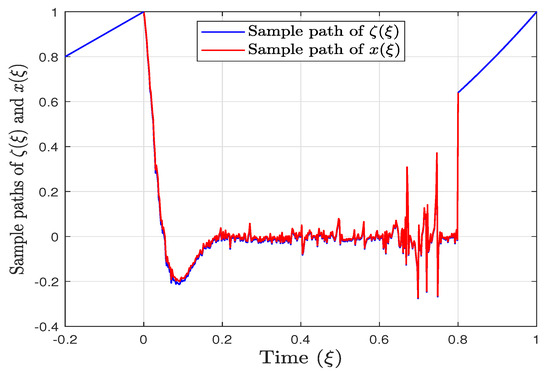
For Equation (15), we conduct a simulation based on the Euler–Maruyama scheme with a step size ${10}^{-6}$ and the chosen parameters and initial condition. Hence, in Figure 1, we give the simulation trajectory of ζ and x with the same initial condition. Moreover, we can see from Figure 1 that the solution trajectory of Equation (13) (in red) almost coincides with that of Equation (15) (in blue). It follows that the distance between $\zeta \left(\xi \right)$ and $x\left(\xi \right)$ is less than a constant, which shows that Equation (15) is $\mathcal{HU}$-stable on $\mathrm{J}$ according to Definition 3.

6. Conclusions

In this work, we explored the existence and uniqueness of neutral $\mathcal{SFDE}$s using $\mathcal{FP}$ theorems and basic notions of stochastic analysis. Additionally, we established $\mathcal{HU}$ stability under specific assumptions and conditions. Ulam’s stability is a significant concept, as it provides a bound between approximate and exact solutions, making our findings potentially valuable in the context of approximation theory for $\mathcal{SFDE}$s. Finally, we presented a relevant example to illustrate our main findings. Looking ahead, we plan to investigate the exact controllability of $\mathcal{SFDE}$s under impulsive conditions, with a particular focus on the impact of noise and memory effects.

References

- Podlubny, I. Fractional Differential Equations; Academic Press: Cambridge, MA, USA, 1999. [Google Scholar]
- Lakshmikantham, V.; Leela, S.; Devi, J.V. Theory of Fractional Dynamic Systems; Cambridge Scientific Publishers: Cambridge, UK, 2009. [Google Scholar]
- Sun, H.; Zhang, Y.; Baleanu, D.; Chen, W.; Chen, Y. A new collection of real world applications of fractional calculus in science and engineering. Commun. Nonlinear Sci. Numer. Simul. 2018, 64, 213–231. [Google Scholar] [CrossRef]
- Balachandran, K.; Park, J.Y. Controllability of fractional integrodifferential systems in Banach spaces. Nonlinear Anal. Hybrid Syst. 2009, 3, 363–367. [Google Scholar] [CrossRef]
- Miller, K.S.; Ross, B. An Introduction to the Fractional Calculus and Differential Equations; John Wiley: Hoboken, NJ, USA, 1993. [Google Scholar]
- Diethelm, K. The Analysis of Fractional Differential Equations; Lecture Notes in Mathematics; Springer: Berlin/Heidelberg, Germany, 2010. [Google Scholar]
- Zhou, Y. Basic Theory of Fractional Differential Equations; World Scientific: Singapore, 2014. [Google Scholar]
- Stirzaker, D.; Grimmett, G. Stochastic Processes and Their Applications; Springer: Berlin/Heidelberg, Germany, 2001. [Google Scholar]
- Zada, A.; Ali, W.; Farina, S. Hyers-Ulam stability of nonlinear differential equations with fractional integrable impulses. Math. Methods Appl. Sci. 2017, 40, 5502–5514. [Google Scholar] [CrossRef]
- Zada, A.; Ali, W.; Park, C. Ulam’s type stability of higher order nonlinear delay differential equations via integral inequality of Gronwal Bellman. Bihari’s type. Appl. Math. Comput. 2019, 350, 60–65. [Google Scholar]
- Zada, A.; Ali, S. Stability analysis of multi-point boundary value problem for sequential fractional differential equations with non-instantaneous impulses. Int. J. Nonlinear Sci. Numer. Simul. 2018, 19, 763–774. [Google Scholar] [CrossRef]
- Zada, A.; Shaleena, S.; Li, T. Stability analysis of higher order nonlinear differential equations in β-normed spaces. Math. Methods Appl. Sci. 2019, 42, 1151–1166. [Google Scholar] [CrossRef]
- Cui, J.; Yan, L. Existence result for fractional neutral stochastic integro-differential equations with infinite delay. J. Phys. A Math. Theor. 2011, 44, 335201. [Google Scholar] [CrossRef]
- Ahmed, M.; Zada, A.; Ahmed, J.; Mohamed, A. Analysis of stochastic weighted impulsive neutral ψ-Hilfer integro fractional differential system with delay. Math. Probl. Eng. 2022, 2022. [Google Scholar] [CrossRef]
- Hu, W.; Zhu, Q.; Karimi, H.R. Some improved Razumikhin stability criteria for impulsive stochastic delay differential systems. IEEE Trans. Autom. Control 2019, 64, 5207–5213. [Google Scholar] [CrossRef]
- Liu, K.; Feckan, M.; O’Regan, D.; Wang, J. Hyers–Ulam Stability and Existence of Solutions for Differential Equations with Caputo-Fabrizio Fractional Derivative. Mathematics 2019, 7, 333. [Google Scholar] [CrossRef]
- Wang, B.; Zhu, Q. Stability analysis of semi-Markov switched stochastic systems. Automatica 2018, 94, 72–80. [Google Scholar] [CrossRef]
- Wang, H.; Zhu, Q. Global stabilization of a class of stochastic nonlinear time-delay systems with SISS inverse dynamics. IEEE Trans. Autom. Control 2020, 65, 4448–4455. [Google Scholar] [CrossRef]
- Xie, W.; Zhu, Q. Self-triggered state-feedback control for stochastic nonlinear systems with Markovian switching. IEEE Trans. Syst. Man Cybern. 2020, 50, 3200–3209. [Google Scholar] [CrossRef]
- Zhu, Q. Stability analysis of stochastic delay differential equations with Lévy noise. Syst. Control Lett. 2018, 118, 62–68. [Google Scholar] [CrossRef]
- Zhu, Q.; Wang, H. Output feedback stabilization of stochastic feedforward systems with unknown control coefficients and unknown output function. Automatica 2018, 87, 165–175. [Google Scholar] [CrossRef]
- Dhayal, R.; Malik, M. Stability analysis of damped fractional stochastic differential systems with Poisson jumps: An successive approximation approach. Int. J. Syst. Sci. 2024, 1–13. [Google Scholar] [CrossRef]
- Hammad, H.A.; Aydi, H.; Isik, H.; De la Sen Parte, M. Existence and stability results for a coupled system of impulsive fractional differential equations with Hadamard fractional derivatives. Aims Math. 2023, 8, 6913–6941. [Google Scholar] [CrossRef]
- Khan, A.; Khan, H.; Gomez-Aguilar, J.F.; Abdeljawad, T. Existence and Hyers-Ulam stability for a nonlinear singular fractional differential equations with Mittag-Leffler kernel. Chaos Solitons Fractals 2019, 127, 422–427. [Google Scholar] [CrossRef]
- Yang, M.; Zhou, Y. Hilfer fractional stochastic evolution equations on infinite interval. Int. J. Nonlinear Sci. Numer. Simul. 2023, 24, 1841–1862. [Google Scholar] [CrossRef]
- Yang, M.; Lv, T.; Wang, Q. The averaging principle for Hilfer fractional stochastic evolution equations with Levy noise. Fractal Fract. 2023, 7, 701. [Google Scholar] [CrossRef]
- Saifullah, S.; Shahid, S.; Zada, A. Analysis of Neutral Stochastic Fractional Differential Equations Involving Riemann-Liouville Fractional Derivative with Retarded and Advanced Arguments. Qual. Theory Dyn. Syst. 2024, 23, 39. [Google Scholar] [CrossRef]
- Kilbas, A.A.; Srivastava, H.M.; Trujillo, J.J. Theory and Applications of Fractional Differential Equations. In North–Holland Mathematics Studies; Elsevier: Amsterdam, The Netherlands, 2006; p. 204. [Google Scholar]
- Umamaheswari, P.; Balachandran, K.; Annapoorani, N. Existence and stability re sults for Caputo fractional stochastic di erential equations with Levy noise. Filomat 2020, 34, 1739–1751. [Google Scholar] [CrossRef]
- Granas, A.; Dugundji, J. Fixed Point Theory; Springer: New York, NY, USA, 2003. [Google Scholar]
- Yan, B. Boundary value problems on the half-line with impulses and infinite delay. J. Math. Anal. Appl. 2001, 259, 94–114. [Google Scholar] [CrossRef]
- Deinz, H. On the behaviour of measure of noncompactness with respect to differentiation and integration of vector-valued functions. Nonlinear Anal. TMA 1983, 7, 1351–1371. [Google Scholar]
- Bellman, R. The stability of solutions of linear differential equations. Duke Math. J. 1943, 10, 643–647. [Google Scholar] [CrossRef]
- Deng, S.; Shu, X.; Mao, J. Existence and exponential stability for impulsive neutral stochastic functional differential equations driven by fBm with noncompact semigroupvia Mönch fixed point. J. Math. Anal. Appl. 2018, 467, 398–420. [Google Scholar] [CrossRef]
Disclaimer/Publisher’s Note: The statements, opinions and data contained in all publications are solely those of the individual author(s) and contributor(s) and not of MDPI and/or the editor(s). MDPI and/or the editor(s) disclaim responsibility for any injury to people or property resulting from any ideas, methods, instructions or products referred to in the content. |
© 2024 by the authors. Licensee MDPI, Basel, Switzerland. This article is an open access article distributed under the terms and conditions of the Creative Commons Attribution (CC BY) license (https://creativecommons.org/licenses/by/4.0/).