Boosted Whittaker–Henderson Graduation

Abstract

The Whittaker–Henderson (WH) graduation is a smoothing method for equally spaced one-dimensional data such as time series. It includes the Bohlmann filter, the Hodrick–Prescott (HP) filter, and the Whittaker graduation as special cases. Among them, the HP filter is the most prominent trend-cycle decomposition method for macroeconomic time series such as real gross domestic product. Recently, a modification of the HP filter, the boosted HP (bHP) filter, has been developed, and several studies have been conducted. The basic idea of the modification is to achieve more desirable smoothing by extracting long-term fluctuations remaining in the smoothing residuals. Inspired by the modification, this paper develops the boosted version of the WH graduation, which includes the bHP filter as a special case. Then, we establish its properties that are fundamental for applied work. To investigate the properties, we use a spectral decomposition of the penalty matrix of the WH graduation

1. Introduction

The Whittaker–Henderson (WH) graduation is a smoothing method for equally spaced one-dimensional data such as time series. It includes the Bohlmann (1899) [1] filter, Hodrick–Prescott (HP) filter (Hodrick and Prescott, 1997 [2]), and Whittaker (1923) [3] graduation as its special cases [4,5,6,7]. Among them, the HP filter is the most prominent trend-cycle decomposition method for macroeconomic time series such as real gross domestic product. Recently, Phillips and Shi (2021) [8] developed its modification, the boosted HP (bHP) filter. The basic idea of the modification is to achieve more desirable smoothing by extracting long-term fluctuations remaining in the smoothing residuals [8,9].

Several studies concerning the bHP filter have since emerged: (i) Knight (2021) [10] derived the penalized least squares problems corresponding to the bHP filter, (ii) Tomal (2022) [11] and Trojanek et al. (2023) [12] published empirical studies using the bHP filter, (iii) Hall and Thomson (2024) [13] provided a way to use the bHP filter as a frequency-selective filter, (iv) Mei et al. (2024) [14] and Biswas et al. (2024) [15] extended the bHP filter theoretically, (v) Yamada (2024) [9] provided a perspective of the bHP filter, (vi) Yamada (2024) [16] established the properties of the bHP filter, and (vii) Bao and Yamada (2024) [17] studied the boosted version of the Bohlmann filter.

Inspired by Phillips and Shi (2021) [8], this paper develops the boosted version of the WH graduation, the bWH graduation, which includes the bHP filter as a special case. As in the case of the bHP filter, the new filter can also recover long-term fluctuations remaining in the smoothing residuals. Then, we establish its properties, which are fundamental for applied work. To examine them, we use a spectral decomposition of the penalty matrix of the WH graduation, which is a banded symmetric matrix. This direction of research is suggested by Yamada (2024) [16], and this paper can be considered as an extension of Yamada (2024) [16]. In addition, since the boosted version of the Bohlmann filter is identical to the bWH graduation of order 1, this paper can also be considered as an extension of Bao and Yamada (2024) [17].

The organization of this paper is as follows. In Section 2, we provide some preliminary remarks, which include the spectral decomposition of the penalty matrix of the WH graduation. In Section 3, we define the bWH graduation and present the spectral representation of it. In Section 4, we establish several properties of the bWH graduation. In Section 5, we empirically illustrate the results obtained. Section 6 concludes the paper. In the Appendix A, we provide some of the proofs.

2. Preliminaries

In this section, we provide some preliminary remarks.

2.1. Data

Let $y_t$ denote the realization of a variable y at $v_t$ for $t=1,\dots ,n$, where $v_1,\dots ,v_n$ are equally spaced. In this paper, we assume that $y_t$ cannot be represented as ${\sum }_{k=0}^{p-1}{\varphi }_k{t}^k$ for $t=1,\dots ,n$, where ${\varphi }_k$ for $k=0,\dots ,p-1$ are real numbers. This is because there is no need for smoothing in this case.

2.2. Notations

Let $\mathit{y}={[y_1,\dots ,y_n]}^{\top }$, $\mathit{x}={[x_1,\dots ,x_n]}^{\top }$, $\mathit{\iota }$ be an n-dimensional column vector of ones, ${\mathbf{0}}_{r,s}$ be an $r\times s$ matrix of zeros, and ${\mathit{I}}_r$ be an $r\times r$ identity matrix. For an r-dimensional column vector $\mathit{\eta }={[{\eta }_1,\dots ,{\eta }_r]}^{\top }$, ${\parallel \mathit{\eta }\parallel }^2={\mathit{\eta }}^{\top }\mathit{\eta }={\sum }_{t=1}^r{\eta }_t^2$. For a full-column rank matrix $\mathbf{\Gamma }\in {\mathbb{R}}^{r\times s}$, the column space of $\mathbf{\Gamma }$ and its orthogonal complement are denoted by by $\mathbb{S}(\mathbf{\Gamma })$ and ${\mathbb{S}}^{\perp }(\mathbf{\Gamma })$, respectively. Let $\Delta =1-L$, where L is the lag operator such that $L{x}_t=x_{t-1}$. Accordingly, $\Delta =1-L$ is the difference operator such that $\Delta x_t=(1-L)x_t=x_t-x_{t-1}$ and ${\Delta }^2{x}_t={(1-L)}^2{x}_t=x_t-2x_{t-1}+x_{t-2}$.

2.3. Key Matrices

2.3.1. ${\mathbf{\Delta }}_{\mathit{p}}$ and ${\mathit{C}}_{\mathit{p}}$

For an n-dimensional column vector $\mathit{\zeta }={[{\zeta }_1,\dots ,{\zeta }_n]}^{\top }$, let ${\mathbf{\Delta }}_p$ be an $(n-p)\times n$ matrix such that ${\mathbf{\Delta }}_p\mathit{\zeta }={[{\Delta }^p{\zeta }_{p+1},\dots ,{\Delta }^p{\zeta }_n]}^{\top }$. Based on the binomial theorem, letting $a_h={(-1)}^{p-h}\left({\displaystyle \genfrac{}{}{0pt}{}{p}{h}}\right)$ for $h=0,1,\dots ,p$, ${(1-L)}^p$ can be expanded as follows:

$$\begin{array}{c}\hfill {(1-L)}^p={\{(-1)L+1\}}^p=\sum _{h=0}^p\left({\displaystyle \genfrac{}{}{0pt}{}{p}{h}}\right){(-1)}^{p-h}{L}^{p-h}{1}^h=\sum _{h=0}^p{a}_h{L}^{p-h}.\end{array}$$

(1)

Then, it follows that:

$$\begin{array}{cc}\hfill {\Delta }^p{x}_t& ={(1-L)}^p{x}_t=\left(\sum _{h=0}^p{a}_h{L}^{p-h}\right)x_t\hfill \\ \hfill & =a_0{x}_{t-p}+a_1{x}_{t-p+1}+\cdots +a_p{x}_t,t=p+1,\dots ,n.\hfill \end{array}$$

(2)

Accordingly, ${\mathbf{\Delta }}_p$ is an $(n-p)\times n$ Toeplitz matrix given as follows:

$$\begin{array}{c}\hfill {\mathbf{\Delta }}_p=\left[\begin{array}{cccccc}{a}_0& \cdots & a_p& 0& \cdots & 0\\ 0& \ddots & & \ddots & \ddots & ⋮\\ ⋮& \ddots & \ddots & & \ddots & 0\\ 0& \cdots & 0& a_0& \cdots & a_p\end{array}\right].\end{array}$$

(3)

Here, $a_0=-1$ if p is odd and $a_0=1$ if p is even; therefore, the rank of ${\mathbf{\Delta }}_p$ is $(n-p)$ and the nullity of ${\mathbf{\Delta }}_p$ is p. For example, ${\mathbf{\Delta }}_1\in {\mathbb{R}}^{(n-1)\times n}$ and ${\mathbf{\Delta }}_2\in {\mathbb{R}}^{(n-2)\times n}$ are given as follows, respectively:

$$\begin{array}{c}\hfill {\mathbf{\Delta }}_1=\left[\begin{array}{ccccc}-1& 1& 0& \cdots & 0\\ 0& \ddots & \ddots & \ddots & ⋮\\ ⋮& \ddots & \ddots & \ddots & 0\\ 0& \cdots & 0& -1& 1\end{array}\right],{\mathbf{\Delta }}_2=\left[\begin{array}{cccccc}1& -2& 1& 0& \cdots & 0\\ 0& \ddots & \ddots & \ddots & \ddots & ⋮\\ ⋮& \ddots & \ddots & \ddots & \ddots & 0\\ 0& \cdots & 0& 1& -2& 1\end{array}\right].\end{array}$$

Let ${\mathit{C}}_p$ be an $n\times n$-banded symmetric matrix defined as follows:

$$\begin{array}{c}\hfill {\mathit{C}}_p={\mathbf{\Delta }}_p^{\top }{\mathbf{\Delta }}_p.\end{array}$$

(4)

Then, ${\mathit{C}}_p$ is a positive semidefinite matrix whose rank is $(n-p)$. Incidentally, ${\mathit{C}}_1,\dots ,{\mathit{C}}_4$ are explicitly shown in Anderson (1971, pp. 68–69) [18]. In addition, ${\mathit{C}}_1$ is $A_2$ in Strang (1999) [19], and it is also shown in Nakatsukasa et al. (2013, p. 3233) [20].

2.3.2. ${\mathbf{\Pi }}_{\mathit{p}}$

Let

$$\begin{array}{c}\hfill {\mathbf{\Pi }}_p=[{\mathit{\tau }}_{\left(0\right)},\dots ,{\mathit{\tau }}_{(p-1)}],\end{array}$$

(5)

where ${\mathit{\tau }}_{\left(k\right)}={[1^k,2^k,\dots ,n^k]}^{\top }$ for $k=0,\dots ,p-1$. More specifically, it is a Vandermonde matrix given as follows:

$$\begin{array}{c}\hfill {\mathbf{\Pi }}_p=\left[\begin{array}{cccc}{1}^0& 1^1& \cdots & 1^{p-1}\\ 2^0& 2^1& \cdots & 2^{p-1}\\ ⋮& ⋮& & ⋮\\ n^0& n^1& \cdots & n^{p-1}\end{array}\right].\end{array}$$

(6)

Then, ${\mathbf{\Pi }}_p$ is of full column rank, and the first column of ${\mathbf{\Pi }}_p$, ${\mathit{\tau }}_{\left(0\right)}$, is equal to $\mathit{\iota }$. In addition, by assumption, $\mathit{y}\notin \mathbb{S}\left({\mathbf{\Pi }}_p\right)$.

Let

$$\begin{array}{c}\hfill {\widehat{\mathit{\tau }}}_p={\mathbf{\Pi }}_p{\widehat{\mathit{\beta }}}_p,\end{array}$$

(7)

where ${\widehat{\mathit{\beta }}}_p={\left({\mathbf{\Pi }}_p^{\top }{\mathbf{\Pi }}_p\right)}^{-1}{\mathbf{\Pi }}_p^{\top }\mathit{y}=\arg {min}_{\mathit{\beta }}{\parallel \mathit{y}-{\mathbf{\Pi }}_p\mathit{\beta }\parallel }^2$. For example, ${\widehat{\mathit{\tau }}}_1=\overline{y}{\mathit{\tau }}_{\left(0\right)}=\overline{y}\mathit{\iota }$, where $\overline{y}={\displaystyle \frac{1}{n}}{\sum }_{t=1}^n{y}_t$ and ${\widehat{\mathit{\tau }}}_2={\alpha }^{\mathrm{ba}}{\mathit{\tau }}_{\left(0\right)}+{\beta }^{\mathrm{ba}}{\mathit{\tau }}_{\left(1\right)}$, where ${\alpha }^{\mathrm{ba}}$ and ${\beta }^{\mathrm{ba}}$ are explicitly shown in Kim et al. (2009, p. 341) [21]. ${\widehat{\mathit{\tau }}}_p$ is the orthogonal projection of $\mathit{y}$ onto $\mathbb{S}\left({\mathbf{\Pi }}_p\right)$.

2.3.3. ${\mathit{D}}_{\mathit{p}}$ and ${\mathit{U}}_{\mathit{p}}$

Denote a spectral decomposition of ${\mathit{C}}_p$, which is defined by (4) as follows:

$$\begin{array}{c}\hfill {\mathit{C}}_p={\mathit{U}}_p{\mathit{D}}_p{\mathit{U}}_p^{\top },\end{array}$$

(8)

where ${\mathit{D}}_p=\mathrm{diag}(d_{p,1},\dots ,d_{p,n})$, and ${\mathit{U}}_p=[{\mathit{u}}_{p,1},\dots ,{\mathit{u}}_{p,n}]$ is an orthogonal matrix. Given that ${\mathit{C}}_p$ is a positive semidefinite matrix whose rank is $(n-p)$, we let

$$\begin{array}{c}\hfill 0=d_{p,1}=\cdots =d_{p,p}<d_{p,p+1}\le \cdots \le d_{p,n}.\end{array}$$

(9)

Here, the largest eigenvalue of ${\mathit{C}}_p$ is upper bounded by $2^{2p}$, i.e., it follows that

$$\begin{array}{c}\hfill d_{p,n}\le 2^{2p}.\end{array}$$

(10)

A proof of the last inequality in (10) is provided in Appendix A.1. Figure 1 depicts $d_{p,1},\dots ,d_{p,n}$ for $p=3$ and $n=50$. Note that if $p=3$, it follows that $d_{p,n}\le 2^{2p}=64$. We can confirm this from the figure. Since ${\mathit{C}}_p\mathit{\iota }={\mathbf{\Delta }}_p^{\top }{\mathbf{\Delta }}_p\mathit{\iota }={\mathbf{0}}_{n,1}$, we can let $(d_{p,1},{\mathit{u}}_{p,1})=\left(0,{\displaystyle \frac{1}{\sqrt{n}}}\mathit{\iota }\right)$.

2.3.4. ${\mathit{D}}_{\mathit{p},\mathit{j}}$ and ${\mathit{U}}_{\mathit{p},\mathit{j}}$ for $\mathit{j}=\mathbf{1},\mathbf{2}$

Let ${\mathit{D}}_{p,1}=\mathrm{diag}(d_{p,1},\dots ,d_{p,p})$ and ${\mathit{D}}_{p,2}=\mathrm{diag}(d_{p,p+1},\dots ,d_{p,n})$. Accordingly, it follows that

$$\begin{array}{c}\hfill {\mathit{D}}_p=\left[\begin{array}{cc}{\mathit{D}}_{p,1}& {\mathbf{0}}_{p,n-p}\\ {\mathbf{0}}_{n-p,n}& {\mathit{D}}_{p,2}\end{array}\right],\end{array}$$

In addition, from the inequalities in (9), ${\mathit{D}}_{p,1}={\mathbf{0}}_{p,p}$, and ${\mathit{D}}_{p,2}\in {\mathbb{R}}^{(n-p)\times (n-p)}$ is a positive definite matrix. Let ${\mathit{U}}_{p,1}=[{\mathit{u}}_{p,1},\dots ,{\mathit{u}}_{p,p}]$ and ${\mathit{U}}_{p,2}=[{\mathit{u}}_{p,p+1},\dots ,{\mathit{u}}_{p,n}]$. Accordingly,

$$\begin{array}{c}\hfill {\mathit{U}}_p=[{\mathit{U}}_{p,1},{\mathit{U}}_{p,2}].\end{array}$$

2.4. Results Regarding the Key Matrices

For $k=0,\dots ,p-1$, ${\mathit{\tau }}_{\left(k\right)}$ in (5) belonging to the null space of ${\mathbf{\Delta }}_p$ in (3), it follows that

$$\begin{array}{c}\hfill {\mathbf{\Delta }}_p{\mathit{\tau }}_{\left(k\right)}={\mathbf{0}}_{n-p,1}.\end{array}$$

(11)

A proof of (11) is provided in Appendix A.2. Accordingly, we have

$$\begin{array}{c}\hfill {\mathbf{\Delta }}_p{\mathbf{\Pi }}_p=[{\mathbf{\Delta }}_p{\mathit{\tau }}_{\left(0\right)},\dots ,{\mathbf{\Delta }}_p{\mathit{\tau }}_{(p-1)}]={\mathbf{0}}_{n-p,p},\end{array}$$

from which it follows that

$$\begin{array}{c}\hfill {\mathit{C}}_p{\mathbf{\Pi }}_p={\mathbf{\Delta }}_p^{\top }{\mathbf{\Delta }}_p{\mathbf{\Pi }}_p={\mathbf{0}}_{n,p}.\end{array}$$

(12)

Thus, given that (i) the nullity of ${\mathit{C}}_p$ is p and (ii) ${\mathbf{\Pi }}_p=[{\mathit{\tau }}_{\left(0\right)},\dots ,{\mathit{\tau }}_{(p-1)}]$ is of full column rank, $\{{\mathit{\tau }}_{\left(0\right)},\dots ,{\mathit{\tau }}_{(p-1)}\}$ is a basis of the null space of ${\mathit{C}}_p$. On the other hand, from (8) and (9), it follows that

$$\begin{array}{c}\hfill {\mathit{C}}_p{\mathit{U}}_{p,1}={\mathbf{0}}_{n,p},\end{array}$$

(13)

which implies that $\{{\mathit{u}}_{p,1},\dots ,{\mathit{u}}_{p,p}\}$ is an orthonormal basis of the null space of ${\mathit{C}}_p$. Combining these results, it follows that

$$\begin{array}{c}\hfill \mathbb{S}\left({\mathbf{\Pi }}_p\right)=\mathbb{S}\left({\mathit{U}}_{p,1}\right).\end{array}$$

(14)

From (14), we obtain the following two results:

$$\begin{array}{c}{\mathit{U}}_{p,1}{\mathit{U}}_{p,1}^{\top }(={\mathit{U}}_{p,1}{\left({\mathit{U}}_{p,1}^{\top }{\mathit{U}}_{p,1}\right)}^{-1}{\mathit{U}}_{p,1}^{\top })={\mathbf{\Pi }}_p{\left({\mathbf{\Pi }}_p^{\top }{\mathbf{\Pi }}_p\right)}^{-1}{\mathbf{\Pi }}_p^{\top },\end{array}$$

(15)

$$\begin{array}{c}{\mathit{U}}_{p,2}^{\top }{\mathbf{\Pi }}_p={\mathbf{0}}_{n-p,p}.\end{array}$$

(16)

Given that ${\mathit{C}}_p={\mathbf{\Delta }}_p^{\top }{\mathbf{\Delta }}_p$ and ${\mathit{C}}_p{\mathit{u}}_{p,i}=d_{p,i}{\mathit{u}}_{p,i}$ for $i=1,\dots ,n$, we have

$$\begin{array}{c}\hfill \parallel {\mathbf{\Delta }}_p{\mathit{u}}_{p,i}{\parallel }^2={\mathit{u}}_{p,i}^{\top }{\mathit{C}}_p{\mathit{u}}_{p,i}=d_{p,i},i=1,\dots ,n.\end{array}$$

(17)

Then, from (9) and (10), it follows that

$$\begin{array}{c}\hfill 0=\parallel {\mathbf{\Delta }}_p{\mathit{u}}_{p,1}{\parallel }^2=\cdots =\parallel {\mathbf{\Delta }}_p{\mathit{u}}_{p,p}{\parallel }^2\le \parallel {\mathbf{\Delta }}_p{\mathit{u}}_{p,p+1}{\parallel }^2\le \cdots \le {\parallel {\mathbf{\Delta }}_p{\mathit{u}}_{p,n}\parallel }^2\le 2^{2p}.\end{array}$$

(18)

These indicate that with respect to ${\mathbf{\Delta }}_p$, which is defined by (3),

(i)

the degree of smoothness of ${\mathit{u}}_{p,1},\dots ,{\mathit{u}}_{p,p}$ is the highest, and

(ii)

the degree of smoothness of ${\mathit{u}}_{p,i}$ is higher than or equal to that of ${\mathit{u}}_{p,i+1}$ for $i=p,\dots ,n-1$.

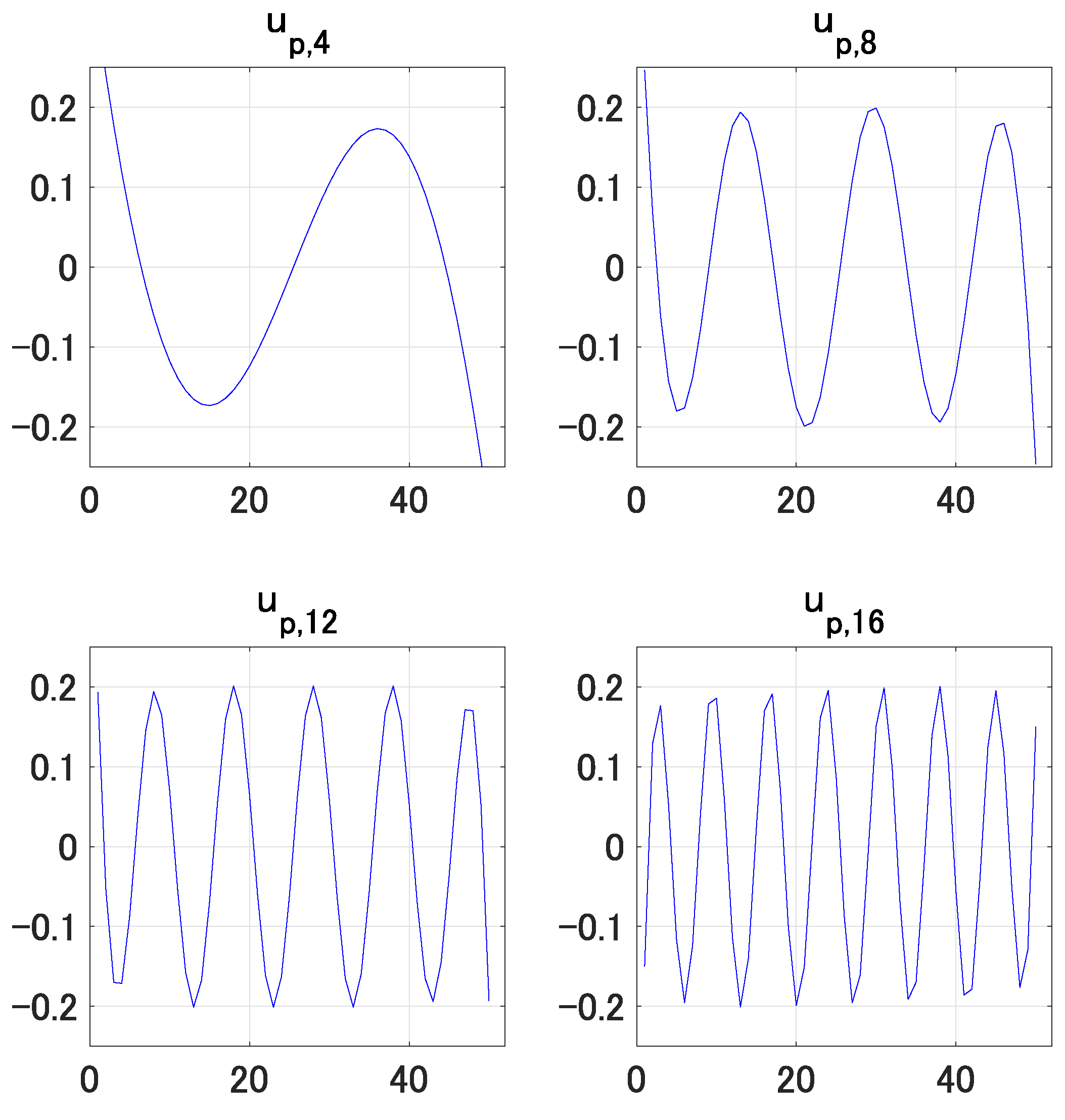
Figure 2 depicts ${\mathit{u}}_{p,4}$, ${\mathit{u}}_{p,8}$, ${\mathit{u}}_{p,12}$, ${\mathit{u}}_{p,16}$ for $p=3$ and $n=50$. This figure is consistent with (ii).

2.5. WH Graduation

The WH(p) graduation is a smoothing method given as follows:

$$\begin{array}{c}\hfill \underset{x_1,\dots ,x_n\in \mathbb{R}}{min}\sum _{t=1}^n{(y_t-x_t)}^2+{\lambda }_p\sum _{t=p+1}^n{\left({\Delta }^p{x}_t\right)}^2,\end{array}$$

(19)

where ${\lambda }_p\in (0,\infty )$ is a smoothing parameter and p is a positive integer such that $n>p$. It is a penalized least squares regression. When $p=1$, since $\Delta x_t=(1-L)x_t=x_t-x_{t-1}$, (19) is identical to the Bohlmann filter. When $p=2$, since ${\Delta }^2{x}_t=(1-2L+L^2)x_t=x_t-2x_{t-1}+x_{t-2}$, (19) is identical to the HP filter, given as follows:

$$\begin{array}{c}\hfill \underset{x_1,\dots ,x_n\in \mathbb{R}}{min}\sum _{t=1}^n{(y_t-x_t)}^2+{\lambda }_2\sum _{t=3}^n{(x_t-2x_{t-1}+x_{t-2})}^2.\end{array}$$

(20)

When $p=3$, (19) is identical to the Whittaker graduation.

The WH(p) graduation can be represented in matrix form as follows:

$$\begin{array}{c}\hfill \underset{\mathit{x}}{min}{f}_p\left(\mathit{x}\right)={\parallel \mathit{y}-\mathit{x}\parallel }^2+{\lambda }_p{\mathit{x}}^{\top }{\mathit{C}}_p\mathit{x}.\end{array}$$

(21)

Then, ${\mathit{C}}_p$, which is defined by (4), is the penalty matrix of the WH graduation. Denoting the solution to the minimization problem in (21) by ${\widehat{\mathit{x}}}_p$, it follows that

$$\begin{array}{c}\hfill {\widehat{\mathit{x}}}_p={\mathit{A}}_p\mathit{y},\end{array}$$

(22)

where

$$\begin{array}{c}\hfill {\mathit{A}}_p={({\mathit{I}}_n+{\lambda }_p{\mathit{C}}_p)}^{-1}.\end{array}$$

(23)

${\mathit{A}}_p$ is referred to as the smoother matrix of the WH(p) graduation.

2.6. Spectral Representation of WH Graduation

Given the spectral decomposition of ${\mathit{C}}_p$ in (8), ${\mathit{A}}_p$, which is the smoother matrix of the WH(p) graduation, can be spectrally decomposed as follows:

$$\begin{array}{c}\hfill {\mathit{A}}_p={({\mathit{I}}_n+{\lambda }_p{\mathit{C}}_p)}^{-1}={\mathit{U}}_p{({\mathit{I}}_n+{\lambda }_p{\mathit{D}}_p)}^{-1}{\mathit{U}}_p^{\top }={\mathit{U}}_p{\mathit{B}}_p{\mathit{U}}_p^{\top },\end{array}$$

(24)

where ${\mathit{B}}_p={({\mathit{I}}_n+{\lambda }_p{\mathit{D}}_p)}^{-1}$. Let ${\mathit{B}}_p=\mathrm{diag}(b_{p,1},\dots ,b_{p,n})$. Then, given that

$$\begin{array}{c}\hfill b_{p,i}={(1+{\lambda }_p{d}_{p,i})}^{-1},i=1,\dots ,n,\end{array}$$

(25)

from the inequalities in (9), it follows that

$$\begin{array}{c}\hfill 1=b_{p,1}=\cdots =b_{p,p}>b_{p,p+1}\ge \cdots \ge b_{p,n}>0.\end{array}$$

(26)

3. Boosted WH Graduation

3.1. Boosted WH Graduation

We define the boosted WH graduation of order p, bWH(p) graduation for short, as follows:

$$\begin{array}{c}\hfill {\widehat{\mathit{x}}}_p^{\left(m\right)}={\mathit{A}}_p^{\left(m\right)}\mathit{y},\end{array}$$

(27)

where

$$\begin{array}{c}\hfill {\mathit{A}}_p^{\left(m\right)}={\mathit{I}}_n-{({\mathit{I}}_n-{\mathit{A}}_p)}^m.\end{array}$$

(28)

We refer to ${\mathit{A}}_p^{\left(m\right)}$ as the smoother matrix of the bWH(p) graduation.

The bWH(p) graduation is related to the existing filters as follows. In our notation, the boosted HP filter developed by Phillips and Shi (2021) [8] is represented as follows:

$$\begin{array}{c}\hfill {\widehat{\mathit{x}}}_2^{\left(m\right)}={\mathit{A}}_2^{\left(m\right)}\mathit{y}.\end{array}$$

(29)

Thus, bWH(p) graduation is a generalization of the bHP filter. In addition, since

$$\begin{array}{c}\hfill {\mathit{A}}_p^{\left(1\right)}={\mathit{I}}_n-({\mathit{I}}_n-{\mathit{A}}_p)={\mathit{A}}_p,\end{array}$$

(30)

the bWH(p) graduation is also a generalization of the WH(p) graduation. Moreover, the bWH(1) graduation was dealt with in Bao and Yamada (2024) [17]. Finally, Hall and Thompson (2024) [13] refer to ${\widehat{\mathit{x}}}_2^{\left(2\right)}$ as twicing.

We illustrate how boosting brings a gain. Given that ${\mathit{A}}_p^{\left(2\right)}={\mathit{I}}_n-{({\mathit{I}}_n-{\mathit{A}}_p)}^2={\mathit{I}}_n-{\mathit{I}}_n+2{\mathit{A}}_p-{\mathit{A}}_p^2={\mathit{A}}_p+{\mathit{A}}_p({\mathit{I}}_n-{\mathit{A}}_p)$, it follows that

$$\begin{array}{c}\hfill {\widehat{\mathit{x}}}_p^{\left(2\right)}={\widehat{\mathit{x}}}_p+{\mathit{A}}_p(\mathit{y}-{\widehat{\mathit{x}}}_p).\end{array}$$

(31)

Here, ${\mathit{A}}_p(\mathit{y}-{\widehat{\mathit{x}}}_p)$ in (31) can be regarded as a gain from boosting. Given that ${\mathit{A}}_p$ is the smoother matrix of the WH graduation, ${\mathit{A}}_p(\mathit{y}-{\widehat{\mathit{x}}}_p)$ is a trend recovered from the WH graduation residuals, $\mathit{y}-{\widehat{\mathit{x}}}_p$.

MATLAB/GNU Octave, R, and Python user-defined functions for calculating ${\widehat{\mathit{x}}}_p^{\left(m\right)}$ in (27) are available from GitHub. The URL is https://github.com/HiroshiFromHiroshima/Boosted_Whittaker-Henderson_Graduation (accessed on 26 October 2024). We used MATLAB version R2018b, GNU Octave version 7.1.0, R version 4.2.3, and Python version 3.12.5 to verify these user-defined functions.

3.2. Spectral Representation of bWH Graduation

Given the spectral decomposition of ${\mathit{A}}_p$ in (24), ${\mathit{A}}_p^{\left(m\right)}$ in (28), which is the smoother matrix of the bWH(p) graduation, can be spectrally decomposed as follows:

$$\begin{array}{cc}\hfill {\mathit{A}}_p^{\left(m\right)}& ={\mathit{I}}_n-{({\mathit{I}}_n-{\mathit{A}}_p)}^m={\mathit{I}}_n-{({\mathit{I}}_n-{\mathit{U}}_p{\mathit{B}}_p{\mathit{U}}_p^{\top })}^m\hfill \\ \hfill & ={\mathit{U}}_p\left\{{\mathit{I}}_n-{({\mathit{I}}_n-{\mathit{B}}_p)}^m\right\}{\mathit{U}}_p^{\top }={\mathit{U}}_p{\mathit{B}}_p^{\left(m\right)}{\mathit{U}}_p^{\top },\hfill \end{array}$$

(32)

where

$$\begin{array}{c}\hfill {\mathit{B}}_p^{\left(m\right)}={\mathit{I}}_n-{({\mathit{I}}_n-{\mathit{B}}_p)}^m.\end{array}$$

(33)

From (32), we have some useful results.

• Given that ${\mathit{B}}_p^{\left(m\right)}$ is a diagonal matrix, from (32), it follows that

  $$\begin{array}{c}\hfill {\left({\mathit{A}}_p^{\left(m\right)}\right)}^{\top }={\left({\mathit{U}}_p{\mathit{B}}_p^{\left(m\right)}{\mathit{U}}_p^{\top }\right)}^{\top }={\mathit{U}}_p{\mathit{B}}_p^{\left(m\right)}{\mathit{U}}_p^{\top }={\mathit{A}}_p^{\left(m\right)}.\end{array}$$

  (34)
  That is, ${\mathit{A}}_p^{\left(m\right)}$ is a symmetric matrix.
• Let ${\mathit{B}}_p^{\left(m\right)}=\mathrm{diag}(b_{p,1}^{\left(m\right)},\dots ,b_{p,n}^{\left(m\right)})$. Then, it follows that

  $$\begin{array}{c}\hfill b_{p,i}^{\left(m\right)}=1-{(1-b_{p,i})}^m=1-{\left({\displaystyle \frac{{\lambda }_p{d}_{p,i}}{1+{\lambda }_p{d}_{p,i}}}\right)}^m,i=1,\dots ,n.\end{array}$$

  (35)
  Thus, it follows from (26) that

  $$\begin{array}{c}\hfill 1=b_{p,1}^{\left(m\right)}=\cdots =b_{p,p}^{\left(m\right)}>b_{p,p+1}^{\left(m\right)}\ge \cdots \ge b_{p,n}^{\left(m\right)}>0.\end{array}$$

  (36)
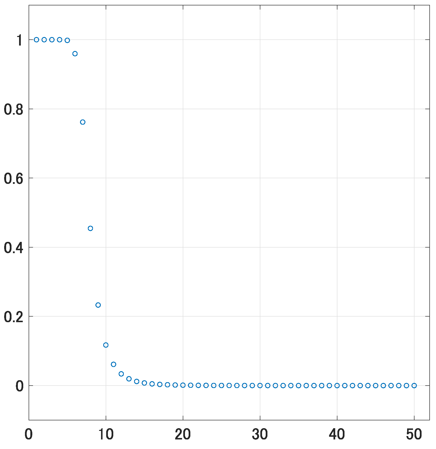
  Figure 3 depicts $b_{p,1}^{\left(m\right)},\dots ,b_{p,n}^{\left(m\right)}$ for $p=3$, $n=50$, $m=2$, and ${\lambda }_p=1000$. It illustrates the inequalities in (36).
  Then, given that ${\mathit{A}}_p^{\left(m\right)}$ is a symmetric matrix whose eigenvalues, $b_{p,i}^{\left(m\right)}$ for $i=1,\dots ,n$, are all positive, ${\mathit{A}}_p^{\left(m\right)}$ is a positive definite matrix.
• Let ${\mathit{B}}_{p,1}^{\left(m\right)}=\mathrm{diag}(b_{p,1}^{\left(m\right)},\dots ,b_{p,p}^{\left(m\right)})$ and ${\mathit{B}}_{p,2}^{\left(m\right)}=\mathrm{diag}(b_{p,p+1}^{\left(m\right)},\dots ,b_{p,n}^{\left(m\right)})$. Then, given that ${\mathit{B}}_{p,1}^{\left(m\right)}={\mathit{I}}_p$, the spectral decomposition of ${\mathit{A}}_p^{\left(m\right)}$ in (32) becomes

  $$\begin{array}{c}\hfill {\mathit{A}}_p^{\left(m\right)}={\mathit{U}}_{p,1}{\mathit{U}}_{p,1}^{\top }+{\mathit{U}}_{p,2}{\mathit{B}}_{p,2}^{\left(m\right)}{\mathit{U}}_{p,2}^{\top }.\end{array}$$

  (37)
  Moreover, from (15), ${\mathit{A}}_p^{\left(m\right)}$ can be represented as follows:

  $$\begin{array}{c}\hfill {\mathit{A}}_p^{\left(m\right)}={\mathbf{\Pi }}_p{\left({\mathbf{\Pi }}_p^{\top }{\mathbf{\Pi }}_p\right)}^{-1}{\mathbf{\Pi }}_p^{\top }+{\mathit{U}}_{p,2}{\mathit{B}}_{p,2}^{\left(m\right)}{\mathit{U}}_{p,2}^{\top }.\end{array}$$

  (38)
• Given (16), postmultiplying (37) by ${\mathbf{\Pi }}_p$ yields the following:

  $$\begin{array}{c}\hfill {\mathit{A}}_p^{\left(m\right)}{\mathbf{\Pi }}_p={\mathbf{\Pi }}_p.\end{array}$$

  (39)

Let us summarize the above results.

Lemma 1.

The smoother matrix of the bWH graduation, ${\mathit{A}}_p^{\left(m\right)}$, has the following properties.

(i) 

${\mathit{A}}_p^{\left(m\right)}$ is a symmetric matrix. Moreover, it is a positive definite matrix whose eigenvalues satisfy (36).

(ii) 

${\mathit{A}}_p^{\left(m\right)}$ can be represented as in (38).

(iii) 

${\mathit{A}}_p^{\left(m\right)}$ is a matrix such that ${\mathit{A}}_p^{\left(m\right)}{\mathbf{\Pi }}_p={\mathbf{\Pi }}_p$.

Postmultiplying (38) by $\mathit{y}$, we immediately obtain the following result.

Lemma 2.

${\widehat{\mathit{x}}}_p^{\left(m\right)}$ in (27) can be spectrally represented as

$$\begin{array}{c}\hfill {\widehat{\mathit{x}}}_p^{\left(m\right)}={\widehat{\mathit{\tau }}}_p+b_{p,p+1}^{\left(m\right)}{z}_{p,p+1}{\mathit{u}}_{p,p+1}+\cdots +b_{p,n}^{\left(m\right)}{z}_{p,n}{\mathit{u}}_{p,n},\end{array}$$

(40)

where $z_{p,i}={\mathit{u}}_{p,i}^{\top }\mathit{y}$ for $i=p+1,\dots ,n$ and ${\widehat{\mathit{\tau }}}_p\in {\mathbb{S}}^{\perp }\left({\mathit{U}}_{p,2}\right)$ is the orthogonal projection of $\mathit{y}$ onto $\mathbb{S}\left({\mathbf{\Pi }}_p\right)$.

Remark 1.

Given the inequalities in (18) and (36), the spectral representation of ${\widehat{\mathit{x}}}_p^{\left(m\right)}$ in Lemma 2 shows how smoothing is performed. See also Figure 3, which illustrates (36).

4. Properties of the bWH Graduation

In this section, we establish several properties of the bWH graduation.

For this purpose, we will introduce some notations. The t-th entry of ${\widehat{\mathit{x}}}_p^{\left(m\right)}$ in (27) is denoted by ${\widehat{x}}_{p,t}^{\left(m\right)}$ for $t=1,\dots ,n$, and the $(i,j)$-th entry of ${\mathit{A}}_p^{\left(m\right)}$ in (28) is denoted by $a_{p,i,j}^{\left(m\right)}$ for $i,j=1,\dots ,n$. Let

$$\begin{array}{c}\hfill {\mathit{C}}_p^{\left(m\right)}={\displaystyle \frac{1}{{\lambda }_p}}\left\{{\left({\mathit{A}}_p^{\left(m\right)}\right)}^{-1}-{\mathit{I}}_n\right\}.\end{array}$$

(41)

Here, we note that ${\mathit{C}}_p^{\left(m\right)}$ in (41) can be defined because ${\mathit{A}}_p^{\left(m\right)}$ is a positive definite matrix from Lemma 1(i). In addition, let

$$\begin{array}{c}\hfill {\mathit{D}}_p^{\left(m\right)}={\displaystyle \frac{1}{{\lambda }_p}}\left\{{\left({\mathit{B}}_p^{\left(m\right)}\right)}^{-1}-{\mathit{I}}_n\right\}.\end{array}$$

(42)

Here, ${\left({\mathit{B}}_p^{\left(m\right)}\right)}^{-1}$ in (42) is a diagonal matrix whose diagonal entries are all positive (See the inequalities in (36)).

Proposition 1.

The bWH graduation has the following properties.

(i) 

(a) The average of the entries of ${\widehat{\mathit{x}}}_p^{\left(m\right)}$ in (27) is equal to that of $\mathit{y}$. That is, it follows that

$$\begin{array}{c}\hfill {\displaystyle \frac{1}{n}}\sum _{t=1}^n{\widehat{x}}_{p,t}^{\left(m\right)}={\displaystyle \frac{1}{n}}\sum _{t=1}^n{y}_t.\end{array}$$

(43)

(b) The bWH graduation residuals, $\mathit{y}-{\widehat{\mathit{x}}}_p^{\left(m\right)}$, sum to zero. That is, it follows that

$$\begin{array}{c}\hfill \sum _{t=1}^n(y_t-{\widehat{x}}_{p,t}^{\left(m\right)})=0.\end{array}$$

(44)

(ii) 

The result in (i)(a) can be generalized as follows.

$$\begin{array}{c}\hfill {\displaystyle \frac{1}{n}}\sum _{t=1}^n{t}^k{\widehat{x}}_{p,t}^{\left(m\right)}={\displaystyle \frac{1}{n}}\sum _{t=1}^n{t}^k{y}_t,k=0,\dots ,p-1.\end{array}$$

(45)

(iii) 

Each row of the smoother matrix ${\mathit{A}}_p^{\left(m\right)}$ in (28) sums to unity. That is, it follows that

$$\begin{array}{c}\hfill a_{p,i,1}^{\left(m\right)}+\cdots +a_{p,i,n}^{\left(m\right)}=1,i=1,\dots ,n.\end{array}$$

(46)

(iv) 

${\widehat{\mathit{\tau }}}_p$ in (7) satisfies

$$\begin{array}{c}\hfill {\mathit{A}}_p^{\left(m\right)}{\widehat{\mathit{\tau }}}_p={\widehat{\mathit{\tau }}}_p.\end{array}$$

(47)

Accordingly, ${\widehat{\mathit{x}}}_p^{\left(m\right)}$ in (27) can be represented by ${\widehat{\mathit{\tau }}}_p$ as follows:

$$\begin{array}{c}\hfill {\widehat{\mathit{x}}}_p^{\left(m\right)}={\widehat{\mathit{\tau }}}_p+{\mathit{A}}_p^{\left(m\right)}(\mathit{y}-{\widehat{\mathit{\tau }}}_p).\end{array}$$

(48)

(v) 

When n and m are fixed, as ${\lambda }_p\to \infty$, ${\widehat{\mathit{x}}}_p^{\left(m\right)}\to {\widehat{\mathit{\tau }}}_p$.

(vi) 

When n and m are fixed, as ${\lambda }_p\to 0$, ${\widehat{\mathit{x}}}_p^{\left(m\right)}\to \mathit{y}$.

(vii) 

When n and ${\lambda }_p$ are fixed, as $m\to \infty$, ${\widehat{\mathit{x}}}_p^{\left(m\right)}\to \mathit{y}$.

(viii) 

When n, m, and ${\lambda }_p$ are fixed, as $h\to \infty$, ${\left({\mathit{A}}_p^{\left(m\right)}\right)}^h\mathit{y}\to {\widehat{\mathit{\tau }}}_p$.

(ix) 

${\widehat{\mathit{x}}}_p^{\left(m\right)}$ in (7) can be considered as the solution of a penalized least squares problem. More specifically, it follows that

$$\begin{array}{cc}\hfill {\widehat{\mathit{x}}}_p^{\left(m\right)}& =\arg \underset{\mathit{x}}{min}{f}_p^{\left(m\right)}\left(\mathit{x}\right)={\parallel \mathit{y}-\mathit{x}\parallel }^2+{\lambda }_p{\mathit{x}}^{\top }{\mathit{C}}_p^{\left(m\right)}\mathit{x}\hfill \\ \hfill & ={({\mathit{I}}_n+{\lambda }_p{\mathit{C}}_p^{\left(m\right)})}^{-1}\mathit{y}.\hfill \end{array}$$

(49)

(x) 

${\widehat{\mathit{x}}}_p^{\left(m\right)}$ in (7) can be represented by

$$\begin{array}{c}\hfill {\widehat{\mathit{x}}}_p^{\left(m\right)}={\mathit{U}}_p{\widehat{\mathit{\theta }}}_p^{\left(m\right)},\end{array}$$

(50)

where ${\mathit{U}}_p$ is an $n\times n$ orthogonal matrix in (8) and

$$\begin{array}{cc}\hfill {\widehat{\mathit{\theta }}}_p^{\left(m\right)}& =\arg \underset{\mathit{\theta }}{min}{g}_p^{\left(m\right)}\left(\mathit{\theta }\right)={\parallel \mathit{y}-{\mathit{U}}_p\mathit{\theta }\parallel }^2+{\lambda }_p{\mathit{\theta }}^{\top }{\mathit{D}}_p^{\left(m\right)}\mathit{\theta }\hfill \\ \hfill & ={({\mathit{I}}_n+{\lambda }_p{\mathit{D}}_p^{\left(m\right)})}^{-1}{\mathit{U}}_p^{\top }\mathit{y}.\hfill \end{array}$$

(51)

Here, ${\mathit{D}}_p^{\left(m\right)}$ is a diagonal matrix such that its first p diagonal entries are zeros; therefore, the first p entries of $\mathit{\theta }$ are not penalized.

(xi) 

The penalty matrices ${\mathit{C}}_p^{\left(m\right)}$ in (49) and ${\mathit{D}}_p^{\left(m\right)}$ in (51) are similar; therefore, they have the same eigenvalues. Furthermore, ${\mathit{C}}_p^{\left(m\right)}$ is a non-negative definite matrix whose null space is identical to $\mathbb{S}\left({\mathbf{\Pi }}_p\right)$.

Proof. 

The proofs of (i) to (xi) are, in turn, as follows.

(i)

$\mathit{\iota }$ is one of the columns of ${\mathbf{\Pi }}_p$ in (6). Then, its orthogonal projection onto $\mathbb{S}\left({\mathbf{\Pi }}_p\right)$ is itself; i.e., it follows that ${\mathbf{\Pi }}_p{\left({\mathbf{\Pi }}_p^{\top }{\mathbf{\Pi }}_p\right)}^{-1}{\mathbf{\Pi }}_p^{\top }\mathit{\iota }=\mathit{\iota }$. In addition, from (16), it follows that ${\mathit{\iota }}^{\top }{\mathit{u}}_{p,i}=0$ for $i=p+1,\dots ,n$. Accordingly, pre-multiplying (40) by ${\mathit{\iota }}^{\top }$ yields

$$\begin{array}{c}\hfill {\mathit{\iota }}^{\top }{\widehat{\mathit{x}}}_p^{\left(m\right)}={\mathit{\iota }}^{\top }{\mathbf{\Pi }}_p{\left({\mathbf{\Pi }}_p^{\top }{\mathbf{\Pi }}_p\right)}^{-1}{\mathbf{\Pi }}_p^{\top }\mathit{y}={\mathit{\iota }}^{\top }\mathit{y},\end{array}$$

(52)

which implies that the average of the entries of ${\widehat{\mathit{x}}}_p^{\left(m\right)}$ equals that of $\mathit{y}$. In addition, from (52), it immediately follows that

$$\begin{array}{c}\hfill {\mathit{\iota }}^{\top }(\mathit{y}-{\widehat{\mathit{x}}}_p^{\left(m\right)})=0.\end{array}$$

Thus, the bWH(p) graduation trend residuals sum to zero.

(ii)

${\mathit{\tau }}_{\left(k\right)}$ is one of the columns of ${\mathbf{\Pi }}_p$ in (6). Then, it follows that ${\mathbf{\Pi }}_p{\left({\mathbf{\Pi }}_p^{\top }{\mathbf{\Pi }}_p\right)}^{-1}{\mathbf{\Pi }}_p^{\top }{\mathit{\tau }}_{\left(k\right)}={\mathit{\tau }}_{\left(k\right)}$ for $k=0,\dots ,p-1$. In addition, from (16), it follows that ${\mathit{\tau }}_{\left(k\right)}^{\top }{\mathit{u}}_{p,i}=0$ for $k=0,\dots ,p-1$ and $i=p+1,\dots ,n$. Accordingly, pre-multiplying (40) by ${\mathit{\tau }}_{\left(k\right)}^{\top }$ yields

$$\begin{array}{c}\hfill {\mathit{\tau }}_{\left(k\right)}^{\top }{\widehat{\mathit{x}}}_p^{\left(m\right)}={\mathit{\tau }}_{\left(k\right)}^{\top }{\mathbf{\Pi }}_p{\left({\mathbf{\Pi }}_p^{\top }{\mathbf{\Pi }}_p\right)}^{-1}{\mathbf{\Pi }}_p^{\top }\mathit{y}={\mathit{\tau }}_{\left(k\right)}^{\top }\mathit{y},\end{array}$$

from which we have (45).

(iii)

Given that $\mathit{\iota }$ is one of the columns of ${\mathbf{\Pi }}_p$ in (6), it follows from (39) that

$$\begin{array}{c}\hfill {\mathit{A}}_p^{\left(m\right)}\mathit{\iota }=\mathit{\iota }.\end{array}$$

Thus, each row of the smoother matrix ${\mathit{A}}_p^{\left(m\right)}$ sums to unity.

(iv)

Again from (39), regarding ${\widehat{\mathit{\tau }}}_p$ in (7), it follows that

$$\begin{array}{c}\hfill {\mathit{A}}_p^{\left(m\right)}{\widehat{\mathit{\tau }}}_p={\mathit{A}}_p^{\left(m\right)}{\mathbf{\Pi }}_p{\left({\mathbf{\Pi }}_p^{\top }{\mathbf{\Pi }}_p\right)}^{-1}{\mathbf{\Pi }}_p^{\top }\mathit{y}={\mathbf{\Pi }}_p{\left({\mathbf{\Pi }}_p^{\top }{\mathbf{\Pi }}_p\right)}^{-1}{\mathbf{\Pi }}_p^{\top }\mathit{y}={\widehat{\mathit{\tau }}}_p,\end{array}$$

from which we immediately obtain

$$\begin{array}{c}\hfill {\widehat{\mathit{x}}}_p^{\left(m\right)}={\widehat{\mathit{\tau }}}_p+{\mathit{A}}_p^{\left(m\right)}(\mathit{y}-{\widehat{\mathit{\tau }}}_p).\end{array}$$

(v)

From (35), it follows that

$$\begin{array}{c}\hfill b_{p,i}^{\left(m\right)}=1-{\left({\displaystyle \frac{{\lambda }_p{d}_{p,i}}{1+{\lambda }_p{d}_{p,i}}}\right)}^m\to 0,(n,m:\mathrm{fixed},{\lambda }_p\to \infty )\end{array}$$

for $i=p+1,\dots ,n$. Accordingly, it follows from Lemma 2 that

$$\begin{array}{cc}\hfill {\widehat{\mathit{x}}}_p^{\left(m\right)}& ={\widehat{\mathit{\tau }}}_p+b_{p,p+1}^{\left(m\right)}{z}_{p,p+1}{\mathit{u}}_{p,p+1}+\cdots +b_{p,n}^{\left(m\right)}{z}_{p,n}{\mathit{u}}_{p,n}\hfill \\ \hfill & \to {\widehat{\mathit{\tau }}}_p,(n,m:\mathrm{fixed},{\lambda }_p\to \infty ).\hfill \end{array}$$

(vi)

From (35) and (36), it follows that $b_{p,1}^{\left(m\right)}=\cdots =b_{p,p}^{\left(m\right)}=1$ and

$$\begin{array}{c}\hfill b_{p,i}^{\left(m\right)}=1-{\left({\displaystyle \frac{{\lambda }_p{d}_{p,i}}{1+{\lambda }_p{d}_{p,i}}}\right)}^m\to 1,(n,m:\mathrm{fixed},{\lambda }_p\to 0)\end{array}$$

for $i=p+1,\dots ,n$. Accordingly, it follows from (32) that

$$\begin{array}{c}\hfill {\mathit{A}}_p^{\left(m\right)}={\mathit{U}}_p{\mathit{B}}_p^{\left(m\right)}{\mathit{U}}_p^{\top }\to {\mathit{U}}_p{\mathit{U}}_p^{\top }={\mathit{I}}_n,(n,m:\mathrm{fixed},{\lambda }_p\to 0).\end{array}$$

Therefore, we have

$$\begin{array}{c}\hfill {\widehat{\mathit{x}}}_p^{\left(m\right)}={\mathit{A}}_p^{\left(m\right)}\mathit{y}\to \mathit{y},(n,m:\mathrm{fixed},{\lambda }_p\to 0).\end{array}$$

(vii)

From (35) and (36), it follows that $b_{p,1}^{\left(m\right)}=\cdots =b_{p,p}^{\left(m\right)}=1$ and

$$\begin{array}{c}\hfill b_{p,i}^{\left(m\right)}=1-{\left({\displaystyle \frac{{\lambda }_p{d}_{p,i}}{1+{\lambda }_p{d}_{p,i}}}\right)}^m\to 1,(n,{\lambda }_p:\mathrm{fixed},m\to \infty )\end{array}$$

for $i=p+1,\dots ,n$. Accordingly, it follows from (32) that

$$\begin{array}{c}\hfill {\mathit{A}}_p^{\left(m\right)}={\mathit{U}}_p{\mathit{B}}_p^{\left(m\right)}{\mathit{U}}_p^{\top }\to {\mathit{U}}_p{\mathit{U}}_p^{\top }={\mathit{I}}_n,(n,{\lambda }_p:\mathrm{fixed},m\to \infty ).\end{array}$$

Therefore, we have

$$\begin{array}{c}\hfill {\widehat{\mathit{x}}}_p^{\left(m\right)}={\mathit{A}}_p^{\left(m\right)}\mathit{y}\to \mathit{y},(n,{\lambda }_p:\mathrm{fixed},m\to \infty ).\end{array}$$

(viii)

From (32) and (36), it follows that

$$\begin{array}{c}\hfill {\left({\mathit{A}}_p^{\left(m\right)}\right)}^h={\mathit{U}}_p{\left({\mathit{B}}_p^{\left(m\right)}\right)}^h{\mathit{U}}_p^{\top }\to {\mathit{U}}_{p,1}{\mathit{U}}_{p,1}^{\top },(n,m,{\lambda }_p:\mathrm{fixed},h\to \infty ).\end{array}$$

Accordingly, it follows from (15) that

$$\begin{array}{c}\hfill {\left({\mathit{A}}_p^{\left(m\right)}\right)}^h\mathit{y}={\mathit{U}}_p{\left({\mathit{B}}_p^{\left(m\right)}\right)}^h{\mathit{U}}_p^{\top }\mathit{y}\to {\mathit{U}}_{p,1}{\mathit{U}}_{p,1}^{\top }\mathit{y}={\widehat{\mathit{\tau }}}_p,(n,m,{\lambda }_p:\mathrm{fixed},h\to \infty ).\end{array}$$

(ix)

From the definition of ${\mathit{C}}_p^{\left(m\right)}$ given by (41), it immediately follows that ${\mathit{A}}_p^{\left(m\right)}={({\mathit{I}}_n+{\lambda }_p{\mathit{C}}_p^{\left(m\right)})}^{-1}$. Accordingly, we have

$$\begin{array}{cc}\hfill {\widehat{\mathit{x}}}_p^{\left(m\right)}& ={\mathit{A}}_p^{\left(m\right)}\mathit{y}={({\mathit{I}}_n+{\lambda }_p{\mathit{C}}_p^{\left(m\right)})}^{-1}\mathit{y}\hfill \\ \hfill & =\arg \underset{\mathit{x}}{min}{f}_p^{\left(m\right)}\left(\mathit{x}\right)={\parallel \mathit{y}-\mathit{x}\parallel }^2+{\lambda }_p{\mathit{x}}^{\top }{\mathit{C}}_p^{\left(m\right)}\mathit{x}.\hfill \end{array}$$

(x)

Based on the spectral decomposition of ${\mathit{A}}_p^{\left(m\right)}$ in (32), i.e., ${\mathit{A}}_p^{\left(m\right)}={\mathit{U}}_p{\mathit{B}}_p^{\left(m\right)}{\mathit{U}}_p^{\top }$, ${\mathit{C}}_p^{\left(m\right)}$ in (41) can be decomposed as follows:

$$\begin{array}{c}\hfill {\mathit{C}}_p^{\left(m\right)}={\displaystyle \frac{1}{{\lambda }_p}}\left\{{\mathit{U}}_p{\left({\mathit{B}}_p^{\left(m\right)}\right)}^{-1}{\mathit{U}}_p^{\top }-{\mathit{I}}_n\right\}={\mathit{U}}_p{\mathit{D}}_p^{\left(m\right)}{\mathit{U}}_p^{\top },\end{array}$$

(53)

by which we have

$$\begin{array}{cc}\hfill {\mathit{U}}_p{\widehat{\mathit{\theta }}}_p^{\left(m\right)}& ={\mathit{U}}_p{({\mathit{I}}_n+{\lambda }_p{\mathit{D}}_p^{\left(m\right)})}^{-1}{\mathit{U}}_p^{\top }\mathit{y}={({\mathit{I}}_n+{\lambda }_p{\mathit{U}}_p{\mathit{D}}_p^{\left(m\right)}{\mathit{U}}_p^{\top })}^{-1}\mathit{y}\hfill \\ \hfill & ={({\mathit{I}}_n+{\lambda }_p{\mathit{C}}_p^{\left(m\right)})}^{-1}\mathit{y}={\mathit{A}}_p^{\left(m\right)}\mathit{y}={\widehat{\mathit{x}}}_p^{\left(m\right)}.\hfill \end{array}$$

Let

$$\begin{array}{c}\hfill d_{p,i}^{\left(m\right)}={\displaystyle \frac{1}{{\lambda }_p}}\left({\displaystyle \frac{1}{b_{p,i}^{\left(m\right)}}}-1\right),i=1,\dots ,n.\end{array}$$

(54)

Then, ${\mathit{D}}_p^{\left(m\right)}=\mathrm{diag}(d_{p,1}^{\left(m\right)},\dots ,d_{p,n}^{\left(m\right)})$, and from the inequalities given in (36), it follows that

$$\begin{array}{c}\hfill 0=d_{p,1}^{\left(m\right)}=\cdots =d_{p,p}^{\left(m\right)}<d_{p,p+1}^{\left(m\right)}\le \cdots \le d_{p,n}^{\left(m\right)}.\end{array}$$

(55)

(xi)

Given that ${\mathit{U}}_p$ in (8) is an orthogonal matrix, from (53), ${\mathit{C}}_p^{\left(m\right)}$ is similar to ${\mathit{D}}_p^{\left(m\right)}$, and they have the same eigenvalues. Then, based on (55), ${\mathit{C}}_p^{\left(m\right)}$ is a non-negative definite matrix such that its nullity is p. Based on Lemma 1(i) and (39), ${\mathit{A}}_p^{\left(m\right)}$ is a positive definite matrix such that ${\mathit{A}}_p^{\left(m\right)}{\mathbf{\Pi }}_p={\mathbf{\Pi }}_p$. Then, it follows that

$$\begin{array}{c}\hfill {\left({\mathit{A}}_p^{\left(m\right)}\right)}^{-1}{\mathbf{\Pi }}_p={\mathbf{\Pi }}_p,\end{array}$$

from which we have

$$\begin{array}{c}\hfill {\mathit{C}}_p^{\left(m\right)}{\mathbf{\Pi }}_p={\displaystyle \frac{1}{{\lambda }_p}}\left\{{\left({\mathit{A}}_p^{\left(m\right)}\right)}^{-1}-{\mathit{I}}_n\right\}{\mathbf{\Pi }}_p={\displaystyle \frac{1}{{\lambda }_p}}({\mathbf{\Pi }}_p-{\mathbf{\Pi }}_p)={\mathbf{0}}_{n,p}.\end{array}$$

(56)

Thus, ${\mathit{\tau }}_{\left(0\right)},\dots ,{\mathit{\tau }}_{(p-1)}$ belong to the null space of ${\mathit{C}}_p^{\left(m\right)}$.

□

Remark 2.

Regarding Proposition 1, we make several remarks.

1. 

Some of the results in Proposition 1 are generalizations of those in Yamada (2020, Proposition 2.2) [22], which documents several properties of the HP filter. For example, Proposition 1(i) is a generalization of Yamada (2020, Proposition 2.2(iii)(a)) [22].

2. 

Since ${\mathit{A}}_p^{\left(m\right)}$ is symmetric, from ${\mathit{A}}_p^{\left(m\right)}\mathit{\iota }=\mathit{\iota }$, it follows that ${\mathit{\iota }}^{\top }{\mathit{A}}_p^{\left(m\right)}={\mathit{\iota }}^{\top }$, from which we have

$$\begin{array}{c}\hfill {\mathit{\iota }}^{\top }{\widehat{\mathit{x}}}_p^{\left(m\right)}={\mathit{\iota }}^{\top }{\mathit{A}}_p^{\left(m\right)}\mathit{y}={\mathit{\iota }}^{\top }\mathit{y}.\end{array}$$

This is another proof of Proposition 1(i)(a).

3. 

${\sum }_{t=1}^n{t}^k{\widehat{x}}_{p,t}^{\left(m\right)}={\sum }_{t=1}^n{t}^k{y}_t$ for $k=0,\dots ,p-1$ in Proposition 1(ii) is a generalization of ${\sum }_{t=1}^n{t}^k{\widehat{x}}_{2,t}^{\left(1\right)}={\sum }_{t=1}^n{t}^k{y}_t$ for $k=0,1$ in Weinert (2007, p. 960) [4]. Here, ${\widehat{x}}_{2,t}^{\left(1\right)}$ equals the t-th entry of ${\widehat{\mathit{x}}}_2={({\mathit{I}}_n+{\lambda }_2{\mathbf{\Delta }}_2^{\top }{\mathbf{\Delta }}_2)}^{-1}\mathit{y}$.

4. 

${\widehat{\mathit{x}}}_p^{\left(m\right)}={\widehat{\mathit{\tau }}}_p+{\mathit{A}}_p^{\left(m\right)}(\mathit{y}-{\widehat{\mathit{\tau }}}_p)$ in Proposition 1(iv) is a generalization of the result in Kim et al. (2009, p. 342) [21], and Yamada (2018, Equation (3)) [23]. Given that ${\mathit{A}}_p^{\left(m\right)}$ is a low-pass filter, it indicates that ${\widehat{\mathit{x}}}_p^{\left(m\right)}$ is the sum of the polynomial time trend estimated by OLS, ${\widehat{\mathit{\tau }}}_p$, and low-frequency components in the polynomial time trend residuals, $\mathit{y}-{\widehat{\mathit{\tau }}}_p$.

5. 

Given that ${\widehat{\mathit{x}}}_p^{\left(m\right)}={\mathit{A}}_p^{\left(m\right)}\mathit{y}$, for example, it follows that ${\left({\mathit{A}}_p^{\left(m\right)}\right)}^2\mathit{y}={\mathit{A}}_p^{\left(m\right)}{\widehat{\mathit{x}}}_p^{\left(m\right)}$. Thus, ${\left({\mathit{A}}_p^{\left(m\right)}\right)}^h\mathit{y}$ in Proposition 1(viii) represents the result of h times repeated bWH graduation. In addition, from Proposition 1(viii), it follows that

$$\begin{array}{c}\hfill {\mathbf{\Delta }}_p\left\{{\left({\mathit{A}}_p^{\left(m\right)}\right)}^h\mathit{y}\right\}\to {\mathbf{0}}_{n-p,1},(n,m,{\lambda }_p:\mathit{fixed},h\to \infty ),\end{array}$$

(57)

which is a generalization of the result in Weinert (2007, p. 961) [4].

6. 

Proposition 1(ix) and (x) are generalizations of the results in Knight (2021) [10]. Given that ${\mathit{A}}_p^{\left(1\right)}={\mathit{A}}_p={({\mathit{I}}_n+{\lambda }_p{\mathit{C}}_p)}^{-1}$, by its definition, it follows that

$$\begin{array}{c}\hfill {\mathit{C}}_p^{\left(1\right)}={\displaystyle \frac{1}{{\lambda }_p}}\left\{{\left({\mathit{A}}_p^{\left(1\right)}\right)}^{-1}-{\mathit{I}}_n\right\}={\displaystyle \frac{1}{{\lambda }_p}}({\mathit{I}}_n+{\lambda }_p{\mathit{C}}_p-{\mathit{I}}_n)={\mathit{C}}_p.\end{array}$$

(58)

Therefore, if $m=1$, then (49) becomes

$$\begin{array}{cc}\hfill {\widehat{\mathit{x}}}_p^{\left(1\right)}& =\arg \underset{\mathit{x}}{min}{f}_p^{\left(1\right)}\left(\mathit{x}\right)={\parallel \mathit{y}-\mathit{x}\parallel }^2+{\lambda }_p{\mathit{x}}^{\top }{\mathit{C}}_p^{\left(1\right)}\mathit{x}\hfill \\ \hfill & ={({\mathit{I}}_n+{\lambda }_p{\mathit{C}}_p^{\left(1\right)})}^{-1}\mathit{y},\hfill \end{array}$$

(59)

which is the WH graduation. From (25), (35), and (54), it also follows that

$$\begin{array}{c}\hfill d_{p,i}^{\left(1\right)}={\displaystyle \frac{1}{{\lambda }_p}}\left({\displaystyle \frac{1}{b_{p,i}^{\left(1\right)}}}-1\right)={\displaystyle \frac{1}{{\lambda }_p}}\left({\displaystyle \frac{1}{b_{p,i}}}-1\right)=d_{p,i},i=1,\dots ,n.\end{array}$$

(60)

Accordingly, we obtain ${\mathit{D}}_p^{\left(1\right)}={\mathit{D}}_p$, which is consistent with (58).

7. 

The penalized least squares problem in (51) is a generalized ridge regression representation of the bWH graduation.

5. An Empirical Illustration

In this section, we will provide an empirical illustration of the bWH(p) graduation. We will use the same data as in Nocon and Scott (2012, Example 1) [6], which are annual data from 1989 to 2009. Accordingly, $n=21$. The data are taken from Table 1 of their paper [6].

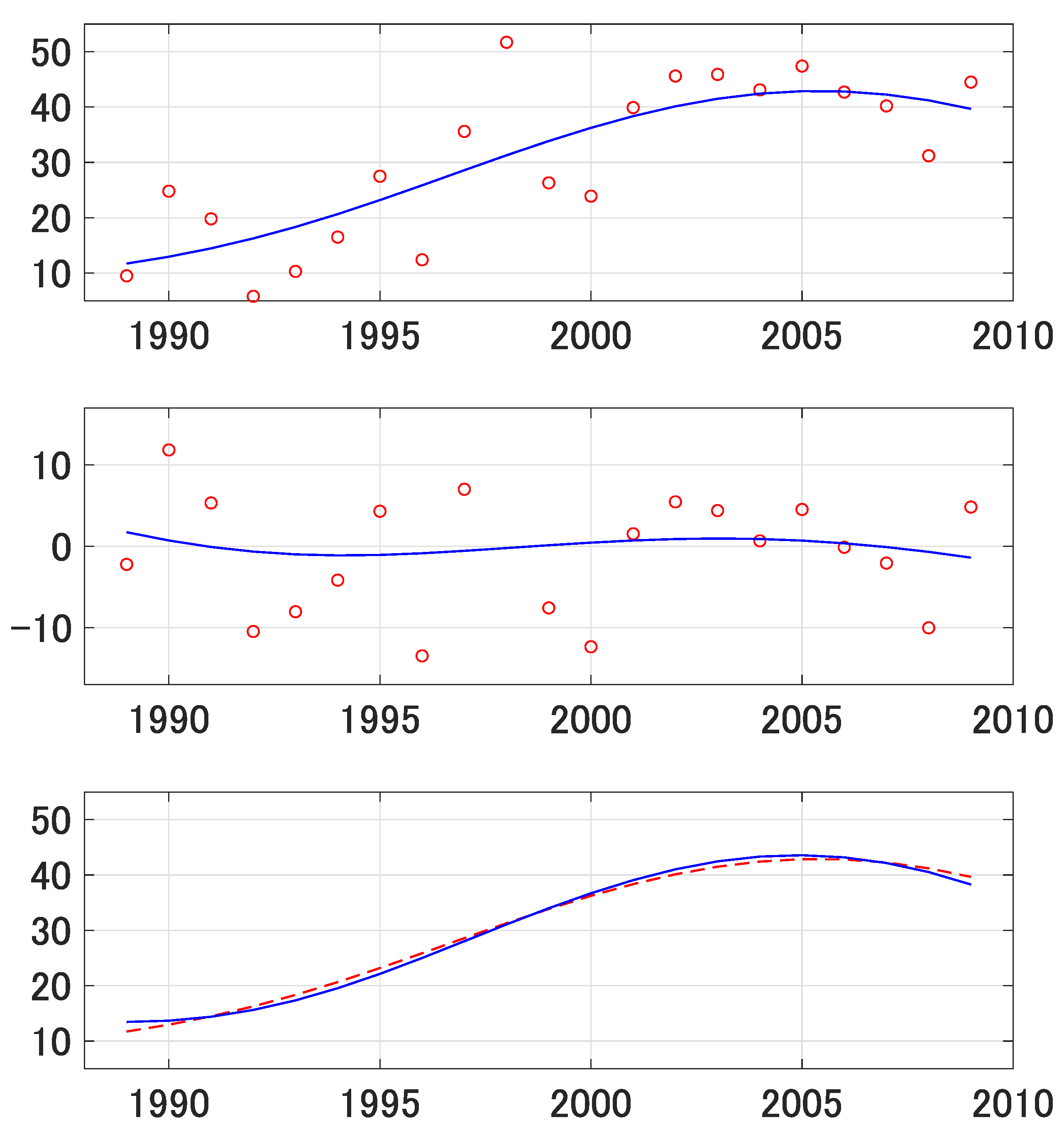
Figure 4 shows the results for the case where ${\lambda }_p={10}^6$ and $p=3$. The top panel shows $\mathit{y}$ (red circle) and ${\widehat{\mathit{x}}}_p^{\left(1\right)}(={\widehat{\mathit{x}}}_p)$ (blue solid line). Since the value of ${\lambda }_p$ is huge, from Proposition 1(v), it follows that

$$\begin{array}{c}\hfill {\widehat{\mathit{x}}}_p^{\left(1\right)}\approx {\widehat{\mathit{\tau }}}_p={\mathbf{\Pi }}_p{\left({\mathbf{\Pi }}_p^{\top }{\mathbf{\Pi }}_p\right)}^{-1}{\mathbf{\Pi }}_p^{\top }\mathit{y}.\end{array}$$

(61)

Alternatively, we can see this as the result of the following fact:

$$\begin{array}{cc}\hfill {\mathit{A}}_p^{\left(1\right)}& ={\mathit{A}}_p={({\mathit{I}}_n+{\lambda }_p{\mathbf{\Delta }}_p^{\top }{\mathbf{\Delta }}_p)}^{-1}={\mathit{I}}_n-{\mathbf{\Delta }}_p^{\top }{\left({\displaystyle \frac{1}{{\lambda }_p}}{\mathit{I}}_{n-p}+{\mathbf{\Delta }}_p{\mathbf{\Delta }}_p^{\top }\right)}^{-1}{\mathbf{\Delta }}_p\hfill \\ \hfill & \approx {\mathit{I}}_n-{\mathbf{\Delta }}_p^{\top }{\left({\mathbf{\Delta }}_p{\mathbf{\Delta }}_p^{\top }\right)}^{-1}{\mathbf{\Delta }}_p={\mathbf{\Pi }}_p{\left({\mathbf{\Pi }}_p^{\top }{\mathbf{\Pi }}_p\right)}^{-1}{\mathbf{\Pi }}_p^{\top },\hfill \end{array}$$

(62)

if ${\lambda }_p$ is huge. Here, the third equality follows from the Sherman–Morrison–Woodbury formula to ${({\mathit{I}}_n+{\lambda }_p{\mathbf{\Delta }}_p^{\top }{\mathbf{\Delta }}_p)}^{-1}$. The last equality follows from the fact that $[{\mathbf{\Pi }}_p,{\mathbf{\Delta }}_p^{\top }]$ is nonsingular and ${\left({\mathbf{\Delta }}_p^{\top }\right)}^{\top }{\mathbf{\Pi }}_p={\mathbf{\Delta }}_p{\mathbf{\Pi }}_p={\mathbf{0}}_{n-p,p}$. The middle panel shows $\mathit{y}-{\widehat{\mathit{x}}}_p^{\left(1\right)}$ (red circle) and ${\mathit{A}}_p^{\left(1\right)}(\mathit{y}-{\widehat{\mathit{x}}}_p^{\left(1\right)})$ (blue solid line). From the panel, it is observable that

$$\begin{array}{c}\hfill {\mathit{A}}_p^{\left(1\right)}(\mathit{y}-{\widehat{\mathit{x}}}_p^{\left(1\right)})\approx {\mathbf{0}}_{n,1},\end{array}$$

(63)

which shows that there is no gain from boosting if ${\lambda }_p$ is huge. The result is reasonable from

$$\begin{array}{c}\hfill {\mathbf{\Pi }}_p{\left({\mathbf{\Pi }}_p^{\top }{\mathbf{\Pi }}_p\right)}^{-1}{\mathbf{\Pi }}_p^{\top }\left\{{\mathit{I}}_n-{\mathbf{\Pi }}_p{\left({\mathbf{\Pi }}_p^{\top }{\mathbf{\Pi }}_p\right)}^{-1}{\mathbf{\Pi }}_p^{\top }\right\}={\mathbf{0}}_{n,n}.\end{array}$$

The bottom panel shows ${\widehat{\mathit{x}}}_p^{\left(1\right)}$ (red dashed line) and ${\widehat{\mathit{x}}}_p^{\left(2\right)}$ (blue solid line). In this case, since

$$\begin{array}{c}\hfill {\widehat{\mathit{x}}}_p^{\left(2\right)}={\widehat{\mathit{x}}}_p^{\left(1\right)}+{\mathit{A}}_p^{\left(1\right)}(\mathit{y}-{\widehat{\mathit{x}}}_p^{\left(1\right)})\approx {\widehat{\mathit{x}}}_p^{\left(1\right)},\end{array}$$

(64)

we cannot observe the red dashed line in the panel. Note that the first equality in (64) follows from (31).

Figure 5 shows the results for the case where ${\lambda }_p=1160$ and $p=3$, where ${\lambda }_p=1160$ is the value used in Nocon and Scott (2012) [6]. They selected the value by using generalized cross-validation. Again, the top panel shows $\mathit{y}$ (red circle) and ${\widehat{\mathit{x}}}_p^{\left(1\right)}$ (blue solid line). The middle panel shows $\mathit{y}-{\widehat{\mathit{x}}}_p^{\left(1\right)}$ (red circle) and ${\mathit{A}}_p^{\left(1\right)}(\mathit{y}-{\widehat{\mathit{x}}}_p^{\left(1\right)})$ (blue solid line). From the middle panel, it is observable that

$$\begin{array}{c}\hfill {\mathit{A}}_p^{\left(1\right)}(\mathit{y}-{\widehat{\mathit{x}}}_p^{\left(1\right)})\ne {\mathbf{0}}_{n,1}.\end{array}$$

(65)

Recall that ${\mathit{A}}_p^{\left(1\right)}(\mathit{y}-{\widehat{\mathit{x}}}_p^{\left(1\right)})$ is the gain from boosting. Given that ${\widehat{\mathit{x}}}_p^{\left(2\right)}={\widehat{\mathit{x}}}_p^{\left(1\right)}+{\mathit{A}}_p^{\left(1\right)}(\mathit{y}-{\widehat{\mathit{x}}}_p^{\left(1\right)})$, due to this gain from boosting, in the bottom panel, ${\widehat{\mathit{x}}}_p^{\left(2\right)}$ (blue solid line) is different from ${\widehat{\mathit{x}}}_p^{\left(1\right)}$ (red dashed line). In addition, we report the following two results:

$$\begin{array}{c}{\displaystyle \frac{1}{n}}{\mathit{\iota }}^{\top }\mathit{y}={\displaystyle \frac{1}{n}}{\mathit{\iota }}^{\top }{\widehat{\mathit{\tau }}}_p={\displaystyle \frac{1}{n}}{\mathit{\iota }}^{\top }{\widehat{\mathit{x}}}_p^{\left(1\right)}={\displaystyle \frac{1}{n}}{\mathit{\iota }}^{\top }{\widehat{\mathit{x}}}_p^{\left(2\right)}=30.695,\\ {\displaystyle \frac{1}{n}}{\mathit{\iota }}^{\top }\left\{{\mathit{A}}_p^{\left(1\right)}(\mathit{y}-{\widehat{\mathit{x}}}_p^{\left(1\right)})\right\}=0.\end{array}$$

These are consistent with Proposition 1(i).

We also tried the case where ${\lambda }_p={10}^{-6}$ and $p=3$. In the case, we obtained the following:

$$\begin{array}{c}{\widehat{\mathit{x}}}_p^{\left(m\right)}\approx \mathit{y},m=1,2,\end{array}$$

(66)

$$\begin{array}{c}{\mathit{A}}_p^{\left(1\right)}(\mathit{y}-{\widehat{\mathit{x}}}_p^{\left(1\right)})\approx {\mathbf{0}}_{n,1},\end{array}$$

(67)

which are consistent with Proposition 1(vi).

6. Concluding Remarks

In this paper, we developed the boosted version of the WH graduation and established its properties. The theoretical results we obtained are summarized in Proposition 1 and Lemmas 1 and 2 and empirically illustrated in Section 5. Also see

Table 1. List of the relationships between the main matrices.

	WH(p) Graduation	bWH(p) Graduation
Smoother matrix	${\mathit{A}}_p$	${\mathit{A}}_p^{\left(m\right)}$
Spectral decomposition of smoother matrix	${\mathit{U}}_p{\mathit{B}}_p{\mathit{U}}_p^{\top }$	${\mathit{U}}_p{\mathit{B}}_p^{\left(m\right)}{\mathit{U}}_p^{\top }$
Penalty matrix	${\mathit{C}}_p$	${\mathit{C}}_p^{\left(m\right)}$
Spectral decomposition of penalty matrix	${\mathit{U}}_p{\mathit{D}}_p{\mathit{U}}_p^{\top }$	${\mathit{U}}_p{\mathit{D}}_p^{\left(m\right)}{\mathit{U}}_p^{\top }$

, which lists the relationships between the main matrices such as ${\mathit{A}}_p^{\left(m\right)}$ and ${\mathit{B}}_p^{\left(m\right)}$.

Finally, we give a remark. To use the bWH(p) graduation in (27), the values of the three parameters, p, ${\lambda }_p$, and m, must be specified. Among them, the specification of ${\lambda }_p$ is particularly important. This is because, as empirically shown in Section 5, ${\widehat{\mathit{x}}}_p^{\left(m\right)}$ is strongly dependent on the value of ${\lambda }_p$. One idea is to determine the value of ${\lambda }_p$ using the (approximate) gain function corresponding to the smoother matrix, ${\mathit{A}}_p(={\mathit{A}}_p^{\left(1\right)})$. However, it seems better to determine it by also considering the value of m. This could be achieved by extending the approach adopted by Hall and Thomson (2024) [13]. We are investigating this issue and will report our findings in the future.

References

1. Bohlmann, G. Ein Ausgleichungsproblem. Nachrichten von der Gesellschaft der Wissenschaften zu Gottingen Mathematisch-Physikalische Klasse 1899, 1899, 260–271. [Google Scholar]
2. Hodrick, R.J.; Prescott, E.C. Postwar U.S. business cycles: An empirical investigation. J. Money Credit. Bank. 1997, 29, 1–16. [Google Scholar] [CrossRef]
3. Whittaker, E.T. On a new method of graduation. Proc. Edinb. Math. Soc. 1923, 41, 63–75. [Google Scholar] [CrossRef]
4. Weinert, H.L. Efficient computation for Whittaker–Henderson smoothing. Comput. Stat. Data Anal. 2007, 52, 959–974. [Google Scholar] [CrossRef]
5. Phillips, P.C.B. Two New Zealand pioneer econometricians. N. Z. Econ. Pap. 2010, 44, 1–26. [Google Scholar]
6. Nocon, A.S.; Scott, W.F. An extension of the Whittaker–Henderson method of graduation. Scand. Actuar. J. 2012, 1, 70–79. [Google Scholar] [CrossRef]
7. Biessy, G. Revisiting Whittaker–Henderson smoothing. arXiv 2023, arXiv:2306.06932. [Google Scholar]
8. Phillips, P.C.B.; Shi, Z. Boosting: Why you can use the HP filter. Int. Econ. Rev. 2021, 62, 521–570. [Google Scholar] [CrossRef]
9. Yamada, H. Linear trend, HP trend, and bHP trend. SSRN 2024. [Google Scholar] [CrossRef]
10. Knight, K. The Boosted Hodrick–Prescott Filter, Penalized Least Squares, and Bernstein Polynomials. Unpublished Manuscript. 2021. Available online: https://utstat.utoronto.ca/keith/papers/hp-pls.pdf (accessed on 26 October 2024).
11. Tomal, M. Testing for overall and cluster convergence of housing rents using robust methodology: Evidence from Polish provincial capitals. Empir. Econ. 2022, 62, 2023–2055. [Google Scholar] [CrossRef] [PubMed]
12. Trojanek, R.; Gluszak, M.; Kufel, P.; Tanas, J.; Trojanek, M. Pre and post-financial crisis convergence of metropolitan housing markets in Poland. J. Hous. Built Environ. 2023, 38, 515–540. [Google Scholar] [CrossRef]
13. Hall, V.B.; Thomson, P. Selecting a boosted HP filter for growth cycle analysis based on maximising sharpness. J. Bus. Cycle Res. 2024. [Google Scholar] [CrossRef]
14. Mei, Z.; Phillips, P.C.B.; Shi, Z. The boosted Hodrick–Prescott filter is more general than you might think. J. Appl. Econom. 2024. [Google Scholar] [CrossRef]
15. Biswas, E.; Sabzikar, F.; Phillips, P.C.B. Boosting the HP filter for trending time series with long-range dependence. Econom. Rev. 2024. [Google Scholar] [CrossRef]
16. Yamada, H. Boosted HP filter: Several properties derived from its spectral representation. In Computational Science and Its Applications—ICCSA 2024; Gervasi, O., Murgante, B., Garau, C., Taniar, D., C. Rocha, A.M.A., Faginas Lago, M.N., Eds.; Springer: Cham, Switzerland, 2024. [Google Scholar] [CrossRef]
17. Bao, R.; Yamada, H. Boosted Whittaker–Henderson Graduation of Order 1: A Graph Spectral Filter Using Discrete Cosine Transform. Contemp. Math. 2024. Forthcoming. Available online: https://www.researchgate.net/publication/384363420_Boosted_Whittaker-Henderson_Graduation_of_Order_1_A_Graph_Spectral_Filter_Using_Discrete_Cosine_Transform (accessed on 26 October 2024).
18. Anderson, T.W. The Statistical Analysis of Time Series; John Wiley and Sons: New York, NY, USA, 1971. [Google Scholar]
19. Strang, G. The discrete cosine transform. SIAM Rev. 1999, 41, 135–147. [Google Scholar] [CrossRef]
20. Nakatsukasa, Y.; Saito, N.; Woei, E. Mysteries around the graph Laplacian eigenvalue 4. Linear Algebra Its Appl. 2013, 438, 3231–3246. [Google Scholar] [CrossRef]
21. Kim, S.; Koh, K.; Boyd, S.; Gorinevsky, D. 1 trend filtering. SIAM Rev. 2009, 51, 339–360. [Google Scholar] [CrossRef]
22. Yamada, H. A smoothing method that looks like the Hodrick–Prescott filter. Econom. Theory 2020, 36, 961–981. [Google Scholar] [CrossRef]
23. Yamada, H. Why does the trend extracted by the Hodrick–Prescott filtering seem to be more plausible than the linear trend? Appl. Econ. Lett. 2018, 25, 102–105. [Google Scholar] [CrossRef]
Figure 1. Eigenvalues d p , 1 , , d p , n for p = 3 and n = 50 .
Mathematics 12 03377 g001
Figure 2. Eigenvectors u p , 4 , u p , 8 , u p , 12 , u p , 16 for p = 3 and n = 50 .
Mathematics 12 03377 g002
Figure 3. Eigenvalues b p , 1 ( m ) , , b p , n ( m ) for p = 3 , n = 50 , m = 2 , and λ p = 1000 .
Mathematics 12 03377 g003
Figure 4. Empirical illustration. λ p = 10 6 and p = 3 . The top panel shows y (red circle) and x ^ p ( 1 ) ( = x ^ p ) (blue solid line). The middle panel shows y x ^ p ( 1 ) (red circle) and A p ( 1 ) ( y x ^ p ( 1 ) ) (blue solid line). The bottom panel shows x ^ p ( 1 ) (red dashed line) and x ^ p ( 2 ) (blue solid line).
Mathematics 12 03377 g004
Figure 5. Empirical illustration. λ p = 1160 and p = 3 . The top panel shows y (red circle) and x ^ p ( 1 ) ( = x ^ p ) (blue solid line). The middle panel shows y x ^ p ( 1 ) (red circle) and A p ( 1 ) ( y x ^ p ( 1 ) ) (blue solid line). The bottom panel shows x ^ p ( 1 ) (red dashed line) and x ^ p ( 2 ) (blue solid line).
Mathematics 12 03377 g005