Abstract
The portfolio selection problem has been a central focus in financial research. A complete portfolio selection process includes two stages: stock pre-selection and portfolio optimization. However, most existing studies focus on portfolio optimization, often overlooking stock pre-selection. To address this problem, this paper presents a novel two-stage approach that integrates deep learning with portfolio optimization. In the first stage, we develop a stock trend prediction model for stock pre-selection called the AGC-CNN model, which leverages a convolutional neural network (CNN), self-attention mechanism, Graph Convolutional Network (GCN), and k-reciprocal nearest neighbors (k-reciprocal NN). Specifically, we utilize a CNN to capture individual stock information and a GCN to capture relationships among stocks. Moreover, we incorporate the self-attention mechanism into the GCN to extract deeper data features and employ k-reciprocal NN to enhance the accuracy and robustness of the graph structure in the GCN. In the second stage, we employ the Global Minimum Variance (GMV) model for portfolio optimization, culminating in the AGC-CNN+GMV two-stage approach. We empirically validate the proposed two-stage approach using real-world data through numerical studies, achieving a roughly 35% increase in Cumulative Returns compared to portfolio optimization models without stock pre-selection, demonstrating its robust performance in the Average Return, Sharp Ratio, Turnover-adjusted Sharp Ratio, and Sortino Ratio.
MSC:
68T07; 68U10
1. Introduction
For investors aiming to maximize profits while minimizing risk, portfolio optimization has long been recognized as an effective strategy and is one of the major research topics in the financial field [1,2]. This paper focuses on selecting appropriate investment assets and allocating investors’ wealth across various assets, thus creating a productive investment strategy for investors. In precise terms, a comprehensive investment process consists of two stages: stock pre-selection and portfolio optimization [3]. The first stage is to analyze assets by integrating individual stock information and relationships among stocks to determine which ones have investment value, formulating a stock pre-selection model. The second stage is an optimization problem that aims to offer investors a reliable allocation of portfolio weights to maximize returns while minimizing risks.
In actual portfolio selection, we need to first conduct stock pre-selection because the quantity of stock holdings within the optimal portfolio is limited and the failure to select suitable assets may yield suboptimal portfolios that fail to align with investment objectives [4]. However, the existing studies predominantly concentrate on portfolio optimization, assuming that stock pre-selection is ignored or has already been conducted [5,6]. Yang et al. [7] pointed out that the efficacy of portfolio selection heavily relies on the future performance of stocks, and accurate predictions may lead to higher returns and lower risks. Therefore, it is crucial to conduct stock pre-selection by predicting the future performance of stocks. Because of the nature of stock data, such as having rapid changes, having non-linearity, being non-parametric, and their chaotic nature, predicting the future performance of stocks has always been a challenging task. Certain studies seek to forecast future stock prices or returns using regression techniques [8,9], whereas other studies emphasize predicting the future direction of stock price trends through classification approaches [10]. However, for stock pre-selection, the greater focus is on the stock trend prediction. How to conduct stock pre-selection through stock trend prediction is a key issue to be addressed in this paper.
In recent years, machine learning techniques have become a prevailing trend in handling stock trend prediction [11]. Previous studies [12,13] have demonstrated the efficacy of machine learning in addressing non-stationary and non-linear data compared to traditional statistical strategies. Deep learning is a frequently employed machine learning technique for predicting stock trends, adept at uncovering non-linear and non-additive relationships within data [14], such as the recurrent neural network (RNN) [15], convolutional neural network (CNN) [16,17], and long short-term memory network (LSTM) [18,19]. Among the aforementioned deep learning models, the CNN stands out for its remarkable performance, leveraging convolution layers to effectively capture essential features [20]. Many researchers have adopted the approach of transforming stock data into visual representations and then utilizing a CNN to obtain multi-scale localized spatial characteristics for predicting stock trends. Wu et al. [21] introduced a graph-based CNN-LSTM architecture that employed a mix of diverse images, including options, futures, and historical data. Jiang et al. [22] extracted trading signals from OHLC chart images and analyzed them using Dual-CNN, demonstrating that forecasts utilizing image data typically surpass traditional signals of price trends in the asset pricing literature.
A CNN is constrained to processing data organized on regular grids and struggles to effectively capture intricate topological structures [23,24]. Specifically, a CNN can only capture individual stock data and fails to capture the relationships among stocks. To solve this problem, Kipf and Welling [25] introduced a groundbreaking deep learning technique known as Graph Convolutional Network (GCN). In recent years, GCN has found widespread application in the financial sector and are often integrated with other deep learning models. Wang et al. [26] proposed an index trend prediction model based on a multi-graph convolutional neural network, named MG-Conv. Li et al. [27] developed an LSTM-RGCN model that utilized the correlation matrix to capture both positive and negative relationships between stocks.
The application of GCN requires the provision of both a feature matrix and adjacency matrix. Given the heightened complexity, disorderliness, and non-linearity in stock market data, directly extracting features from raw stock data to generate feature matrices presents inherent limitations. To address this challenge, the self-attention mechanism proposed by Vaswani et al. [28] offers a solution by capturing deep-seated features within the stock data, and it has gradually extended to the financial sector [29,30]. Li et al. [31] employed the attention mechanism to tackle the challenges of temporal dependency in financial data, proposing an innovative Transformer encoder attention (TEA) model. Similarly, Wang et al. [32] presented a novel policy gradient trading algorithm named DeepTrader, featuring a Market Scoring Unit and an Asset Scoring Unit. The Asset Scoring Unit utilizes the dilated CNN and attention mechanisms to extract temporal and spatial features across assets, while also integrating a GCN to model interrelationships and causal relationships among them. Additionally, GCN utilizes a complete adjacency matrix to depict relationships among different stocks in the stock market. However, this approach may face challenges such as a high computational complexity and large storage requirements, especially when handling extensive stock data. To mitigate this issue, the k-reciprocal NN algorithm is proposed to streamline the adjacency matrix of a GCN. The k-reciprocal NN is a technique commonly employed to enhance nearest neighbor searches, particularly in the domains of computer vision and image retrieval [33,34]. By leveraging k-reciprocal NN, it becomes feasible to significantly simplify the representation of the adjacency matrix while retaining crucial connections among stocks. Specifically, the k-reciprocal NN algorithm can filter out the k most relevant neighbors for each stock and subsequently establish a simplified adjacency matrix based on these neighbors, thereby achieving a more efficient encoding of relationships among stocks.
After completing stock pre-selection with the stock trend prediction model, the second stage of a complete investment process, portfolio optimization, is also a critical issue. Regarding this issue, the GMV model is generally considered as an effective strategy [35,36]. The GMV model simplifies portfolio optimization by solely relying on the covariance matrix, which can be broken down into a variance–correlation form, representing the product of a diagonal variance matrix and a correlation matrix. Variance and correlation, fundamental metrics in financial analysis, are employed to measure the risk and correlation of asset returns, respectively. The GMV model solves the optimization problem in the second stage of a complete investment process, providing investors with an effective portfolio weight allocation based on the determination of assets with investment value in the first stage.
In this paper, we covered two key stages of an investment process, analyzing assets to determine which ones have investment value and providing investors with an effective portfolio weight allocation. In the first stage, we proposed a stock trend prediction model for stock pre-selection: the AGC-CNN model, which simultaneously employs a CNN to capture individual stock information and uses a GCN to model relationships among stocks. Furthermore, we leverage self-attention to optimize the feature matrix of the GCN, identifying deep-seated features within the stock data. Meanwhile, we utilize k-reciprocal NN to significantly simplify the representation of an adjacency matrix of a GCN while retaining crucial connections among stocks. This allows for a more efficient encoding of stock market information, improving the accuracy and robustness of the GCN graph structure. In the second stage, we use the GMV model to provide investors with an effective portfolio weight allocation. Subsequently, by incorporating the AGC-CNN model and GMV model, we finalize this model as the AGC-CNN+GMV two-stage approach.
The primary contributions can be outlined as follows:
- Leveraging the self-attention mechanism and k-reciprocal NN to optimize the feature matrix and adjacency matrix of a GCN, respectively.
- The development of OHLC (open, high, low, close) charts from the ground up, alongside the construction of a dual-layer CNN model utilizing the LeakyReLU activation function.
- The simultaneous integration of a CNN and GCN to capture both individual stock information and relationships among stocks, culminating in the creation of the AGC-CNN model for stock pre-selection.
- The integration of the AGC-CNN model with the GMV model, establishing a two-stage approach where high-quality stocks are initially identified, followed by portfolio selection optimization.
The rest of this paper is structured as follows: Section 2 offers related studies, exploring key concepts pertinent to the proposed model. Section 3 details the specifics of the proposed model. In Section 4, we present the experimental setup and process. Section 5 examines the experimental results. Section 6 provides a summary of this paper, outlining the key points discussed and suggesting directions for future improvements.
2. Preliminary Work
2.1. The Global Minimum Variance
Suppose we have N stocks, and denotes the vector of asset returns at time t. The traditional GMV model, given an weight vector , aims to find the minimum risk of the portfolio:
where is an unit vector and is an covariance matrix. The optimal weight for Equation (1) can be obtained as follows:
However, the true covariance matrix is unknown, which can be replaced by the sample covariance matrix , meaning that
In the above Equation (2), and .
2.2. The Convolutional Neural Network
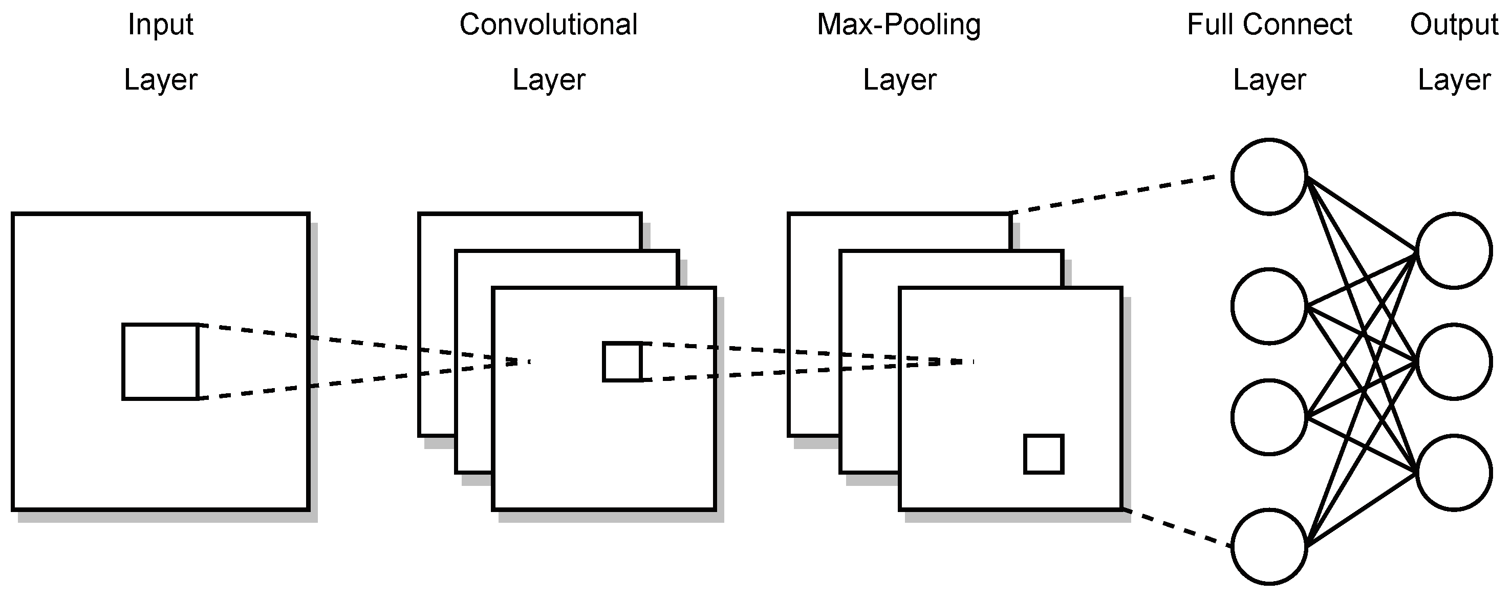
The core principle of the CNN is its modularity, with core building blocks comprising three operations: convolution, pooling, and activation layer. Figure 1 shows a schematic diagram of the CNN. The convolution layer, which comprises a set of filters represented by a low-dimensional kernel weight matrix, is the core operation in a CNN. These filters move across the input data, executing convolution operations to extract features. During the training process, the weights of filters are initialized at random and progressively refined using the training set through the learning process. The convolution operation can be represented by the following equation:
where and represent the feature outputs of the i and layers, respectively. represents the weight vector, ∗ indicates the convolution operation, and signifies the bias term of the i-th layer.
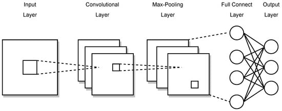
Figure 1.
Schematic diagram of CNN structure.
2.3. The Graph Convolutional Network
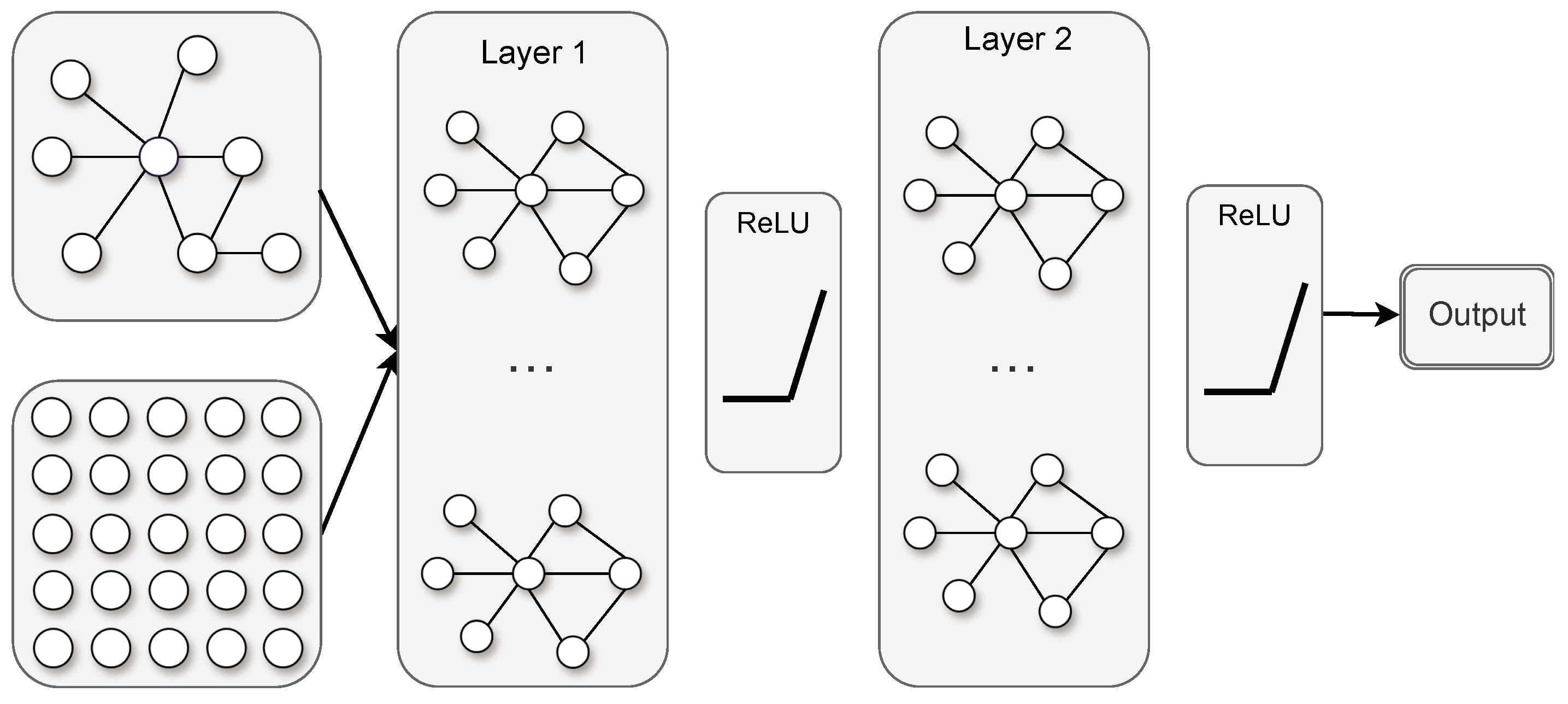
Due to its ability to handle irregular data structures, GCNs serve an essential role in stock market prediction. Figure 2 presents a schematic diagram of a GCN. The pivotal component of a GCN is the graph convolutional layer, which conducts convolution operations on the graph structure. The design of this layer is crucial as it enables the GCN to effectively capture the intricate relationships among nodes in graph data. As mentioned earlier, suppose we have N stocks, where each stock records D features. Each stock is represented as a node, and each node comprises D features. The node features collectively form an feature matrix X, while the relationships among nodes are depicted by an adjacency matrix A. The feature matrix X and the adjacency matrix A function as inputs to our model. The propagation formula for the graph convolutional layer is as follows:
where and represent the non-linear activation function and the trainable weights, respectively. is the degree matrix of (). Additionally, denotes the features at the lth layer, and for the input layer, is equal to X.
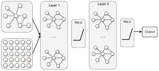
Figure 2.
Schematic diagram of GCN structure.
2.4. Self-Attention Mechanism
Figure 3 displays a schematic representation of self-attention. We consider the graph structure formed by stock data, where each stock is regarded as a node. Each node has D features, and the features of all stocks form the feature matrix . Each node i possesses a feature vector , and we utilize learned weights , , and to map them to query , key , and value . Attention weights are computed by measuring the similarity among queries and keys. Then, scaling is applied to obtain the following: , where is the dimensionality of the query or key. This scaling operation helps to avoid problems with disappearing gradients or exploding gradients. The softmax function is then applied to generate normalized attention weights: . Finally, the values of the nodes are summed using the attention weights, resulting in the ultimate feature vector representation :

Figure 3.
Schematic diagram of self-attention.
Translating this into vector form:
where , , and are vector forms of q, k, and v, respectively.
2.5. k-Reciprocal Nearest Neighbors
The fundamental concept of k-reciprocal NN is that when searching for the k nearest neighbors of a point, it not only factors in the distances of these k points to the target point but also ensures that each of these k points regard the target point as one of its nearest neighbors. Following Qin et al. [34], the k nearest neighbors of stock q, representing the top k samples from the ranking list, are denoted by .
Then, the k-reciprocal NN can be specified as
The advantage of k-reciprocal NN lies in its emphasis on the mutual verification of relationships. By mandating that nearest neighbors are mutual, this method effectively eliminates imprecise nearest neighbor results stemming from noise or specific data distributions, offering a more reliable performance when handling stock relationship graphs.
3. Method
3.1. The Stock Pre-Selection Model
This section presents the AGC-CNN model designed to predict stock trends and select high-quality stocks. The proposed AGC-CNN model consists of four primary steps: image creation, capturing individual stock information using a CNN, capturing information among stocks using a GCN, and constructing the AGC-CNN model by combining a CNN and GCN.
3.1.1. Image Creation
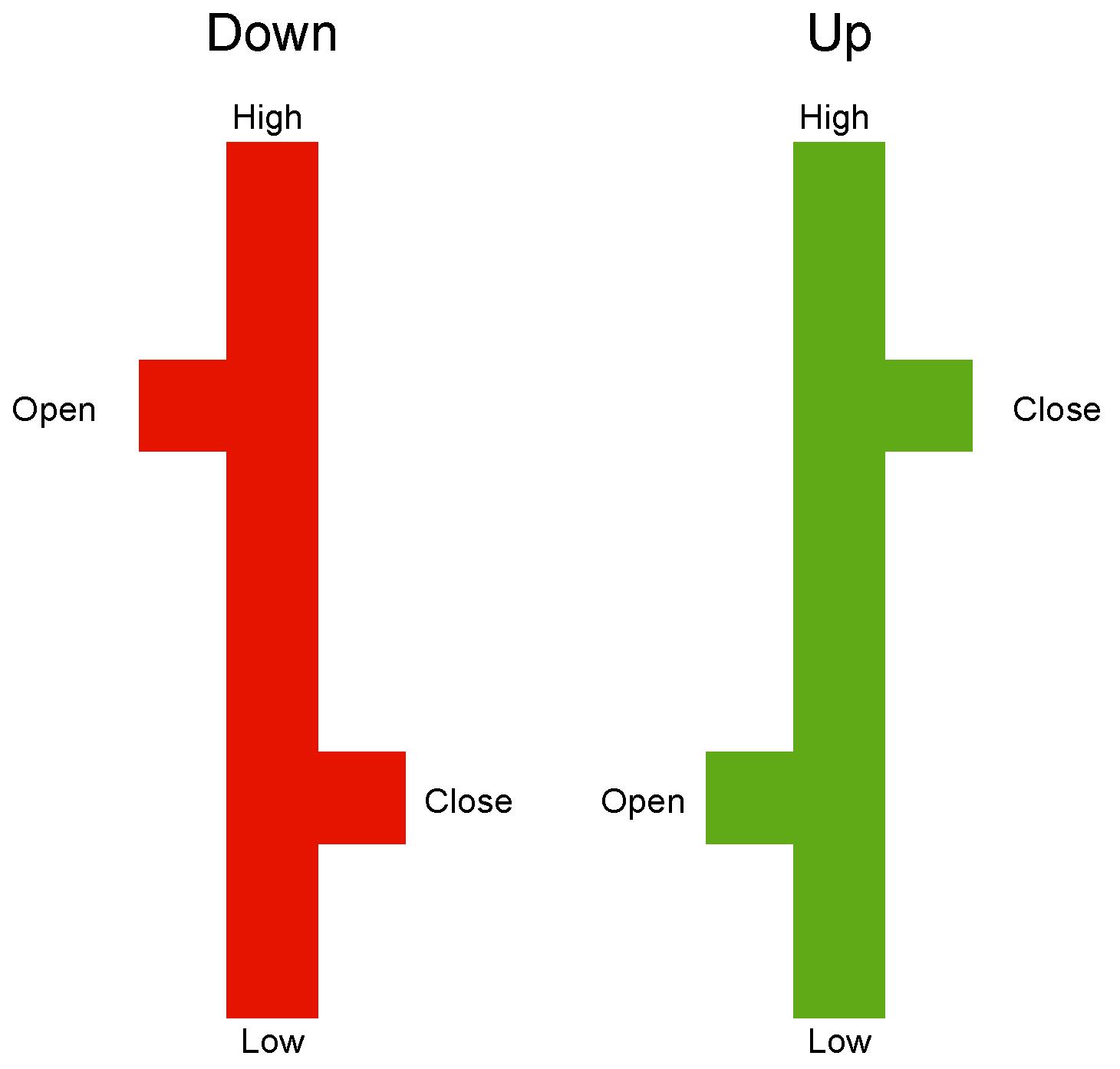
This section discusses how historical market data are represented as input images for the CNN. We create our own charts from the ground up, as detailed in Jiang et al. [22], primarily employing OHLC bar charts. As depicted in Figure 4, the high and low prices on the chart are represented by the top and bottom of the central vertical line, whereas the open and close prices are shown by small horizontal lines extending to the left and right of the vertical line.

Figure 4.
The OHLC chart.
Our images primarily consist of consecutive daily OHLC bars spanning five days (approximately a week). For each image, we applied normalization to the open, close, high, and low prices, ensuring that all values are scaled within the range of 0 to 1. Additionally, to ensure consistency, we keep a uniform height for all images and adjust the vertical axis to ensure that images representing the same number of days have identical pixel scales.
To enrich the OHLC charts, we introduce two supplementary information items: the moving average line and daily trading volume. The moving average line is a valuable tool in traditional technical analysis, offering a long-term reference point for current prices. We set the window width of the moving average equivalent to the quantity of days represented in the images. The daily moving average line is represented using the pixels in the middle column of each day, forming a connected line through these points. The second additional information is the daily trading volume, depicted as volume bars. The volume is shown at the bottom fifth of the image, while the top four-fifths encompass the OHLC chart and the moving average line. Figure 5 shows examples from the final image datasets.

Figure 5.
Stock data images for 5 days. Note: black–white images are used in the experiments, and the red parts in the examples are only for the readers’ convenience in identifying the moving average lines.
Additionally, to simplify data storage requirements, we chose to use black and white instead of color. Black serves as the background color, while white is used for visible objects on the chart. This means that most of the space on the chart is black, as the RGB value for black pixels is (0, 0, 0), resulting in a sparse image. At the same time, the direction of price changes is indicated by the markers for opening and closing prices. This allows us to focus on the 2D pixel matrix without having to track the third dimension of RGB pixel intensity.
3.1.2. Capturing Individual Stock Information Using CNN
As illustrated in Figure 6, our model is constructed with two CNN modules, with an input size of . The first building block contains 64 filters, and the quantity of filters in each successive convolutional layer adheres to a pattern of doubling.

Figure 6.
The CNN structure diagram.
Given the sparsity of the image in the vertical dimension, we opted for convolutional filters and max-pooling filters. This choice helps effectively capture vertical features in the image and reduces data dimensions to enhance computational efficiency during the pooling stage. To introduce non-linearity, we chose LeakyReLU as the activation function. LeakyReLU, compared to traditional ReLU, has a small slope in the negative region, aiding in mitigating neuron saturation issues and promoting a more robust gradient flow for model learning. According to Equation (3), we can obtain the individual stock features using the following formula:
Remark 1.
The LeakyReLU activation function was proposed by Maas et al. [37]. As an enhancement of the conventional ReLU function, which nullifies negative signals while preserving positive ones, Leaky ReLU addresses two significant shortcomings of ReLU. Firstly, ReLU can cause unidirectional gradients, making optimization challenging during training when the input is exclusively positive. Secondly, ReLU may deactivate neurons indefinitely if their gradients consistently fall within the zero-valued domain of the function. By integrating a small, non-zero gradient through a coefficient for inactive neurons, Leaky ReLU effectively mitigates these limitations:
In this section, we utilize a CNN to capture individual stock information. However, as a CNN cannot handle complex topological structures, we introduce a GCN to capture relationships among stocks.
3.1.3. Capturing Relationships Among Stocks Using GCN
In the stock market network, each stock i is depicted as a node, with the correlations between stocks represented as edges. To achieve a more comprehensive understanding of market dynamics, we introduced innovative enhancements to a GCN. This is specifically divided into three main steps: improvement of the adjacency matrix, enhancement of the feature matrix, and construction of a GCN.
Step 1: Improvement of the adjacency matrix. This step involves establishing edges among nodes to facilitate a deeper comprehension of relationships among stocks. The edges between nodes are established based on the correlation of change rates from four datasets: open, close, high, and low price.
Taking the closing price as an example, we denote as the close price of stock i on time t, where . Next, we compute the return rate for each node in the network: . Additionally, we employ the Pearson correlation coefficient to illustrate the relationships among nodes, thereby defining the edges among nodes:
where and , which denote the change rate of the close price of two stocks. and indicate the average values of X and Y, respectively. By adhering to this procedure, the correlation coefficients matrix of the close price among all nodes can be represented as follows:
Next, we apply k-reciprocal NN to the matrix to improve the accuracy and robustness of the graph structure. We define as the k nearest neighbors, and we denote as the k-reciprocal NN of stock q:
where ∧ represents the intersection. By performing the above operation and processing using k-reciprocal NN, we obtain a new correlation coefficients matrix . The same process is applied to the open price, high price, and low price to obtain , , and . The final adjacency matrix is defined as
Step 2. Enhancement of feature matrix. Due to the heightened complexity, disorderliness, and non-linearity of stock market data, directly extracting features from raw stock information to create a feature matrix for application in GCNs presents inherent constraints. To enhance the feature matrix, we employ a self-attention mechanism with the following specific steps:
- Firstly, each stock i is represented as a node and has a feature vector . We use trained weight matrices , , and to map them to query , key , and value .
- Secondly, computing the attention weights by measuring the similarity among queries and keys and scaling is applied to obtain .
- Thirdly, the values of the nodes are weighted and summed using the attention weights, resulting in the ultimate representation : .
- Finally, all nodes are processed to obtain the feature matrix .
Step 3. Construction of GCN model. As shown in Figure 7, we construct a double-layer convolutional operation. The equation for the convolutional operation is expressed as follows:

Figure 7.
The GCN structure diagram.
3.1.4. Constructing the AGC-CNN Model by Combining a CNN and GCN
In this section, we present the AGC-CNN model, leveraging a combination of a CNN and GCN.
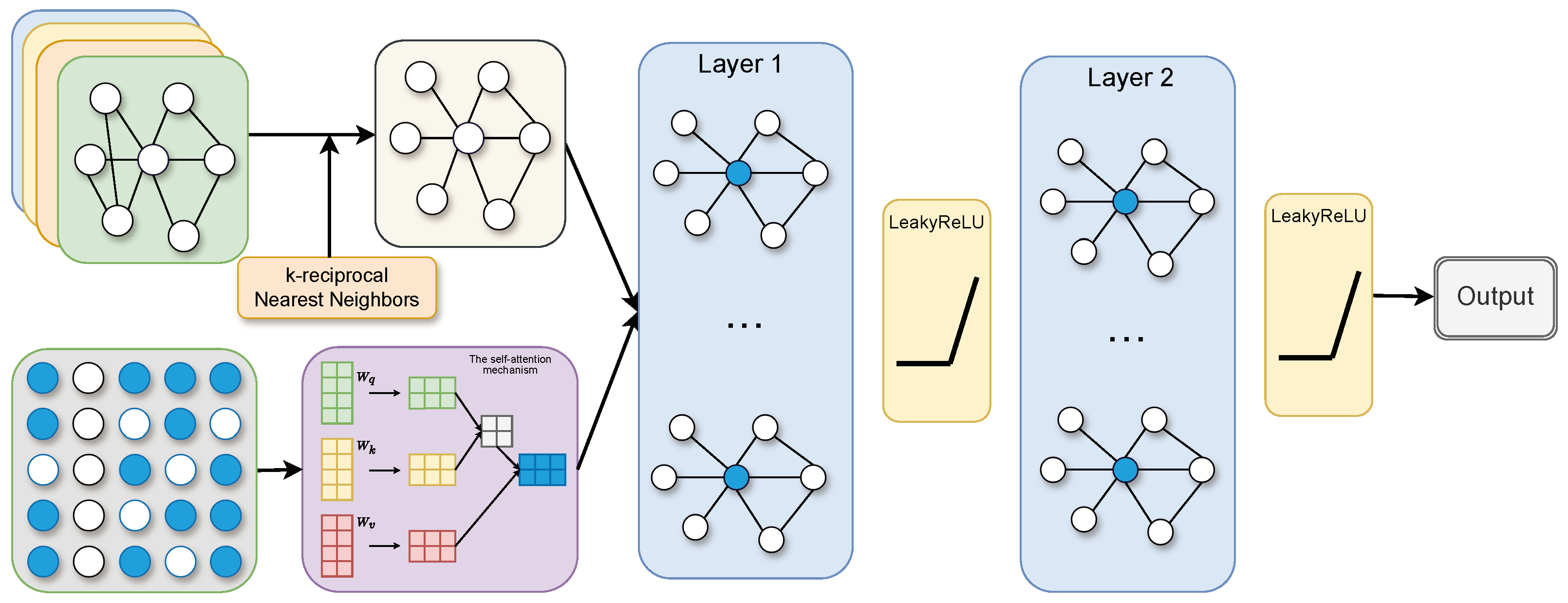
First, we use the stock price data (open, high, low, and close), along with two additional indicators, trading volume and moving averages, to construct the input for a CNN: OHLC charts. Through CNN processing (Section 3.1.2), we capture individual stock information, obtaining the result: .
Next, based on the same stock price data (open, high, low, and close), we construct the feature matrix X and the adjacency matrix A. We apply the self-attention mechanism to extract deep features from the feature matrix X and use k-reciprocal NN to process the adjacency matrix A, resulting in and , respectively, as inputs to the GCN. Through GCN processing (Section 3.1.3), we capture the relationships among stocks, obtaining the result: .
Finally, the individual stock features from the CNN and the features among stocks from a GCN are merged into joint features . The outputs can be represented as
where the represents the probabilities of up. W is the learnable weight matrix and b is the bias parameter.
Additionally, the predicted stock trend can be obtained using the following formula:
where 0 represents a predicted downward trend for the stock while 1 represents an upward trend.
3.2. Portfolio Optimization by Using the GMV Model
In the prior section, we predicted the stocks trend and proposed a stock pre-selection model to choose high-quality stocks from the stock pool. Suppose we selected p high-quality stocks. According to Equation (2), we can obtain the weight vector:
where refers to the covariance matrix derived from p high-quality stocks.
In this paper, we first conduct meticulous stock pre-selection through the AGC-CNN model, then optimize using the GMV model. This strategy establishes our methodology as a comprehensive two-stage approach, as shown in Figure 8. This two-stage approach, which not only rigorously addresses stock pre-selection but also ensures an optimized configuration aligned with our risk-return objectives, creates a more robust and efficient investment strategy.

Figure 8.
The AGC-CNN two-stage approach.
4. Experimental Process
This experiment encompasses two distinct parts: the first, dedicated to stock trend prediction, is executed using Python, while the second part, which centers on portfolio optimization, is conducted in R.
4.1. The Experiment of Stock Trend Prediction
4.1.1. Data Preparation
In the empirical analysis, we utilize daily stock data from CRSP for firms listed on NYSE, AMEX, and NASDAQ, covering the period from 1 January 2012 to 31 December 2023. We sort the stocks based on the missing value situation from 1 January 2012 to 1 December 2023, prioritizing those with fewer missing values to ensure data completeness and reliability. Since the GCN needs to capture the correlations between stocks, the stocks in the same batch must calculate the adjacency matrix. This requires that the stocks in the same batch cannot be repeated or omitted, ensuring that the characteristics of each stock can be fully utilized. Therefore, the number of selected stocks must match the batch size to meet the model input requirements. After tuning the model, we determine the batch size to be 128, which means that the 128 stocks with the fewest missing values are used in this experiment.
Finally, we conduct tests on four sets of data covering the periods 2012–2014, 2015–2017, 2018–2020, and 2021–2023, respectively. For each period, we randomly designate 70% of the samples as the training set, while the remaining 30% are assigned to the testing set.
4.1.2. Baseline Models
To assess the effectiveness of the stock trend prediction model proposed in this paper, we select several baseline models for comparison:
- FFNN: a basic model that learns patterns in stock data to predict stock trends.
- RNN [15]: capable of handling sequential stock data well, capturing time-based patterns to forecast future trends based on past performance.
- LSTM [18]: an advanced version of RNN, designed to remember long-term patterns in stock prices, making it suitable for predicting complex and long-term trends.
- GRU [38]: a simpler and efficient alternative to LSTM, which is capable of real-time trend prediction, useful for quick market response.
- CNN [16]: while commonly used for images, a CNN can process time series stock data to identify short-term trends and price movements.
- Dual-CNN [22]: a dual-layer CNN model, whose input is the same as that of a regular CNN.
- CNN + LSTM [21]: utilizes a CNN to obtain features across various time scales and uses LSTM to capture temporal dependencies in the features.
In addition, we conducted ablation studies:
- AGC-CNN without k-reciprocal NN: the proposed stock trend prediction (AGC-CNN) model does not apply k-reciprocal NN to the adjacency matrix.
- AGC-CNN without self-attention: the proposed stock trend prediction AGC-CNN model does not apply the self-attention mechanism to the feature matrix to extract deep features.
4.1.3. Evaluation Metrics
We consider the predictive analysis as a binary classification task, assigning a label of to images with positive returns, while those with non-positive returns are labeled as . The loss function we used is the cross-entropy loss function, specified as
where denotes the actual label of the i-th sample and indicates the predicted probability of up, calculated using Equation (7).
To evaluate the performance of different models in stock trends prediction, classification accuracy is chosen as the evaluation metric, which is specified as
In binary classification, a true positive (TP) occurs when a prediction with a probability above 50% aligns with an actual positive return, while a true negative (TN) is identified when a prediction with a probability below 50% corresponds with an actual negative return. False positives (FPs) and false negatives (FNs) represent the opposite scenarios, respectively.
4.2. The Experiment of Portfolio Optimization
4.2.1. Data Preparation
In the experiment for portfolio optimization, we utilize the same dataset as the one used in the stock trend prediction experiment. Throughout this process, we focus on extracting the close price of each stock and calculating its logarithmic return rate. Considering the continuous nature of time series data, our experimental design employs a rolling window approach, allowing us to more effectively simulate the operation of investment strategies in a real market environment.
Following Fischer and Krauss [39], each study period is regarded as a training–testing set, composed of a 3-year training set and a 1-year testing set. We utilize data from the first three years to conduct stock trend prediction experiments, identifying high-performing stocks to then formulate an investment portfolio optimization strategy for the fourth year. As shown in Figure 9, the data range used for stock selection is indicated by the blue area, while the purple area represents the market scope where the investment portfolio optimization strategy is applied.

Figure 9.
The data of experiments.
4.2.2. Baseline Models
To evaluate the effectiveness of the AGC-CNN+GMV two-stage approach, we select several baseline models for comparison, which include two types: traditional portfolio optimization models and a two-stage approach with stock pre-selection followed by optimization. Table 1 shows different portfolio optimization models for comparison.

Table 1.
List of different portfolio optimization models for comparison.
4.2.3. Evaluation Metrics
In this paper, we employed the rolling window technique (DeMiguel et al. [48]) to assess portfolio performance. Specifically, the portfolio weight () of strategy s is estimated using the daily returns from to , with h representing the window width. Then, we calculate the corresponding portfolio returns at time : , obtaining a time series of excess returns. and denote the sample mean and standard deviation of excess returns, while and denote the risk-free rate and downside standard deviation of excess returns. Table 2 outlines the formulas for calculating the out-of-sample performance metrics.

Table 2.
List of the performance metrics.
In Table 2, the portfolio weight in asset j at time t under strategy s is denoted by , while indicates the portfolio weight before rebalancing at . Additionally, represents the portfolio weight in asset j selected at time (after rebalancing).
The turnover-adjusted Sharpe Ratio for strategy s is assessed using the following formula, as detailed by Lan et al. [49]:
5. Empirical Results
In this paper, we compare results from two dimensions: first, we assess the effectiveness of different models in stock trend prediction, and then we evaluate the constructed portfolio optimization model.
5.1. The Result of Stock Trend Prediction
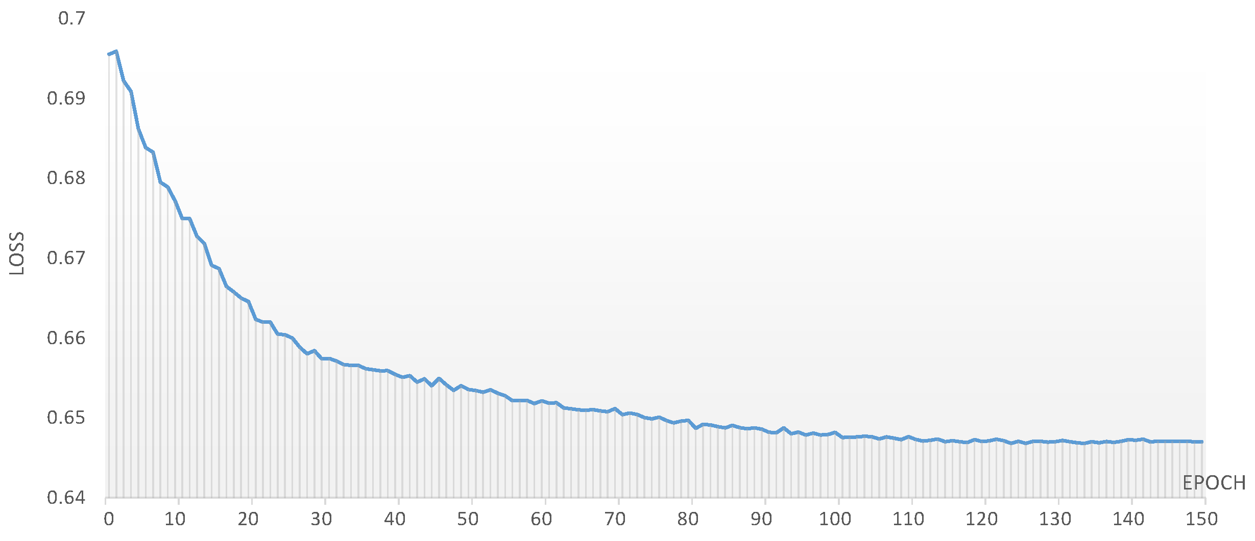
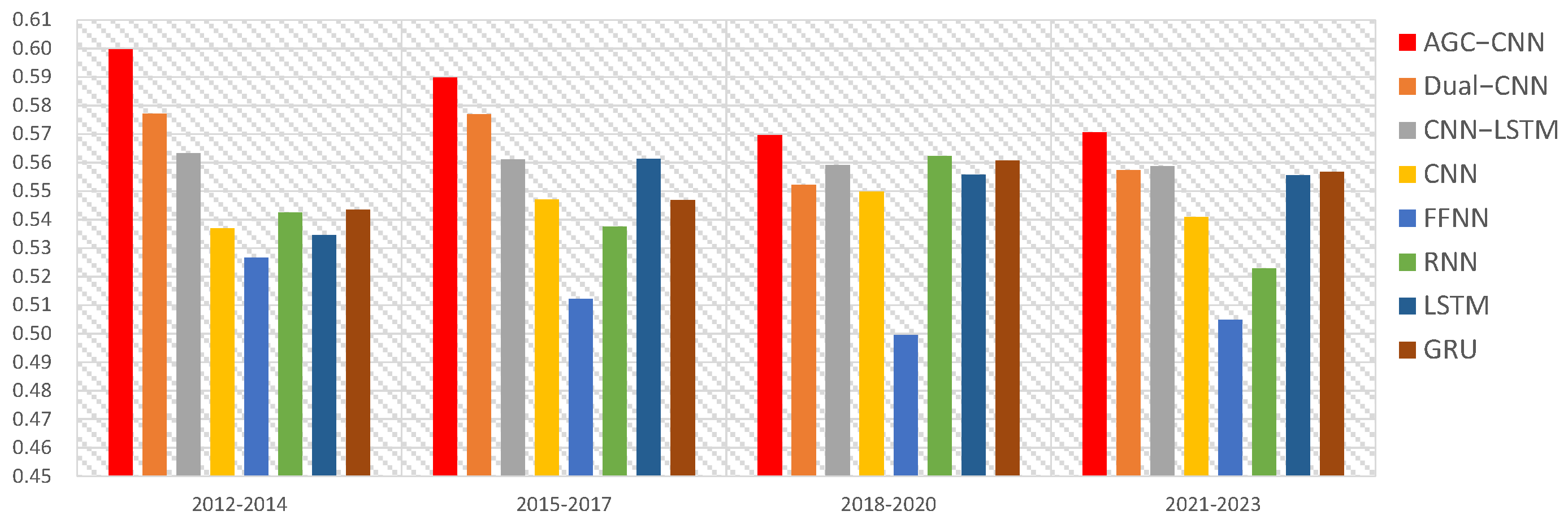
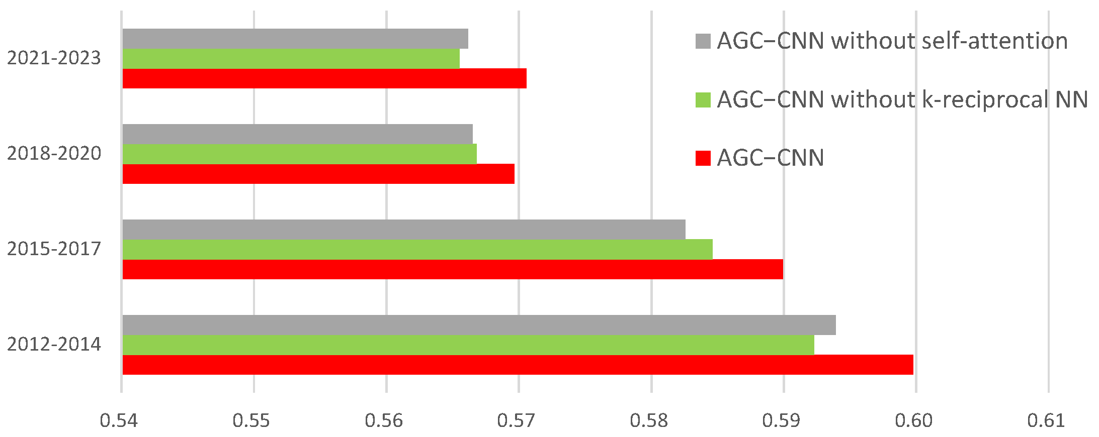
In this paper, we conducted experimental analyses over three distinct time periods, specifically from 1 January 2011 to 31 December 2023, at three-year intervals. Figure 10 illustrates the loss function of the AGC-CNN model, while Table 3 reports the accuracy of different stock trend prediction models, with its visualization illustrated in Figure 11. Figure 12 displays the accuracy of the ablation study.
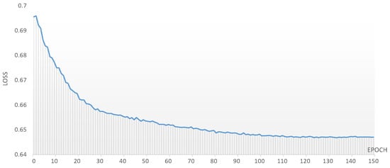
Figure 10.
The loss of AGC-CNN stock trend prediction model.

Table 3.
The accuracy of different stock trend prediction models.
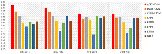
Figure 11.
The visualization of accuracy with different models.
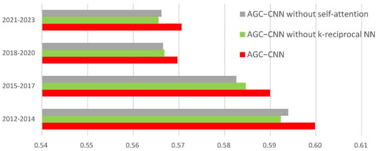
Figure 12.
The visualization of accuracy with ablation study.
It is evident that the AGC-CNN two-stage approach proposed in this paper demonstrates exceptional accuracy across all time periods, outperforming all other models under consideration. Meanwhile, the results from the ablation study (Figure 12) indicate that both the self-attention and k-reciprocal NN modules have an impact on the results, suggesting that incorporating these two modules can enhance the model’s efficiency.
The Dual-CNN model also exhibits an impressive performance throughout these periods, confirming its status as a powerful machine learning model with a stable performance. However, in contrast, the simplest form of neural network, FFNN, yields disappointing results in the experiments. Its accuracy is significantly lower than other models, failing to meet expectations. Furthermore, three different models are compared: RNN, LSTM, and GRU. The findings indicate that the performance of these three models was very close, and there is no clear winner among them. They each have their strengths in processing sequential data, but their advantages are not more prominent than the AGC-CNN and traditional CNN models. This finding further emphasizes the innovativeness and effectiveness of the AGC-CNN model presented.
5.2. The Result of Portfolio Optimization
In this section, we utilize data spanning 1 January 2012 through 31 December 2014 to train our stocks trend prediction model to identify high-quality stocks. Subsequently, we test the constructed portfolio using data from 1 January 2015 to 31 December 2015. The criterion for selecting high-quality stocks is based on how often a stock is predicted to rise in the testing set. We rank stocks in descending order according to this criterion and then select the top-k stocks. According to Remark 2, we ultimately selected 7, 8, 9, and 10 stocks, namely 7IP, 8IP, 9IP, and 10IP.
In this paper, we employed rolling window techniques, necessitating the selection of window widths. In the existing literature, window widths are typically chosen based on empirical evidence and actual data conditions, which is a commonly used method, and there is currently no established standard for selecting window widths. For instance, Kourtis et al. [42] used one month as the window width, while DeMiguel et al. [48] used 150. Ledoit and Wolf [40,50] utilized 60 and 120 as window widths, respectively. Additionally, Ledoit and Wolf [51] employed 120, 150, and 250 as window widths to verify performance stability. Therefore, we selected five rolling window widths (40, 50, 60, 70, and 80) for experimentation based on actual data conditions and empirical evidence.
Remark 2.
Regarding the issue of the number of high-quality stocks selected, Evans and Archer [52] demonstrated that the traditional rule of thumb posits that 8 to 10 stocks are adequate for optimal diversification effects. Alexeev and Dungey [53] claimed that an equally weighted portfolio of 7 (10) stocks is adequate for a typical investor seeking to diversify away 85% (90%) of the risk. Recognizing that individual investors may struggle to track too many assets, we have decided that the number of stocks we select will be between 7 and 10. This choice is tailored to accommodate the monitoring capabilities and resource limitations of individual investors while effectively diversifying the vast majority of risks.
Additionally, by assuming that investors decide to buy or sell a certain proportion of an asset prior to each trading day, we simulate the typical buying and selling behavior of investors to obtain the optimal proportions within the portfolio. We employ four criteria to measure and compare the performance of different portfolios: Cumulative Return (CR), Average Return (AR), Average Sharpe Ratio (SR), Average Turnover-adjusted Sharpe Ratio (TASR), and Average Sortino Ratio.
- (1)
- Panel A: comparison of Cumulative Return
Figure 13 displays the visualization of Cumulative Returns. From Figure 13, it is evident that, as time goes on, the AGC-CNN+GMV two-stage approach proposed in this paper has surpassed all other models. Regardless of the stock selection model used, optimizing the portfolio with the GMV model consistently outperforms the 1/N model. While other traditional models may initially perform better, their effectiveness tends to diminish over time, and they exhibit greater volatility. Additionally, the performance of AGC-CNN + MaxSR is excellent. However, since the time consumption of using MaxSR as the second-stage portfolio optimization model is 10 times that of GMV, the GMV model is preferred over MaxSR.

Figure 13.
Panel A: comparison of Cumulative Return (2015).
- (2)
- Panel B: comparison of Average Return
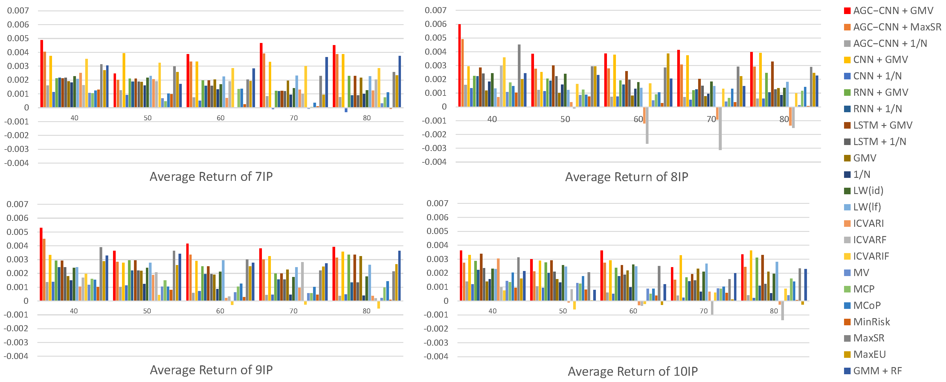
Figure 14 displays the visualization of Average Returns. From the visualization results of Average Return, it is evident that our proposed AGC-CNN+GMV two-stage approach performs the best regardless of the number of stocks selected or any other dimension considered. The performance of stock pre-selection is significantly superior to scenarios without stock pre-selection. Traditional portfolio optimization models may exhibit a better performance during certain specific periods; however, overall, their effectiveness still pales in comparison to the two-stage model we propose. Specifically, while these traditional models can yield considerable returns in individual cases, they lack the sustainability and stability of the two-stage model.
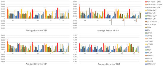
Figure 14.
Panel B: comparison of Average Return.
- (3)
- Panel C: comparison of Average SR
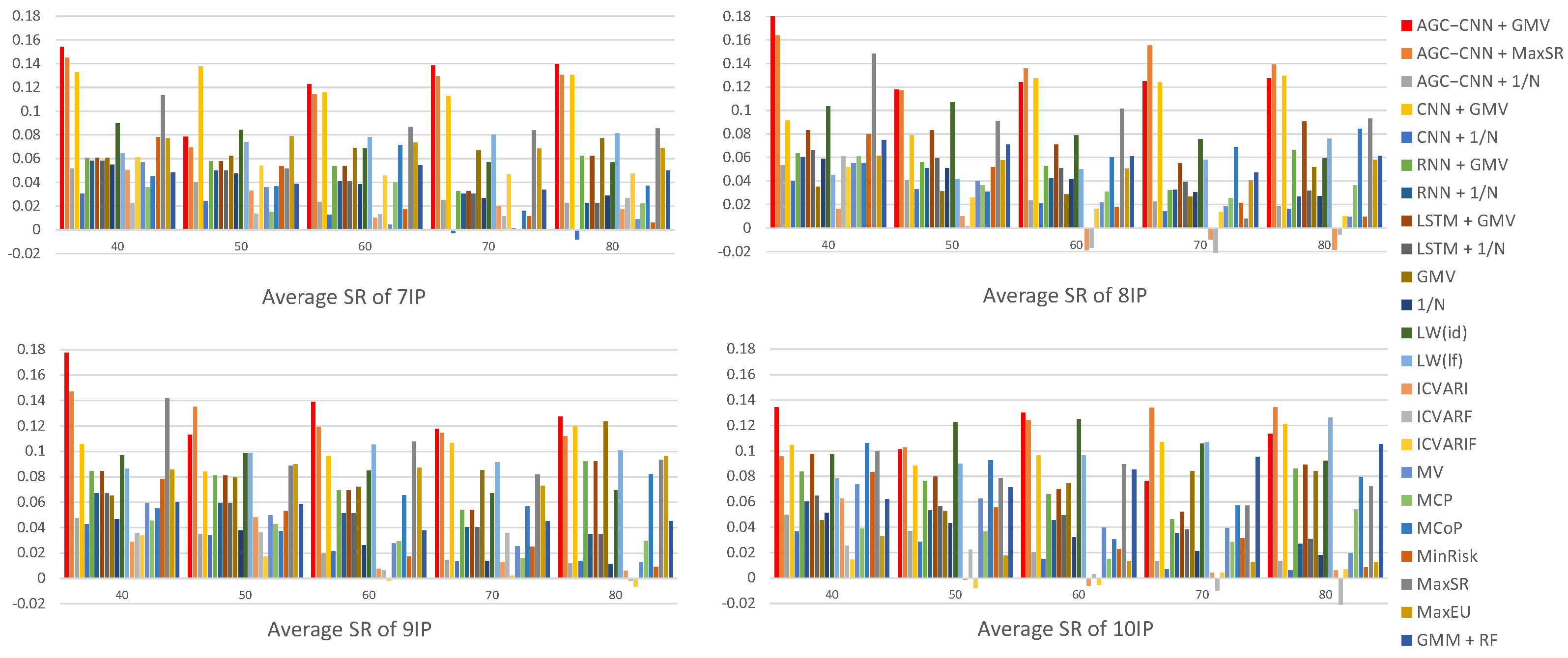
Figure 15 displays the visualization of Average SR. The visualization results of Average SR clearly show that the AGC-CNN+GMV two-stage approach has the best performance, particularly when the window width is set to 40. The average Sharpe Ratio takes into account the impact of variance, and it is evident that several traditional portfolio optimization models perform quite well, such as LW(id) and LW(lf). This indicates that some traditional models have merits in risk management, which will guide our improvements to the GMV model. Additionally, although MaxSR performs exceptionally well as the second-stage portfolio optimization model, its time consumption is significantly high.

Figure 15.
Panel C: comparison of Average SR.
- (4)
- Panel D: comparison of Average TASR
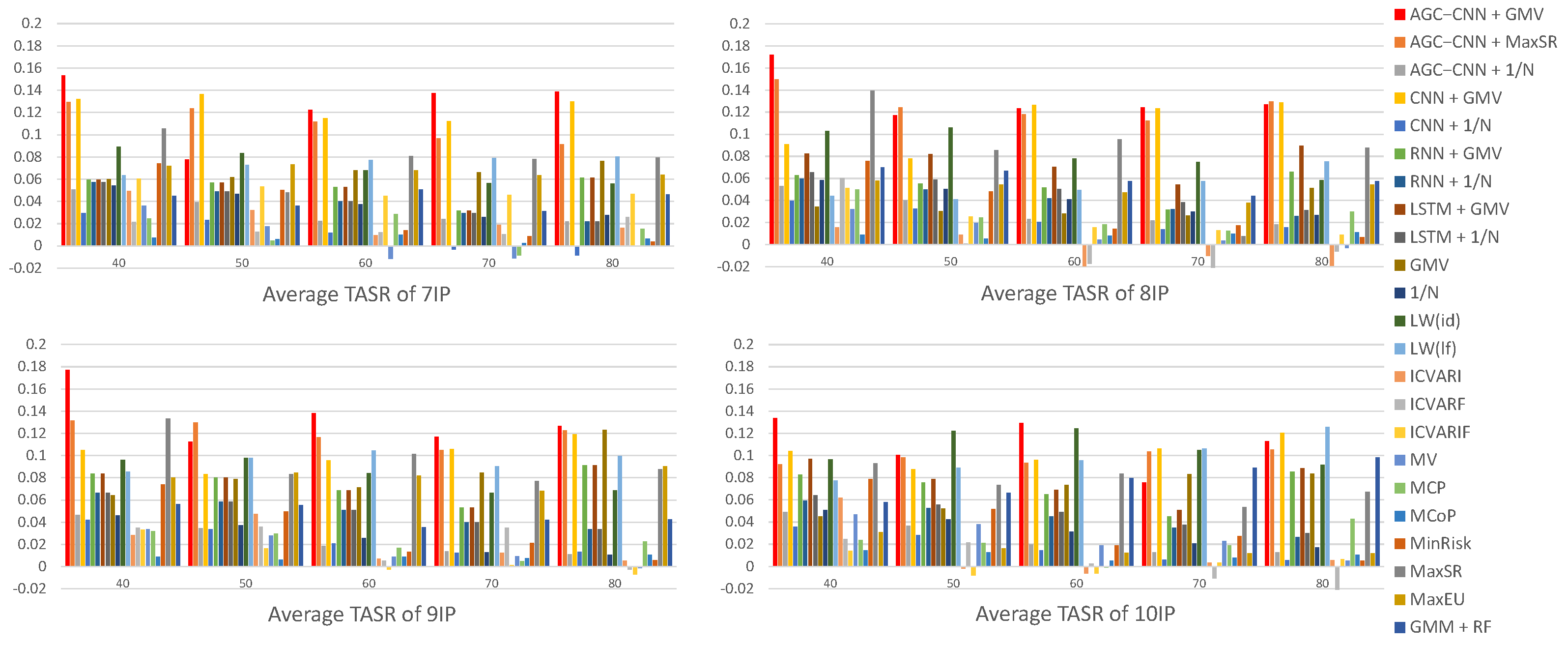
Figure 16 displays the visualization of Average TASR. The visualization results indicate that, even when considering turnover, the AGC-CNN+GMV two-stage approach proposed in this paper also exhibits excellent performance. Moreover, it can be observed that under certain conditions, the traditional portfolio optimization models can also exhibit an exceptional performance.
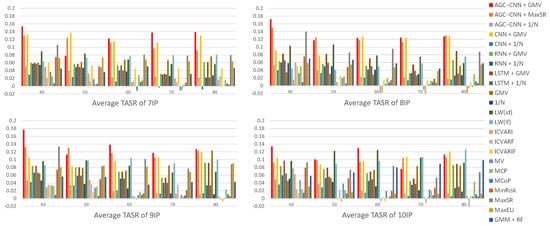
Figure 16.
Panel D: comparison of Average TASR.
- (5)
- Panel E: comparison of Average Sortino Ratio
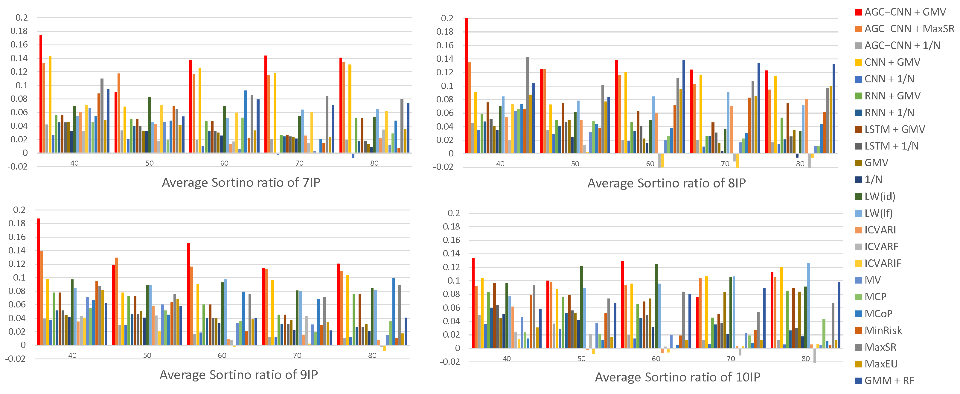
Figure 17 displays the visualization of the Average Sortino Ratio. The Sortino Ratio is a specialized measure used to evaluate investment return risks, specifically designed to focus more on downside risk—the potential loss associated with an investment—rather than overall volatility. The visualization results indicate that, when considering downside risk, the AGC-CNN+GMV two-stage approach proposed in this paper also exhibits excellent performance. Furthermore, while the traditional portfolio optimization models LW(id) and LW(lf) demonstrate commendable results during certain periods, their performance still falls short of that of the AGC-CNN+GMV model. This suggests that, although traditional models may achieve satisfactory results under specific conditions, our proposed two-stage model clearly has greater advantages in terms of overall performance and downside risk management.
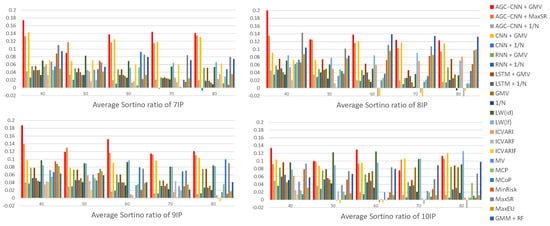
Figure 17.
Panel E: comparison of Average Sortino Ratio.
5.3. Discussion: The Effect of COVID-19 and Russia–Ukraine War
Since the emergence of the COVID-19 pandemic in December 2019 and the onset of the Russia–Ukraine war in February 2022, the global economy has faced significant challenges. To verify the effect of these events and the effectiveness of our proposed two-stage model, we performed a discussion. We employed data from 1 January 2017 to 31 December 2019 to identify high-quality stocks when subsequently leveraging data from 1 January 2020 to 31 December 2023 for portfolio optimization. To maintain the conciseness of the results, we did not use all models for validation but instead selected those that performed particularly well in the aforementioned experiments.
Figure 18 presents the visualization of Cumulative Returns from 2020 to 2023. It is evident that all models show an overall downward trend, indicating the considerable effect of the COVID-19 pandemic and the Russia–Ukraine conflict on the stock market. However, our AGC-CNN+GMV model demonstrates the most gradual decline, even showing an upward trend in 2020, highlighting the effectiveness and robustness of the model.

Figure 18.
Discussion: comparison Cumulative Return (2020–2023).
6. Conclusions
This paper introduces a novel AGC-CNN+GMV two-stage approach aimed at stock pre-selection to improve portfolio selection efficiency. In the first stage, a stock trend prediction model is proposed for stock pre-selection: the AGC-CNN model, which integrates a CNN, GCN, self-attention mechanism, and k-reciprocal NN. In the second stage, we utilize GMV to construct a portfolio selection strategy. Empirical validation of the proposed AGC-CNN+GMV two-stage approach demonstrates its effectiveness. The proposed stock trend prediction model for stock pre-selection, namely the AGC-CNN model, excels in loss performance and surpasses common deep learning models in terms of accuracy. Additionally, compared to portfolio optimization models without stock pre-selection or with other commonly deep learning models for stock pre-selection, this proposed two-stage approach achieved significant improvements in Cumulative Returns and demonstrated a robust performance in terms of Average Return, Sharpe Ratio, Turnover-adjusted Sharpe Ratio, and Sortino Ratio.
For future improvements of the proposed two-stage approach, two aspects can be considered. One aspect involves improvements to the stock trend prediction model, which can incorporate investor sentiment into consideration. Additionally, in addition to OHLC charts, other types of images can be tried for model training. The other aspect focuses on enhancements to the GMV model. Employing variances and correlations in the GMV model for portfolio selection presents certain limitations. For example, correlations fail to capture the asymmetry in correlations among different asset returns and variance lacks the ability to distinguish between higher-than-expected returns and lower-than-expected fluctuations, which impact the efficacy of portfolio selection.
Author Contributions
Conceptualization, S.H.; Methodology, S.H., L.C. and R.S.; Software, L.C.; Validation, S.H., L.C. and R.S.; Formal analysis, S.H., L.C. and R.S.; Investigation, L.C.; Resources, S.H. and R.S.; Data curation, L.C.; Writing—original draft, L.C.; Writing—review & editing, T.M. and S.L.; Visualization, L.C. and R.S.; Supervision, T.M. and S.L.; Project administration, R.S.; Funding acquisition, R.S. All authors have read and agreed to the published version of the manuscript.
Funding
This work was supported by the National Natural Science Foundation of China (grant no. 12201579).
Data Availability Statement
Data are contained within the article.
Acknowledgments
We express our sincere gratitude to the reviewers and editors for their constructive comments and valuable insights, which significantly contributed to enhancing the presentation of the manuscript.
Conflicts of Interest
The authors declare no conflicts of interest.
References
- Markowitz, H. Portfolio selection. J. Financ. 1952, 7, 77–91. [Google Scholar] [CrossRef]
- Bodnar, T.; Mazur, S.; Okhrin, Y. Bayesian estimation of the global minimum variance portfolio. Eur. J. Oper. Res. 2017, 256, 292–307. [Google Scholar] [CrossRef]
- Zhou, Z.; Gao, M.; Xiao, H. Big data and portfolio optimization: A novel approach integrating DEA with multiple data sources. Omega 2021, 104, 102479. [Google Scholar] [CrossRef]
- Wang, W.; Li, W.; Zhang, N.; Liu, K. Portfolio formation with pre-selection using deep learning from long-term financial data. Expert Syst. Appl. 2020, 143, 113042. [Google Scholar] [CrossRef]
- Bodnar, O.; Bodnar, T.; Parolya, N. Recent advances in shrinkage-based high-dimensional inference. J. Multivar. Anal. 2022, 188, 104826. [Google Scholar] [CrossRef]
- Holgersson, T.; Karlsson, P.; Stephan, A. A risk perspective of estimating portfolio weights of the global minimum-variance portfolio. AStA Adv. Stat. Anal. 2020, 104, 59–80. [Google Scholar] [CrossRef]
- Yang, F.; Chen, Z.; Li, J.; Tang, L. A novel hybrid stock selection method with stock prediction. Appl. Soft Comput. 2019, 80, 820–831. [Google Scholar] [CrossRef]
- Chen, M.; Chen, B. A hybrid fuzzy time series model based on granular computing for stock price forecasting. Inf. Sci. 2015, 294, 227–240. [Google Scholar] [CrossRef]
- Jiang, M.; Jia, L.; Chen, Z.; Chen, W. The two-stage machine learning ensemble models for stock price prediction by combining mode decomposition, extreme learning machine and improved harmony search algorithm. Ann. Oper. Res. 2020, 309, 553–585. [Google Scholar] [CrossRef]
- Cagliero, L.; Garza, P.; Attanasio, G.; Baralis, E. Training ensembles of faceted classification models for quantitative stock trading. Computing 2020, 102, 1213–1225. [Google Scholar] [CrossRef]
- Tang, H.; Dong, P.; Shi, Y. A new approach of integrating piecewise linear representation and weighted support vector machine for forecasting stock turning points. Appl. Soft. Comput. 2019, 78, 685–696. [Google Scholar] [CrossRef]
- Song, X.; Mitnitski, A.; Cox, J.; Rockwood, K. Comparison of machine learning techniques with classical statistical models in predicting health outcomes. Stud. Health Technol. Inform. 2004, 107, 736–740. [Google Scholar]
- Boulesteix, A.; Schmid, M. Machine learning versus statistical modeling. Biom. J. 2014, 56, 588–593. [Google Scholar] [CrossRef]
- Haan, L.; Mercadier, C.; Zhou, C. Adapting extreme value statistics to financial time series: Dealing with bias and serial dependence. Financ. Stoch. 2016, 20, 321–354. [Google Scholar] [CrossRef]
- Zhao, J.; Zeng, D.; Liang, S.; Kang, H.; Liu, Q. Prediction model for stock price trend based on recurrent neural network. J. Ambient Intell. Humaniz. Comput. 2021, 12, 745–753. [Google Scholar] [CrossRef]
- Sezer, O.; Ozbayoglu, A. Algorithmic financial trading with deep convolutional neural networks: Time series to image conversion approach. Appl. Soft. Comput. 2018, 70, 525–538. [Google Scholar] [CrossRef]
- Ma, W.; Hong, Y.; Song, Y. On Stock Volatility Forecasting under Mixed-Frequency Data Based on Hybrid RR-MIDAS and CNN-LSTM Models. Mathematics 2024, 12, 1538. [Google Scholar] [CrossRef]
- Nelson, D.; Pereira, A.; Oliveira, R. Stock market’s price movement prediction with LSTM neural networks. In Proceedings of the 2017 International Joint Conference on Neural Networks (IJCNN), Anchorage, AK, USA, 14–19 May 2017; pp. 1419–1426. [Google Scholar]
- Mu, S.; Liu, B.; Gu, J.; Lien, C.; Nadia, N. Research on Stock Index Prediction Based on the Spatiotemporal Attention BiLSTM Model. Mathematics 2024, 12, 2812. [Google Scholar] [CrossRef]
- Selvin, S.; Vinayakumar, R.; Gopalakrishnan, E.; Menon, V.; Soman, K. Stock price prediction using LSTM, RNN and CNN-sliding window model. In Proceedings of the 2017 International Conference on Advances in Computing, Communications and Informatics, Udupi, India, 13–16 September 2017; pp. 1643–1647. [Google Scholar]
- Wu, J.; Li, Z.; Herencsar, N.; Vo, B.; Lin, J. A graph-based CNN-LSTM stock price prediction algorithm with leading indicators. Multimed. Syst. 2021, 29, 1–20. [Google Scholar] [CrossRef]
- Jiang, J.; Kelly, B.; Xiu, D. (Re-)Imag(in)ing Price Trends. J. Financ. 2023, 78, 3193–3249. [Google Scholar] [CrossRef]
- Zhou, J.; Cui, G.; Zhang, Z.; Yang, C.; Liu, Z.; Sun, M. Graph neural networks: A review of methods and applications. AI Open 2020, 1, 57–81. [Google Scholar] [CrossRef]
- Zhang, Q.; Chang, J.; Meng, G.; Xu, S.; Xiang, S.; Pan, C. Learning graph structure via graph convolutional networks. Pattern Recognit. 2019, 95, 308–318. [Google Scholar] [CrossRef]
- Kipf, T.; Welling, M. Semi-supervised classification with graph convolutional networks. Neural Process. Lett. 2016, 54, 2645–2656. [Google Scholar]
- Wang, C.; Liang, H.; Wang, B.; Cui, X.; Xu, Y. MG-Conv: A spatiotemporal multi-graph convolutional neural network for stock market index trend prediction. Comput. Electr. Eng. 2022, 103, 108285. [Google Scholar] [CrossRef]
- Li, W.; Bao, R.; Harimoto, K.; Chen, D.; Xu, J.; Su, Q. Modeling the stock relation with graph network for overnight stock movement prediction. In Proceedings of the Twenty-Ninth International Conference on International Joint Conferences on Artificial Intelligence, Yokohama, Japan, 11–17 July 2021; pp. 4541–4547. [Google Scholar]
- Vaswani, A.; Shazeer, N.; Parmar, N.; Uszkoreit, J.; Jones, L.; Gomez, A.; Kaiser, L.; Polosukhin, I. Attention is All you Need. arXiv 2017, arXiv:1706.03762. [Google Scholar]
- Xu, H.; Chai, L.; Luo, Z.; Li, S. Stock movement predictive network via incorporative attention mechanisms based on tweet and historical prices. Neural Comput. 2020, 418, 326–339. [Google Scholar] [CrossRef]
- Lei, Z.; Zhang, C.; Xu, Y.; Li, X. DR-GAT: Dynamic routing graph attention network for stock recommendation. Inf. Sci. 2021, 654, 119833. [Google Scholar] [CrossRef]
- Li, Y.; Lv, S.; Liu, X.; Zhang, Q. Incorporating Transformers and Attention Networks for Stock Movement Prediction. J. Complex. 2022, 1076–2787. [Google Scholar] [CrossRef]
- Wang, Z.; Huang, B.; Tu, S.; Zhang, K.; Xu, L. DeepTrader: A Deep Reinforcement Learning Approach for Risk-Return Balanced Portfolio Management with Market Conditions Embedding. In Proceedings of the Twenty-Ninth International Conference on International Joint Conferences on Artificial Intelligence, Yokohama, Japan, 11–17 July 2021; pp. 643–650. [Google Scholar]
- Jegou, H.; Harzallah, H.; Schmid, C. A contextual dissimilarity measure for accurate and efficient image search. In Proceedings of the 2007 IEEE Conference on Computer Vision and Pattern Recognition, Minneapolis, MN, USA, 17–22 June 2007; pp. 9–16. [Google Scholar]
- Qin, D.; Gammeter, S.; Bossard, L.; Quack, T.; Gool, L. Hello neighbor: Accurate object retrieval with k-reciprocal nearest neighbors. In Proceedings of the IEEE Computer Society Conference on Computer Vision and Pattern Recognition, Colorado Springs, CO, USA, 20–25 June 2011; pp. 777–784. [Google Scholar]
- Bian, Z.; Liao, Y.; O’Neill, M.; Shi, J.; Zhang, X. Large-scale minimum variance portfolio allocation using double regularization. J. Econ. Dyn. Control 2020, 116, 103939. [Google Scholar] [CrossRef]
- Hoang, T. Active portfolio management for the emerging and frontier markets: The use of multivariate time series forecasts. Cogent Econ. Financ. 2022, 10, 2114163. [Google Scholar] [CrossRef]
- Maas, L.A.; Awni, Y.; Andrew, Y. Rectifier nonlinearities improve neural network acoustic models. In Proceedings of the International Conference on International Conference on Machine Learning, Atlanta, GA, USA, 16–21 June 2013; Volume 30. [Google Scholar]
- Yang, L.; Zhang, Z.; Xiong, S.; Wei, L.; Ng, J.; Xu, L.; Dong, R. Explainable text-driven neural network for stock prediction. In Proceedings of the 2018 5th IEEE International Conference on Cloud Computing and Intelligence Systems, Nanjing, China, 23–25 November 2018; pp. 441–445. [Google Scholar]
- Fischer, T.; Krauss, C. Deep learning with long short-term memory networks for financial market predictions. Eur. J. Oper. Res. 2018, 270, 654–669. [Google Scholar] [CrossRef]
- Ledoit, O.; Wolf, M. Improved estimation of the covariance matrix of stock returns with an application to portfolio selection. J. Empir. Financ. 2003, 10, 603–621. [Google Scholar] [CrossRef]
- Ledoit, O.; Wolf, M. A well-conditioned estimator for large-dimensional covariance matrices. J. Multivar. Anal. 2004, 88, 365–411. [Google Scholar] [CrossRef]
- Kourtis, A.; Dotsis, G.; Markellos, R. Parameter uncertainty in portfolio selection: Shrinkage the inverse covariance matrix. J. Bank. Financ. 2012, 36, 2522–2531. [Google Scholar] [CrossRef]
- Christoffersen, P.; Errunza, V.; Jacobs, K.; Jin, X. Correlation Dynamics And International Diversification Benefits. Int. J. Forecast. 2014, 30, 807–824. [Google Scholar] [CrossRef]
- Broadstock, D.; Chatziantoniou, I.; Gabauer, D. Minimum Connectedness Portfolios and the Market for Green Bonds: Advocating Socially Responsible Investment (SRI) Activity. In Applications in Energy Finance; Springer: Berlin/Heidelberg, Germany, 2002; pp. 217–253. [Google Scholar] [CrossRef]
- Cheng, T.; Chen, K. A general framework for portfolio construction based on generative models of asset returns. J. Finance Data Sci. 2023, 9, 100113. [Google Scholar] [CrossRef]
- Rapoport, A. Minimization of risk and maximization of expected utility in multistage betting games. Acta Psychol. 1970, 34, 375–386. [Google Scholar] [CrossRef]
- Palma, G.; Skoczeń, M.; Maguire, P. Combining supervised and unsupervised learning methods to predict financial market movements. arXiv 2024, arXiv:2409.03762. [Google Scholar]
- DeMiguel, V.; Garlappi, L.; Nogales, F.; Uppal, R. A generalized approach to portfolio optimization: Improving performance by constraining portfolio norms. Manage. Sci. 2009, 55, 798–812. [Google Scholar] [CrossRef]
- Lan, W.; Wang, H.; Tsai, C. A Bayesian information criterion for portfolio selection. Comput. Stat. Data Anal. 2012, 56, 88–99. [Google Scholar] [CrossRef]
- Ledoit, O.; Wolf, M. Robust performance hypothesis testing with the Sharpe ratio. J. Empir. Financ. 2008, 15, 850–859. [Google Scholar] [CrossRef]
- Ledoit, O.; Wolf, M. Nonlinear shrinkage of the covariance matrix for portfolio selection: Markowitz meets Goldilocks. Rev. Financ. Stud. 2017, 30, 4349–4388. [Google Scholar] [CrossRef]
- Evans, J.; Archer, S. Diversification and the reduction of dispersion: An empirical analysis. J. Financ. 1968, 23, 761–767. [Google Scholar] [CrossRef]
- Alexeev, V.; Dungey, M. Equity portfolio diversification with high-frequency data. Quant. Financ. 2015, 15, 1205–1215. [Google Scholar] [CrossRef]
Disclaimer/Publisher’s Note: The statements, opinions and data contained in all publications are solely those of the individual author(s) and contributor(s) and not of MDPI and/or the editor(s). MDPI and/or the editor(s) disclaim responsibility for any injury to people or property resulting from any ideas, methods, instructions or products referred to in the content. |
© 2024 by the authors. Licensee MDPI, Basel, Switzerland. This article is an open access article distributed under the terms and conditions of the Creative Commons Attribution (CC BY) license (https://creativecommons.org/licenses/by/4.0/).

