Abstract
With the rapid advancement of information technology, digital images such as medical images, grayscale images, and color images are widely used, stored, and transmitted. Therefore, protecting this type of information is a critical challenge. Meanwhile, quaternions enable image encryption algorithm (IEA) to be more secure by providing a higher-dimensional mathematical system. Therefore, considering the importance of IEA and quaternions, this paper explores the global exponential synchronization (GES) problem for a class of quaternion-valued neural networks (QVNNs) with discrete time-varying delays. By using Hamilton’s multiplication rules, we first decompose the original QVNNs into equivalent four real-valued neural networks (RVNNs), which avoids non-commutativity difficulties of quaternions. This decomposition method allows the original QVNNs to be studied using their equivalent RVNNs. Then, by utilizing Lyapunov functions and the matrix measure method (MMM), some new sufficient conditions for GES of QVNNs under designed control are derived. In addition, the original QVNNs are examined using the non-decomposition method, and corresponding GES criteria are derived. Furthermore, this paper presents novel results and new insights into GES of QVNNs. Finally, two numerical verifications with simulation results are given to verify the feasibility of the obtained criteria. Based on the considered master–slave QVNNs, a new IEA for color images Mandrill (256 × 256), Lion (512 × 512), Peppers (1024 × 1024) is proposed. In addition, the effectiveness of the proposed IEA is verified by various experimental analysis. The experiment results show that the algorithm has good correlation coefficients (CCs), information entropy (IE) with an average of 7.9988, number of pixels change rate (NPCR) with average of 99.6080%, and unified averaged changed intensity (UACI) with average of 33.4589%; this indicates the efficacy of the proposed IEAs.
Keywords:
quaternion-valued neural networks; global exponential synchronization; Lyapunov functions; matrix measure method; time-varying delays; image encryption MSC:
11R52; 34C28; 34D06; 92B20
1. Introduction
Recently, artificial intelligence has gained significant attention among researchers because of its broad uses across scientific and engineering disciplines. Due to these applications, many nonlinear properties of artificial intelligence have been extensively studied, including neural networks (NNs) [1,2,3]. Recently, various NNs have received significant interest primarily due to their versatile applications in diverse areas, including optimization, signal and image problems, solving nonlinear dynamical problems, and pattern recognition [4,5,6]. Consequently, many interesting and insightful results concerning NN dynamics, including stability and synchronization analysis, have been published by employing Lyapunov functions and linear matrix inequalities [7,8,9].
As we all know, RVNNs as well as complex-valued neural networks (CVNNs) have been studied extensively due to their vast application in automatic control, parallel computing problems, signal- and image-related problems, speech recognition problems, computer vision, and other fields [3,4,5,10,11,12]. However, RVNNs and CVNNs have certain limitations, especially when dealing with high-dimensional data like color images, 3D and 4D signals, medical imaging, and so on [13,14,15]. Meanwhile, researchers have found that QVNNs can overcome a wide range of issues that RVNNs and CVNNs are not able to handle because they are generalizations of RVNNs as well as CVNNs [16,17,18]. In modern engineering, QVNNs have more advantages than RVNNs and CVNNs, allowing them to be widely applicable in aerospace, satellite tracking, and magnetic resonance imaging. More specifically, quaternions allow for efficient and compact representation of three-dimensional geometric affine transformations. Due to these various applications, researchers have developed QVNNs by utilizing the properties of quaternions. As a result, QVNNs have become a powerful modeling tool and have attracted growing attention from researchers. Recently, numerous researchers have explored QVNNs in greater depth, uncovering many significant findings [19,20,21]. Additionally, most recent research has concentrated on studying dynamical properties of NNs, including stability [3], periodic solutions [6], and bifurcation analysis [9]. While considering the dynamics of NNs, synchronization is essential, ensuring that neurons exhibit the same dynamical behavior simultaneously, enabling the NNs to respond quickly and exactly. In absence of synchronization, neurons may lead to undesirable results [22]. Thus, considering synchronization in NNs is essential for theoretical as well as practical perspectives. Recently, a huge number of synchronization issues have been studied vastly, especially due to their broad uses, such as secure communications, image- and signal-related problems, and biological systems [23,24,25].
Moreover, due to limitations in transmission speed and network bandwidth, time delays are inevitably introduced, which can significantly reduce network performance and compromise stability. This adds complexity to both the theoretical analysis and practical application of NNs. Hence, it is crucial to study time delays’ influence on network dynamics [26,27,28]. Recently, various methods to address time delays have been extensively studied to enhance our understanding of NN dynamics [3,6,8,24,26,27]. On the other hand, multiple approaches, including the MMM, have been applied to analyze NN dynamics. MMM has recently gained popularity for its precision in handling connection weights that include both positive and negative values. Additionally, MMM is highly sensitive and eliminates the need for complex Lyapunov function construction, ensuring results obtained from MMM are more precise and less conservative when compared to those derived from matrix norms. Consequently, MMM has been widely used to examine the dynamics of RVNNs and CVNNs [29,30,31,32,33]. On the other hand, image encryption technology is applicable across numerous domains for protecting sensitive visual data. In healthcare, encrypted medical images ensure patient anonymity during data exchange between hospitals. Moreover, in military operations, encrypted satellite imagery might obstruct adversaries from obtaining vital intelligence. In recent years, IEAs employing chaotic systems have attracted considerable attention from researchers. However, existing IEAs fail to achieve an optimal equilibrium among security and efficiency. To address the limitations of existing algorithms, an IEA employing chaotic systems has attracted considerable attention from scholars. Several different algorithms for encrypting images have been proposed [34,35,36,37,38,39,40]. According to the author’s knowledge, MMM has not been used to examine the GES of QVNNs with non-differentiable discrete time-varying delays through decomposition and non-decomposition methods. Furthermore, the synchronization criteria derived have not been applied to color IEAs. This makes the current work both necessary and valuable for further investigation.
Motivated based on the foregoing discussion, we shall investigate the GES for the class of QVNNs incorporating non-differentiable time-varying delays. Inspired based on the studies in [30,33], by utilizing suitable Lyapunov functions as well as the Halanay inequality, new matrix-measure-based GES criteria for considered QVNNs under designed control are obtained. Also, this paper presents novel results as well as new insights to achieve GES of QVNNs. We conclude by illustrating the feasibility of the obtained synchronization criteria through two numerical examples. As compared to some previous results, this paper has the following significant advantages: (i) For the first time, we employ MMM to investigate the GES for QVNNs with non-differentiable time-varying delays via decomposition and non-decomposition methods; (ii) By utilizing MMM, we obtain several sufficient criteria for the GES of QVNNs, which provides results that are more precise than those obtained using matrix norms; (iii) By using master–slave QVNNs, a new IEA for color images is proposed including different security measures to analyze the performance of the cipher image; (iv) This study presents more general results than previous studies, since they remain valid even when the considered QVNNs are reduced to RVNNs or CVNNs.
The paper follows the following structure: Section 2 presents preliminary information on quaternion algebra, the problem model, activation functions, and time delays. Section 3 provides useful definitions, lemmas, and the main results of the paper: Theorem (1) and Corollary (1) offer GES criteria based on the decomposition method, while Theorem (2) presents GES criteria using the non-decomposition method. Section 4 includes two numerical examples to demonstrate the feasibility of the main results. Section 5 applies the theoretical findings to color image encryption. Finally, Section 6 concludes the paper.
2. Problem Formulation and Preliminaries
2.1. Notations
, , and represent the sets of all real numbers, complex numbers, and quaternions. represents the n-dimensional real space, represents the n-dimensional complex space and represents the n-dimensional quaternion space. , , and represent the sets of all real matrices, complex matrices, and quaternion matrices, respectively. Additionally, and represent the transpose and conjugate transpose of the matrix , respectively.
2.2. Quaternion Algebra
The quaternion is a four-dimensional vector space associated with and ordered basis consisting of 1, i, j, and k. A quaternion number can be expressed as follows: , where . The imaginary terms i, j, and k follow Hamilton’s multiplication rules, which are defined as follows: . These rules illustrate that the quaternion multiplication does not satisfy commutative property. When considering two quaternions and , their addition can be described as follows: . The product between them is defined by Hamilton’s multiplication rules as follows: . For any quaternion , the conjugate of is symbolized by , which is defined as and the norm of is defined as . More information about quaternions can be found in [13,14,15].
2.3. Problem Formulation
We examine the QVNNs with time-varying delays that are given below:
in which time ; denotes the neural state vector; , where denotes the weight matrix for self-feedback neurons; and denote the weight matrices for interconnection neurons; denotes the neuron activation; denotes the external input vector.
Assumption A1.
Assume that the discrete time-varying delay holds the following condition:
where represents a non-negative constant.
Assumption A2.
The function satisfies the Lipschitz continuity property, i.e., there is such that for any , we have
The initial state vector of (1) is given as follows:
in which is continuous on .
To investigate the synchronization behavior of QVNNs [22,33], we define the master QVNNs given in (1), while the corresponding slave QVNNs can be described as follows:
in which and represent the neural state and control input vector, separately; , and are similar to those mentioned in the QVNNs (1).
The initial state vector of (3) is given as follows:
in which is continuous on .
3. Main Results
Here, we derive matrix-measure-based GES criteria for the master–slave QVNNs (1) and (3) based on decomposition and non-decomposition methods.
3.1. Decomposition-Method-Based Synchronization Analysis
Initially, we express the QVNNs in (1) into the following RVNNs by dividing them into their real and imaginary components:
in which , , , . We denote the real and imaginary components using the superscripts , , , and , where , , , .
The initial state of (5) is given as follows:
in which , , , , and is the norm function of , where and .
Assumption A3.
The functions , , and hold the Lipschitz continuity property, i.e., there exist , , and such that for any , we have
Correspondingly, we divide the QVNNs in (3) into their real and imaginary components as follows:
where , , , and , , , represent the control input vectors.
The initial state of (7) is given as follows:
in which , , , .
3.2. Preliminaries
Definition 1
([41,42]). For any , the real vector norm is given as follows:
Likewise, for any , where , the quaternion vector norm is given as follows:
For constant matrix , the matrix norm is defined as follows:
Likewise, for constant matrix , the matrix norm is defined as follows:
Definition 2
([41,42]). The matrix measure of a matrix is as follows:
in which denotes the matrix norm on , and is an identity matrix.
We can determine the matrix measure through simple mathematics as follows:
Definition 3
([41,42]). The matrix measure of a matrix is as follows:
in which denotes the matrix norm on , and is an identity matrix.
We can obtain the matrix measure based on simple mathematics as follows:
Lemma 1
([33,41]). As defined in Definition (2), the matrix measure includes the following:
- (1)
- ,
- (2)
- ,
- (3)
- , .
Lemma 2
([33,41]). Suppose and are constants with and a non-negative continuous function defined on the interval which satisfies, for all ,
where . Then,
in which denotes the unique solution of
and is defined as
Remark 1.
As is well known, there are notable distinctions among matrix norms and matrix measures. But matrix norms are limited because of its non-negative values, while matrix measures can provide positive as well as negative values. Additionally, MMM is sensitive to sign; specifically, in general, whereas . Due to its special properties, MMM provides many advantages over matrix norms in terms of obtaining precise results.
We have adopted the following notations in order to simplify the resulting parts: , , , , , , , , , , , , , , , , , .
The subsequent Theorem (1) derives the GES criteria between the master–slave QVNNs (5) and (7) by choosing appropriate controller gain matrix via decomposition method.
Theorem 1.
Proof.
The Lyapunov functions are defined as follows:
where
Utilizing the Dini derivation and Taylor’s theorem based on Peano’s remainder form, we can estimate the Dini derivative of along the QVNNs described in (13) as follows:
By the similar techniques, the Dini derivative of , , along the QVNNs (13) can be estimated by
The combinations of (16)–(19) deduce to
By using Assumption 3, we have
By substituting (21)–(28) into (20), we obtain
Using Definition (2) and (29), we obtain
Let
On the basis of (14), we have . It follows from Lemma (2) that
where represents the unique positive solution of
As stated in Definition (5), decays exponentially to zero with a rate of . This implies that , , , and converge globally and exponentially to zero, leading to the conclusion that the master QVNNs in (5) are GES with respect to the slave QVNNs in (7). The proof is complete. □
Corollary 1.
Proof.
Remark 2.
There are many studies on QVNN dynamics based on the decomposition method available in the literature [16,17,18]. Ultimately, the primary reason for using the decomposition method is to avoid the non-commutativity difficulties associated with quaternions, which makes it much easier to understand the analysis process and the resulting conditions. By taking these merits into account, the calculation process of Theorem (1) and Corollary (1) have been derived by employing the decomposition method, which increases the theoretical analysis complexity but greatly reduces the difficulties of analysis.
3.3. Non-Decomposition-Method-Based Synchronization Analysis
In this subsection, we will derive matrix-measure-based GES criteria for the master–slave QVNNs (1) and (3) based on the non-decomposition method.
To investigate the synchronization dynamical behavior of QVNNs, we utilize the master QVNNs described in (1) and the slave QVNNs presented in (3). Also, we consider the control input by using the linear combinations of differences among the state of master–slave QVNNs (1) and (3) as follows:
in which represents the controller gain matrix.
Here, we introduce the synchronization errors between the master–slave QVNNs (1) and (3) with the control law (37) as follows:
in which , , , .
The subsequent Theorem (2) provides the GES criteria for the master–slave QVNNs (1) and (3) by selecting on appropriate controller gain matrix via the non-decomposing method.
Theorem 2.
Proof.
The Lyapunov functions are defined as follows:
Utilizing the Dini derivation and Taylor’s theorem based on Peano’s remainder form, we can estimate the Dini derivative of along the QVNNs described in (38) as follows:
By using Assumption 2, we have
By substituting (42) and (43) into (41), we obtain
Using Definition (3) and (44), we obtain
Let , .
On the basis of (39), we have . It follows from Lemma (2)
in which represents the unique positive solution of
As stated in Definition (4), decays exponentially to zero with a rate of . This implies that converge globally and exponentially to zero, leading to the conclusion that the master QVNNs in (1) are GES with respect to the slave QVNNs in (3). The proof is complete. □
Remark 3.
As we all know, the decomposition methods lead to larger system sizes and present mathematical challenges. Moreover, the decomposition methods add complexity to theoretical analysis. Hence, the calculation process of Theorem (2) has been derived by using the non-decomposition method for the first time, which greatly reduces the mathematical challenges and complexity of theoretical analysis.
Remark 4.
There have been many studies on NN dynamics based on the Lyapunov functions available in the literature [19,21,23,24,25]. In reality, selecting the right Lyapunov functions as well as proving the stability or synchronization of NNs is a very complex process. However, by using MMM, the Lyapunov function can itself be expressed based on the matrix measures of variables or error vectors. Hence, the results obtained in this paper are more concise.
Remark 5.
Recently, several authors have examined various stability or synchronization analyses of RVNNs and CVNNs based on Lyapunov functions by applying the Halanay inequality and MMM [29,30,32,33]. To the best of our knowledge, no papers have been published pertaining to the stability or synchronization analysis of QVNNs using MMM. To fill this gap, we have examined the GES problem of QVNNs for the first time by utilizing Lyapunov functions, the Halanay inequality as well as MMM via decomposition and non-decomposition methods. Moreover, the results obtained in this paper are new as well as more general than those presented in previous studies [29,33].
Remark 6.
It is essential to note that the sufficient conditions derived from Theorem (1), (2) and Corollary (1) are independent of the time-delays but depend on the inequality of the system variables and controller gain matrix.
4. Numerical Examples
Here, we present two numerical case studies to describe the advantages and validity of our theoretical findings.
Example 1.
In master QVNNs (1), assuming , we consider
and let the two-neuron slave QVNNs be defined as follows:
Take as a discrete time-varying delay, which shows that its supremum is . Further, the activation functions are considered as . One can verify that Assumption 3 holds with , , , . Using a simple calculation, we can obtain , , , , , , , . By choosing , we can verify the condition (14) of Theorem (1) is satisfied based on the above parameters as . On the basis of Theorem (1), we can state that the master–slave QVNNs (48) and (49) achieve GES.
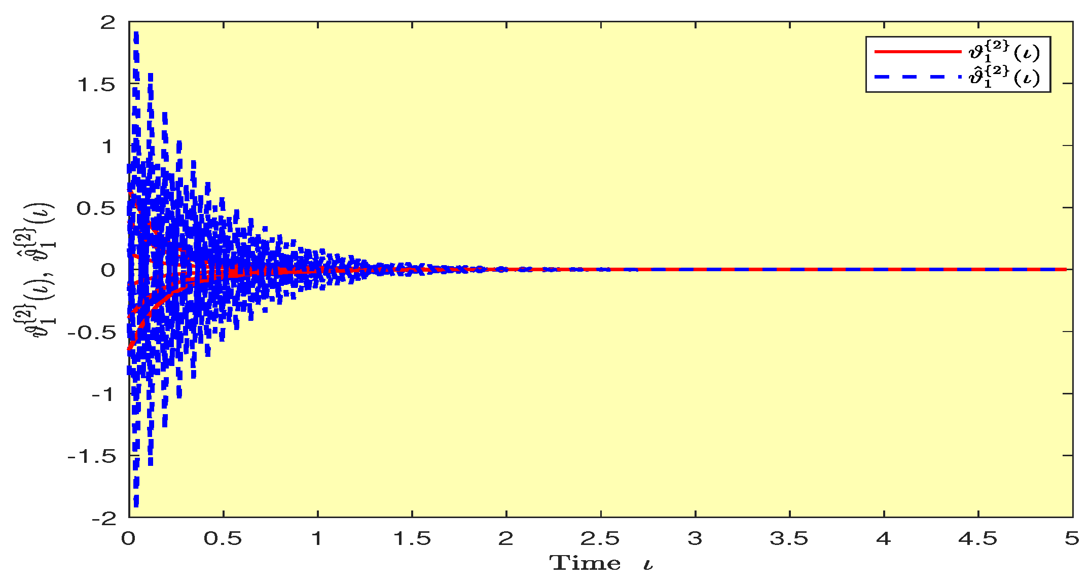
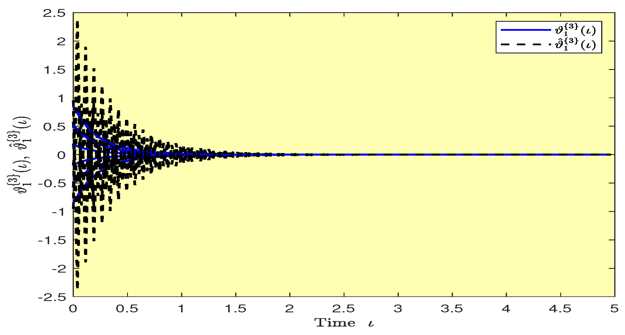
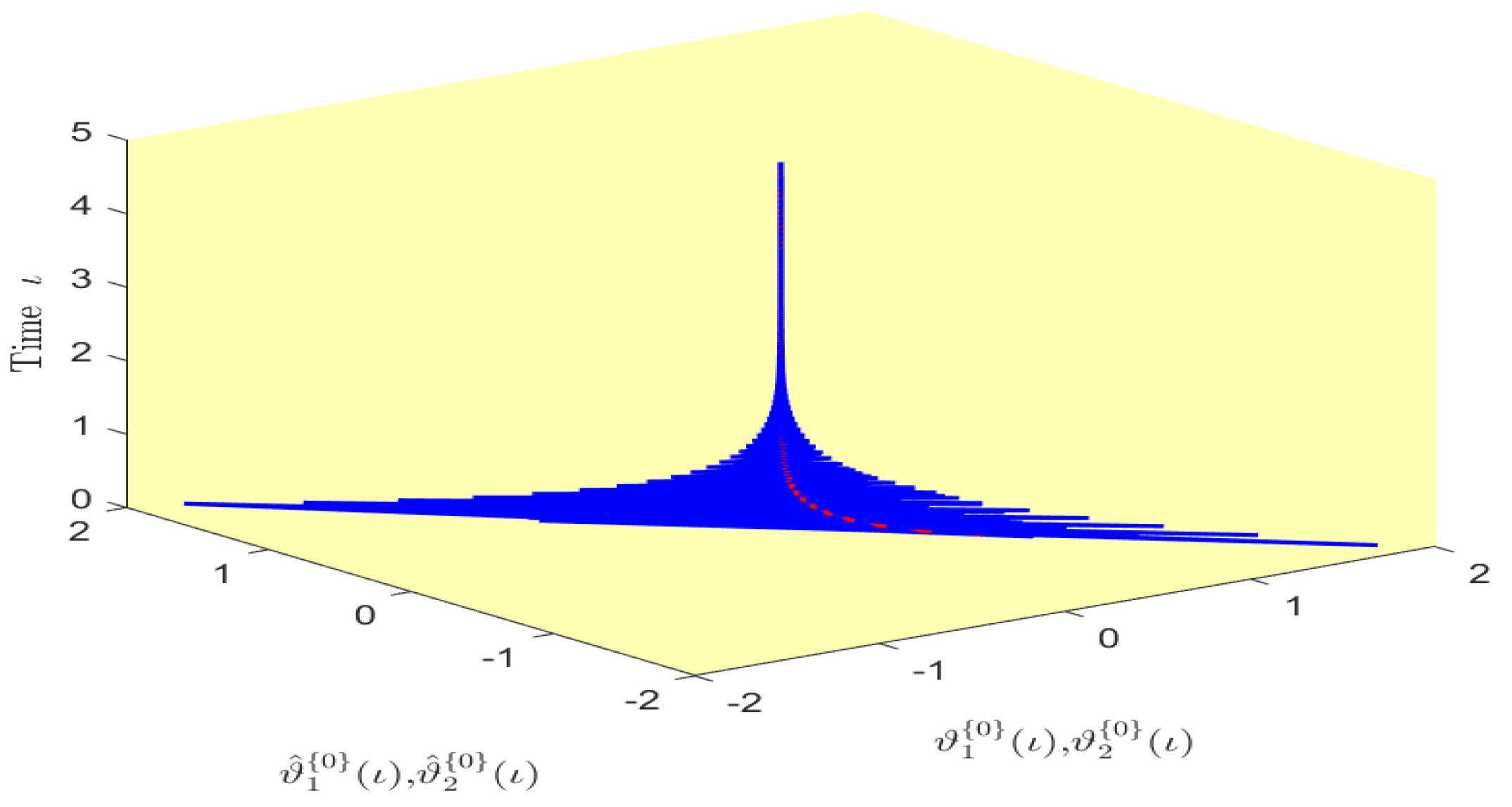
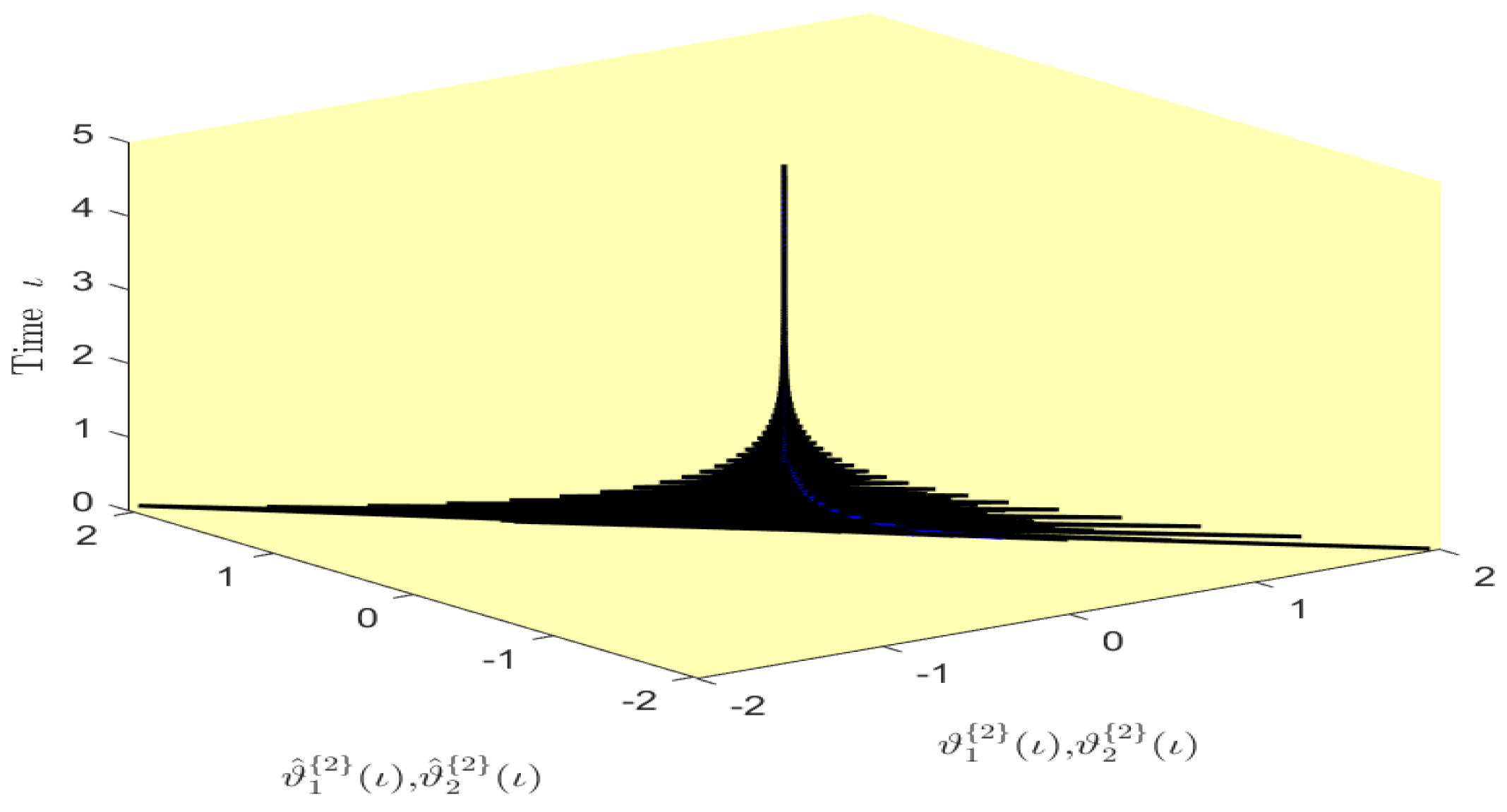
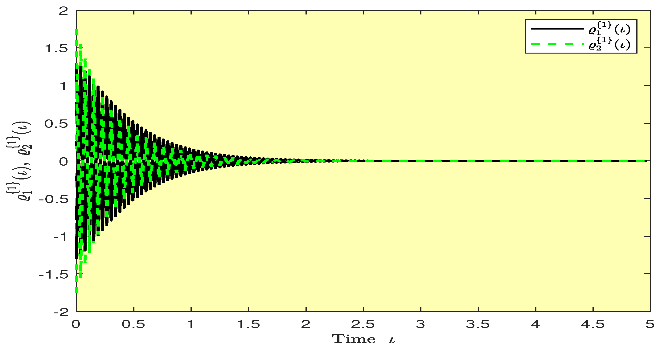
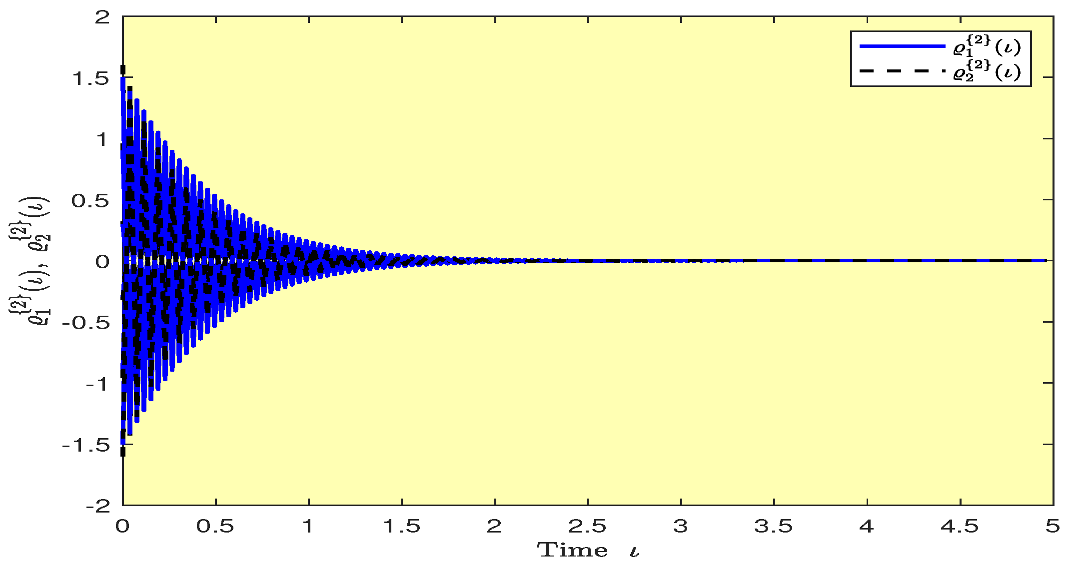
Based on randomly selected six initial conditions, the transient behaviors and phase plots of the states of master–slave QVNNs (48) and (49) are presented in Figure 1, Figure 2, Figure 3, Figure 4, Figure 5, Figure 6, Figure 7, Figure 8, Figure 9, Figure 10, Figure 11 and Figure 12. Figure 1, Figure 2, Figure 3, Figure 4, Figure 5, Figure 6, Figure 7 and Figure 8 depict the transient behaviors of the states corresponding to the real and imaginary parts. Figure 9, Figure 10, Figure 11 and Figure 12 show the phase diagrams of the states corresponding to the real and imaginary components. Figure 13, Figure 14, Figure 15 and Figure 16 depict the synchronization errors , , , , between the master–slave QVNNs (48) and (49) with control gain matrix . From these simulation results in Figure 1, Figure 2, Figure 3, Figure 4, Figure 5, Figure 6, Figure 7, Figure 8, Figure 9, Figure 10, Figure 11, Figure 12, Figure 13, Figure 14, Figure 15 and Figure 16, it is clear that the master–slave QVNNs (48) and (49) have achieved GES.
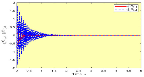
Figure 1.
Transient behaviors of the states and over time in Example 1.
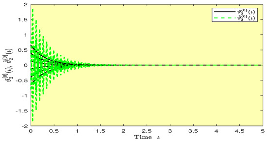
Figure 2.
Transient behaviors of the states and over time in Example 1.
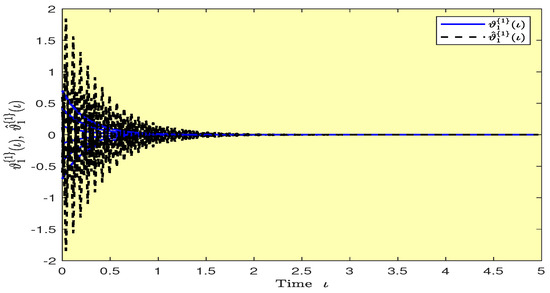
Figure 3.
Transient behaviors of the states and over time in Example 1.
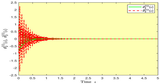
Figure 4.
Transient behaviors of the states and over time in Example 1.
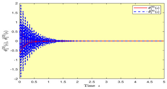
Figure 5.
Transient behaviors of the states and over time in Example 1.
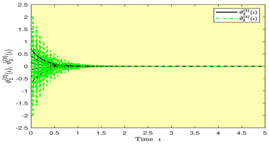
Figure 6.
Transient behaviors of the states and over time in Example 1.

Figure 7.
Transient behaviors of the states and over time in Example 1.

Figure 8.
Transient behaviors of the states and over time in Example 1.
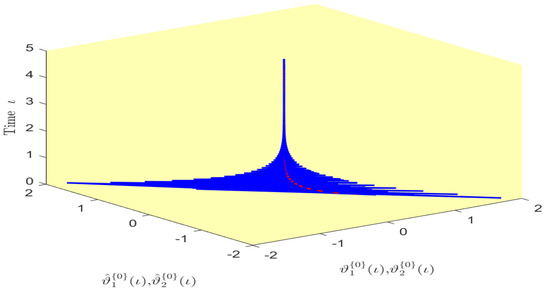
Figure 9.
Phase diagram of the states and over time in Example 1.
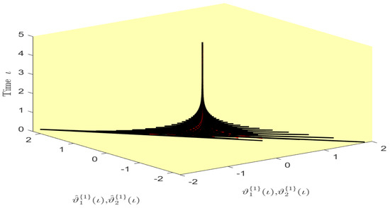
Figure 10.
Phase diagram of the states and over time in Example 1.
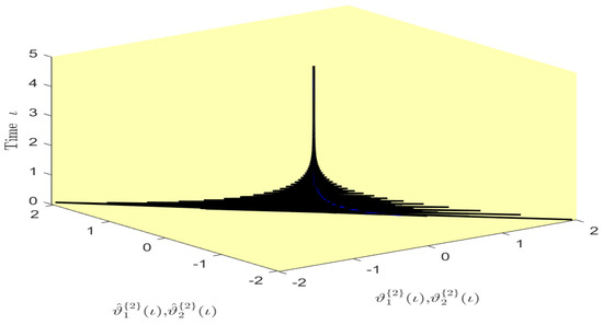
Figure 11.
Phase diagram of the states and over time in Example 1.
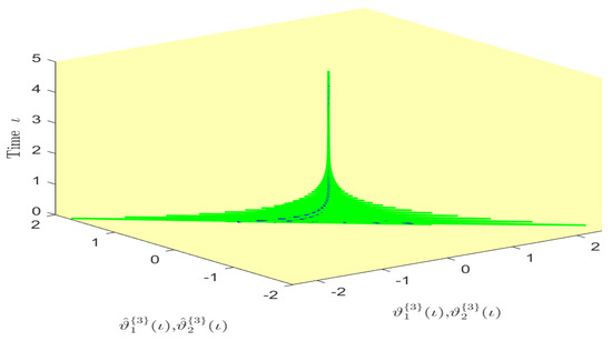
Figure 12.
Phase diagram of the states and over time in Example 1.
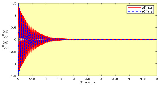
Figure 13.
Plots of the synchronization errors over time in Example 1.

Figure 14.
Plots of the synchronization errors over time in Example 1.

Figure 15.
Plots of the synchronization errors over time in Example 1.
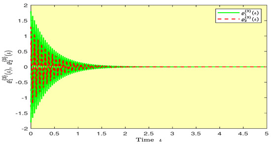
Figure 16.
Plots of the synchronization errors over time in Example 1.
Remark 7.
In [41], the authors used state coupling control to achieve GES for a class of NNs. However, the control gain matrix needs to be symmetric as well as a positive–definite matrix, which is restrictive. In contrast, the control gain matrix based on this paper has no such special requirements. So, our results are new and more general. To prove this, we utilize the same system parameters in Example 1 and select the control gain matrix as . Letting , we can verify that condition (14) of Theorem (1) is satisfied as . In addition, the control gain matrix only needs to be adjusted to satisfy the sufficient conditions presented in this paper and to achieve GES.
Example 2.
In master QVNNs (1), assuming , we consider
and let the two-neuron slave QVNNs be defined as follows:
The activation functions are considered as . It is obvious that Assumption 2 holds with . Further, the discrete time-varying delay is defined as , which shows that its supremum is . By choosing , and using the parameters above, we can easily verify that the condition (39) of Theorem (2) is satisfied with the above parameters as . By applying Theorem (2), it is clear that the master–slave QVNNs (50) and (51) are GES.
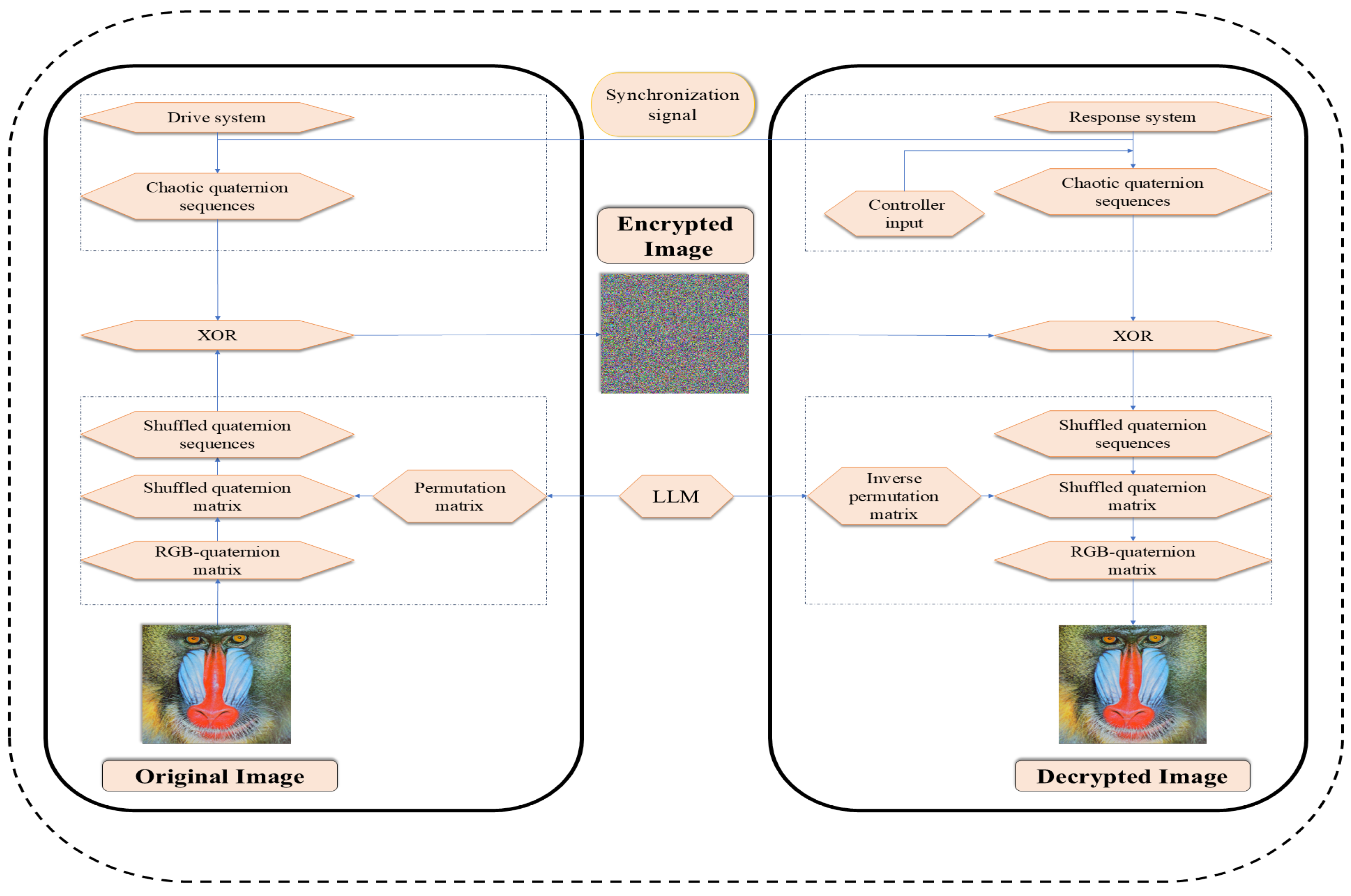
5. Application to Image Encryption
Here, we address the application of master–slave QVNNs (48) and (49) in IEA. First, a color image cryptosystem is proposed, and performance is assessed applying certain security criteria.
5.1. Background on the Color Image
Color spaces serve as a standardized method used for encoding and representing colors in a digital format, allowing images to be recorded, displayed, and manipulated accurately. This paper uses the -based color space among different color space models to analyze the color image. In the -based color space, red , green , and blue are the basic colors that is depicted by gray values with integers between 0 to 255. According to previous works [44,45], there is a one–one function from components to quaternions with imaginary components only, i.e., . Therefore, we utilize pure quaternion matrix to represents a color image with pixels, where . The pure quaternion corresponds to the color at pixel . Specifically, , where and .
5.2. Permutation Procedure
Let the dimension of the original color space color image be . Then, the original color image can be represented by a quaternion matrix , where is a pure quaternion indicating the color at the pixel of the image. Let , where . So, is the dimension of component matrix. Before encrypting, we first shuffle the original image matrix , that is, change the row and column position of matrix in a certain way. To shuffle the matrix , we need a chaotic sequence to generate the permutation square matrix of which the elements are only 0 and 1, and each row or column has one and only one 1. This permutation square matrix has the following properties:
- We can rearrange the rows of by multiplying a permutation square matrix to the left of (i.e., ). Similarly, we can rearrange the columns of by multiplying a permutation square matrix to the right of (i.e., ).
- The inverse of a permutation matrix is simply its transpose (i.e., ).
- One can obtain .
To obtain a valid permutation procedure, we utilize the following logistic–logistic map (LLM), to generate the chaotic sequence.
where is the initial value of the sequence and the parameter . As mentioned in early works [20], the LLM’s chaotic range and performance are much better than the previous logistic map’s. The generation process of the row permutation matrix is summarized as follows:
- For given initial values and , iterate the LLM (52) to obtain .
- Consider . Obviously, we have .
- Perform the iteration LLM (52) until there are unique and different values located from 1 to . Then, arrange these unique and different values in an orderly manner to be stored in , .
- For each , we have , , . After replaying the th row of the identity matrix on the th row of the row permutation matrix , we obtain the row permutation matrix . Similarly, the column permutation matrix is obtained.
For example, we choose for the row permutation matrix and . Thus, we have
In this way, the shuffled image can be obtained from the matrix as follows:
where is the shuffled image, and denotes the row permutation matrix. Also, denotes the column permutation matrix. Then, the IEA based on QVNNs with time-varying delay is proposed in the next subsection.
5.3. QVNN-Based Encryption Algorithm
The proposed synchronization method will be applied to IEA for an color image based on the size of based on QVNNs (48) and (49) as shown below:
- S1:
- Separate the channels of shuffled image into three gray ones with red, green, and blue. Hence, three new pixel matrices are obtained as , and , in which and .
- S2:
- Arrange the pixels of each , and in the order from left to right and then top to down to obtain .
- S3:
- To obtain the chaotic sequences, the master QVNN (48) is iterated continuously times with a step size of 0.001. Then, after a certain transformation, the chaotic signals can be obtained as shown in Algorithm 1. In Algorithm 1, the symbol denotes the flooring operation, whereas mod denotes the modulo operation.
- S4:
- The ciphertext can be obtained by the following operation, i.e., , where and ⊕ corresponds to the XOR operator. Then, the decryption scheme is identical to the discussed encryption scheme in reverse order, which is neglected.
| Algorithm 1: Reorganizing Chaotic Sequences. |
| Require: |
| 1. ; |
| Ensure: |
| 2. for do 1 to |
| 3. ; |
| 4. ; |
| 5. ; |
| 6. end |
5.4. Simulation Results
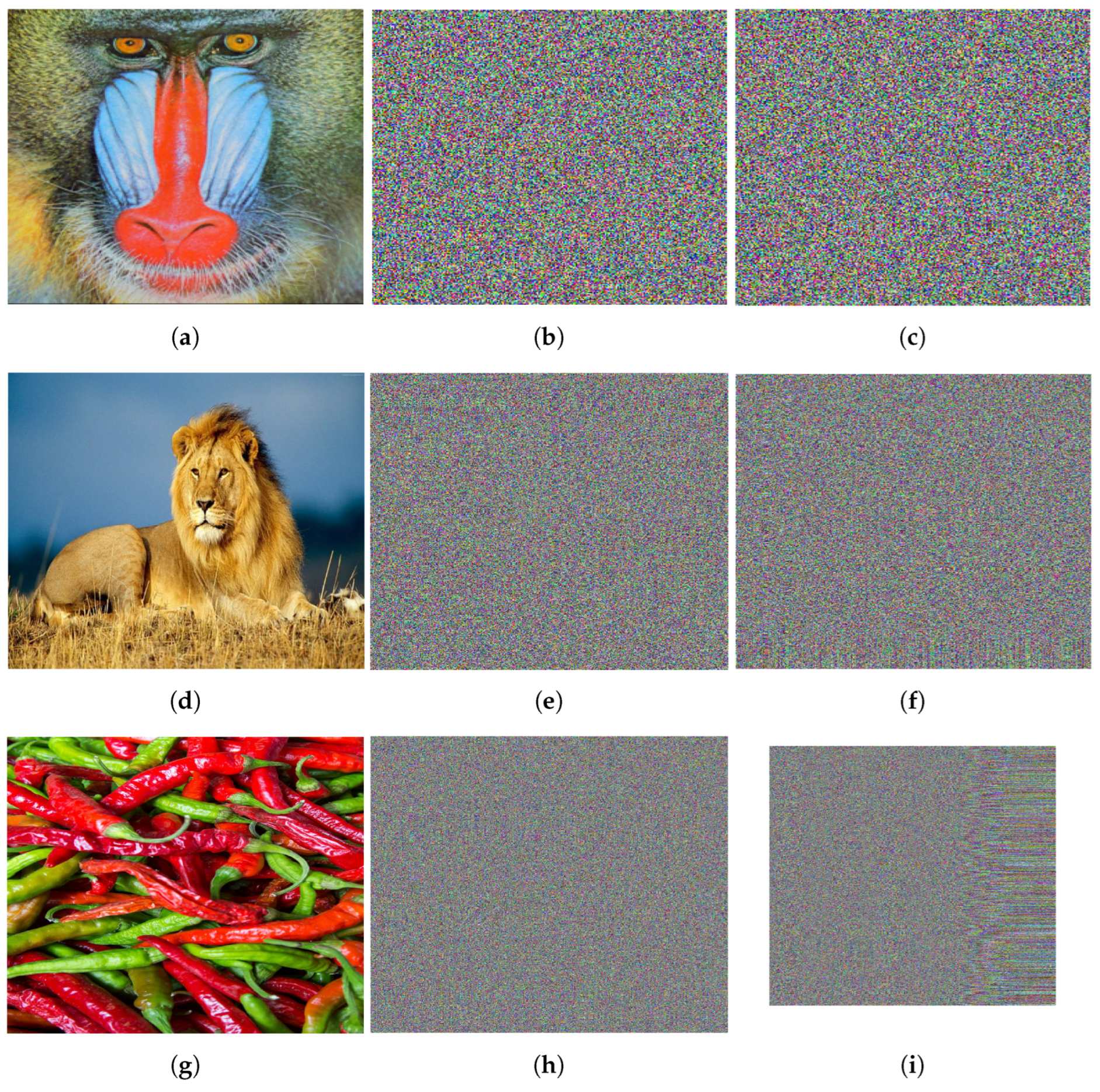
The proposed IEA is tested using MATLAB R2024a on a computer with an Intel(R) Core(TM) i7-1355U CPU @1.2 GHz 3.7 GHz, Microsoft Windows 11 Pro operating system with 32 GB memory. We choose the parameters , for the LLM (52) and the QVNN is the same as (48) in Example 2. Figure 17 shows the original, encrypted, and decrypted color images: Mandrill , Lion , and Peppers . The encryption and decryption have been implemented through the operation shown in Figure 18.
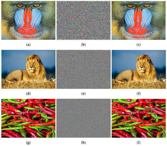
Figure 17.
(a–c) corresponds to original, encrypted, and decrypted (using correct key) images of “Mandrill”. (d–f) corresponds to original, encrypted, and decrypted (using correct key) images of “Lion”. (g–i) corresponds to original, encrypted, and decrypted (using correct key) images of “Peppers”.
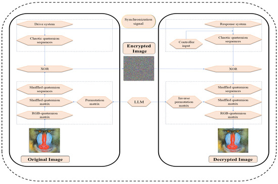
Figure 18.
The flow chart of encryption process.
5.5. Performance Analysis
In this subsection, we use various security measures to analyze the performance of our color cipher image.
5.6. Key Space Analysis
The key space represents the complete set of all permissible keys available in an IEA. The encryption keys are obtained from the QVNNs in Example 1 using the parameters , , , and initial functions. In addition, the parameters and from LLM can also be in the key space. That means the key space from this encryption scheme is huge to withhold brute-force attacks.
5.7. Key Sensitivity Analysis
Key sensitivity is based on when slight changes in the key affect the resulting decrypted image. A high level of key sensitivity is crucial for a secure IEA. A high level of key sensitivity ensures a small variation in the keys fails to decrypt the image. To analyze the key sensitivity of the encrypted scheme of this paper, we tested it using incorrect keys that were slightly different from the keys to decrypt the encrypted image, which is shown in Figure 19. As shown in Figure 19, the results indicate that, even if attackers obtain the encrypted image, recovering the original image accurately remains impossible without the correct keys. This shows the strong key sensitivity of the proposed IEA.
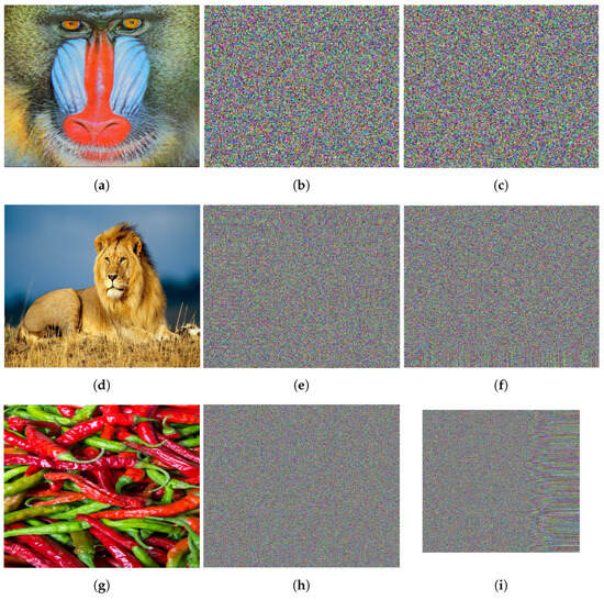
Figure 19.
(a–c) corresponds to original, encrypted, and decrypted (using wrong key) image of “Mandrill”. (d–f) corresponds to original, encrypted, and decrypted (using wrong key) image of “Lion”. (g–i) corresponds to original, encrypted, and decrypted (using wrong key) image of “Peppers”.
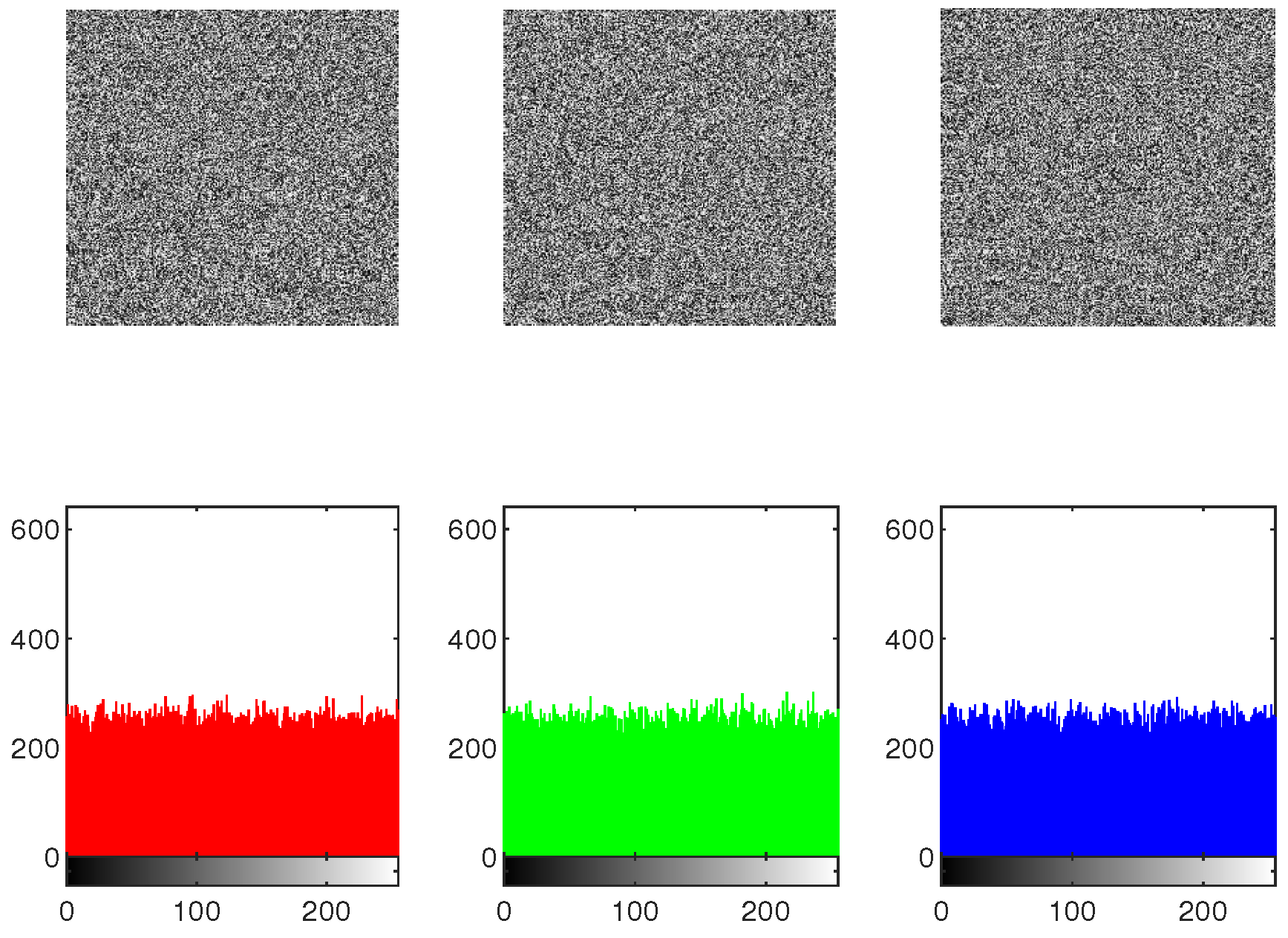
5.7.1. Histograms Analysis
The effectiveness of the IEA is obtained by comparing the histograms of the original as well as encrypted images. To protect against statistical attacks, it is crucial that there is no statistical similarity among the plaintext image and the encrypted image. The histogram analysis for the original image, shuffled image, encrypted image, and decrypted image of Mandrill across the , and channels is presented in Figure 20, Figure 21 and Figure 22. As illustrated in Figure 22, the histograms of the components of the encrypted image exhibit a flat distribution. Thus, in terms of histogram analysis, this algorithm is sufficiently robust to resist statistical attacks.
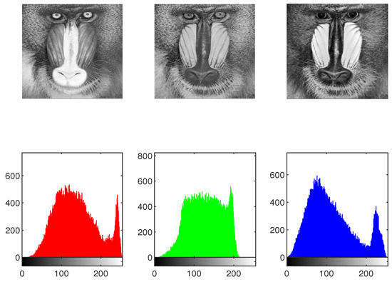
Figure 20.
The histogram of original image “Mandrill”.
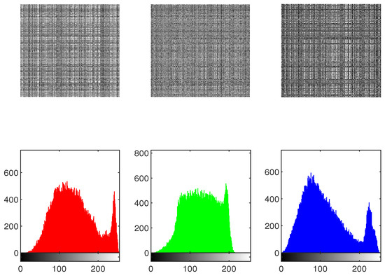
Figure 21.
The histogram of shuffled image “Mandrill”.
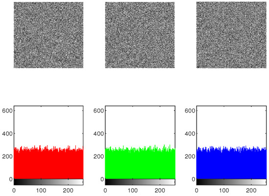
Figure 22.
The histogram of encrypted image “Mandrill”.
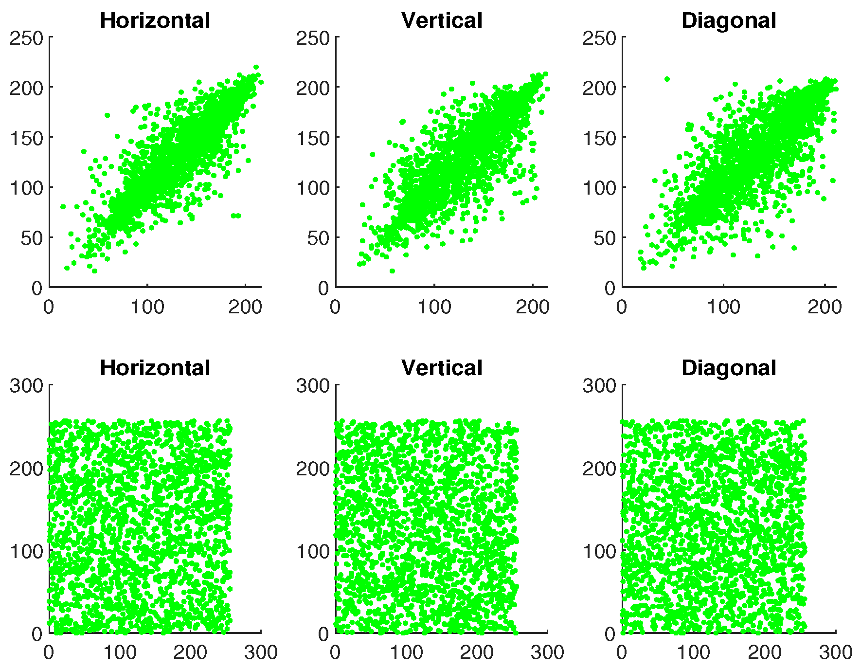
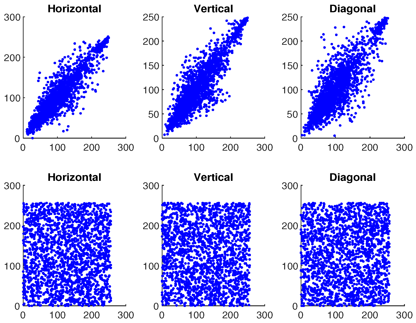
5.7.2. Correlation Coefficient Analysis
To analyze the performance of an IE algorithm, correlation analysis is also an important metric. It helps determine the level of similarity between adjacent pixels in an image. The CC is measured over the range of , where the or indicates that two pictures are identically same, and indicates that two pictures are completely unrelated. The CC is determined as follows:
where and ; O represents the total number pixels; and ♭, ♮ are the color values of the two adjacent pixels in the images. Table 1 shows the correlation values for plaintext and ciphertext of the image ‘Mandrill’. In addition, Figure 23, Figure 24 and Figure 25 illustrate the pixel distribution of plaintext image and ciphertext image of Mandrill on three color channels in horizontal (H), vertical (V), and diagonal (D) directions. Figure 23, Figure 24 and Figure 25 and Table 1 demonstrate the effectiveness of our algorithm and the security of the IE.

Table 1.
The CCs of Mandrill, Lion, and Peppers.
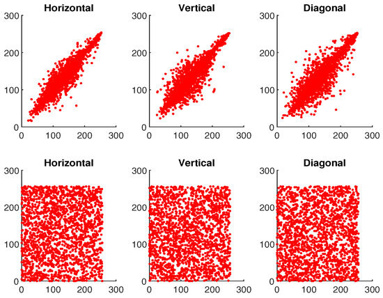
Figure 23.
The first and second rows demonstrate the correlation analysis for original and encrypted image of “Mandrill” in red channel.
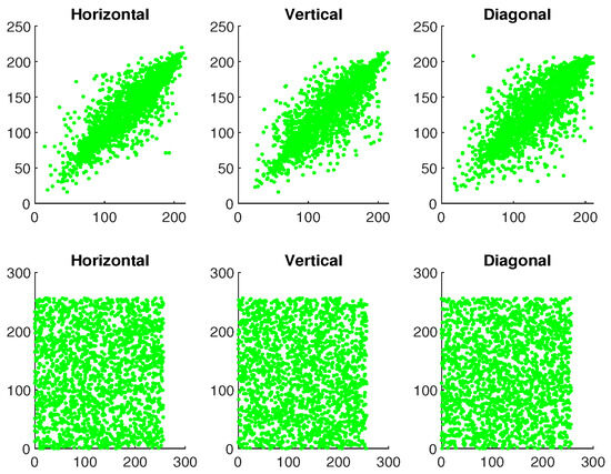
Figure 24.
The first and second rows demonstrate the correlation analysis for original and encrypted image of “Mandrill” in green channel.
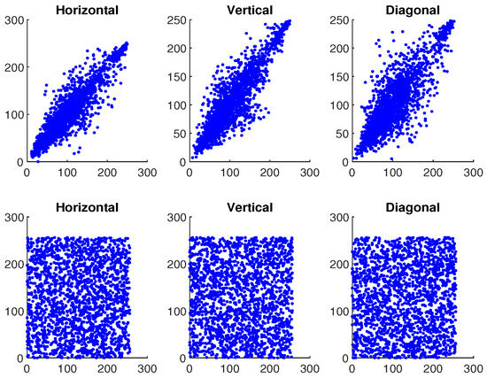
Figure 25.
The first and second rows demonstrate the correlation analysis for original and encrypted image of “Mandrill” in blue channel.
5.7.3. Information Entropy Analysis
The IE helps to quantify the level of uncertainty associated with an image. When it comes to IEA, the IE of the ciphered image needs to be as close to 8 as possible. This indicates that an encrypted image with a greater entropy measure signifies a stronger level of security. Thus, IE serves as an essential measurement for evaluating the performance of an encryption scheme. Generally, the entropy can be obtained by
in which represents the probability associated with grayscale value . Then, the IE results for the ciphered images derived from the plaintext images are presented in Table 2. Based on Table 2, the entropy value for the encrypted images is nearly 8, demonstrating its effectiveness. As a result of the high entropy value, the encrypted images are more secure against attacks because they have a higher level of randomness. Furthermore, we compared the IE generated by our algorithm with other existing quaternion-based encryption algorithms, as shown in Table 3. From Table 3, it can be observed that the image produced by our algorithm has the highest IE, demonstrating that our IEA offers significant performance.
Table 2.
The IE of Mandrill, Lion and Peppers.
Table 3.
The comparison of IE values of Mandrill cipher image.
5.8. Differential Attack Analysis
Recently, many IEAs have been cracked by attackers using differential attacks. Therefore, an efficient IEA must be highly sensitive to slight changes in the plain image. For an IEA, even a minor modification in the plain image should result in a significantly different encrypted image. The NPCR and UACI are metrics used to assess the resistance of an IEA to differential attacks. Also, NPCR and UACI can be obtained mathematically as follows:
in which and denote the images whose differences have to be determined, where the size of both images is ; denotes the difference among the images and based on the pixel . When , ; otherwise, .
The results are presented in Table 4. The optimal level of NPCR and UACI are and . Table 4 demonstrates that changing a pixel value in each channel yields NPCR and UACI values near the optimal level. So, it is evident that the proposed IEA is highly sensitive to minor changes in the image, even when only a single bit is altered. This demonstrates that the proposed IEA is more effective in resisting differential attacks.
Table 4.
The NPCR and UACI scores for different images.
5.9. Efficient Analysis
Additionally to security, improving IEA efficiency is another key motivation for researchers to design a new IEA. As a result, a well-designed IEA should not only be extremely secure, but also very efficient with respect to encryption. This section focuses on evaluating the efficiency of the proposed IEA by testing it on three distinct images of varying sizes. Here, we choose a Mandrill image of size, Lion image of size and Peppers image of size to verify the efficiency. Images with a larger size have a higher level of complexity. The encryption times based on this IEA are given in Table 5. From Table 5, we can observe that the proposed IEA is efficient in terms of encryption time.
Table 5.
The encryption time (in seconds) for different images using IEA.
6. Conclusions
This paper explored the GES problem for a class of QVNNs with discrete time-varying delays by using MMM. The results of this paper are derived through two methods. The first method is to address the non-commutative property of quaternion multiplication by decomposing the original QVNNs into equivalent four RVNNs. Then, by employing Lyapunov functions, Halanay’s inequality, and MMM, we established new solid criteria to ensure the GES of QVNNs under designed control. The second method examines the non-commutative property of quaternion multiplication directly; the original QVNNs are examined using the non-decomposition method, and corresponding GES criteria are derived. Furthermore, this paper presents novel results and new insights into GES of QVNNs. Finally, two numerical verifications with simulation results are given to verify the feasibility of the obtained criteria. Based on the considered master–slave QVNNs, a new IEA for color images Mandrill , Lion , and Peppers is proposed. In addition, the effectiveness of the proposed IEA is verified by various experimental analysis. The experiment results show that the algorithm has good CCs, IE with an average of 7.9988, NPCR with an average of 99.6080%, and UACI with an average of 33.4589%, and the results indicate that the IEA is robust against a range of security attacks. In addition, the results presented in this paper may be applied to more detailed investigations of various QVNN-related problems. Therefore, our future research will be focused on impulsive synchronization of QVNNs via an event-triggered impulsive controller and its application to secure communication.
Author Contributions
Conceptualization, R.S. and O.K.; methodology, R.S. and O.K.; software, R.S.; validation, O.K.; formal analysis, R.S. and O.K.; investigation, R.S. and O.K.; resources, R.S.; data curation, R.S.; writing—original draft preparation, R.S. and O.K.; writing—review and editing, R.S. and O.K.; visualization, R.S.; supervision, O.K.; project administration, R.S. and O.K.; funding acquisition, R.S. and O.K. All authors have read and agreed to the published version of the manuscript.
Funding
This work was fully supported by the Empowerment and Equity Opportunities for Excellence in Science program funded by the Science and Engineering Research Board (SERB), Government of India under grant EEQ/2023/000513. In addition, the work of second author was supported by the Basic Science Research Program through the National Research Foundation of Korea (NRF) funded by the Ministry of Education under Grant NRF-2020R1A6A1A12047945 and in part by Innovative Human Resource Development for Local Intellectualization program through the Institute of Information & Communications Technology Planning & Evaluation (IITP) grant funded by the Korea government (MSIT) (IITP-2024-2020-0-01462, 30%).
Data Availability Statement
The original contributions presented in the study are included in the article, further inquiries can be directed to the corresponding author.
Acknowledgments
The first author is grateful to the Science and Engineering Research Board (SERB), Government of India, for financial support. The second author further expresses gratitude to the National Research Foundation (NRF) for funding provided by the Basic Science Research Program. The authors also express their gratitude to the handling editor and reviewers for their valuable comments and suggestions regarding this manuscript.
Conflicts of Interest
The authors declare no conflicts of interest.
References
- Jayawardana, R.; Bandaranayake, T.S. Analysis of optimizing neural networks and artificial intelligent models for guidance, control, and navigation systems. Int. Res. J. Mod. Eng. Technol. Sci. 2021, 3, 743–759. [Google Scholar]
- Yu, Z.; Abdulghani, A.M.; Zahid, A.; Heidari, H.; Imran, M.A.; Abbasi, Q.H. An overview of neuromorphic computing for artificial intelligence enabled hardware-based hopfield neural network. IEEE Access 2020, 8, 67085–67099. [Google Scholar] [CrossRef]
- Liao, T.L.; Wang, F.C. Global stability for cellular neural networks with time delay. IEEE Trans. Neural Netw. 2000, 11, 1481–1484. [Google Scholar] [PubMed]
- Zhang, Z.; Quan, Z. Global exponential stability via inequality technique for inertial BAM neural networks with time delays. Neurocomputing 2015, 151, 1316–1326. [Google Scholar] [CrossRef]
- Huang, H.; Cao, J.; Wang, J. Global exponential stability and periodic solutions of recurrent neural networks with delays. Phys. Lett. A 2002, 298, 393–404. [Google Scholar] [CrossRef]
- Cai, Z.; Huang, L. Existence and global asymptotic stability of periodic solution for discrete and distributed time-varying delayed neural networks with discontinuous activations. Neurocomputing 2011, 74, 3170–3179. [Google Scholar] [CrossRef]
- Guo, R.; Zhang, Z.; Liu, X.; Lin, C. Existence, uniqueness, and exponential stability analysis for complex-valued memristor-based BAM neural networks with time delays. Appl. Math. Comput. 2017, 311, 100–117. [Google Scholar] [CrossRef]
- Yuan, Y.; Song, Q.; Liu, Y.; Alsaadi, F.E. Synchronization of complex-valued neural networks with mixed two additive time-varying delays. Neurocomputing 2019, 332, 149–158. [Google Scholar] [CrossRef]
- Zhou, B.; Song, Q. Stability and Hopf bifurcation analysis of a tri-neuron BAM neural network with distributed delay. Neurocomputing 2012, 82, 69–83. [Google Scholar] [CrossRef]
- Hirose, A. Nature of complex number and complex-valued neural networks. Front. Inf. Technol. Electron. Eng. 2011, 6, 171–180. [Google Scholar] [CrossRef]
- Nitta, T. Orthogonality of decision boundaries in complex-valued neural networks. Neural Comput. 2004, 16, 73–97. [Google Scholar] [CrossRef] [PubMed]
- Lee, D.L. Relaxation of the stability condition of the complex-valued neural networks. IEEE Trans. Neural Netw. 2001, 12, 1260–1262. [Google Scholar] [PubMed]
- Zhang, F. Quaternions and matrices of quaternions. Linear Algebra Appl. 1997, 251, 21–57. [Google Scholar] [CrossRef]
- Liu, Y.; Zheng, Y.; Lu, J.; Cao, J.; Rutkowski, L. Constrained quaternion-variable convex optimization: A quaternion-valued recurrent neural network approach. IEEE Trans. Neural Netw. Learn. Syst. 2019, 31, 1022–1035. [Google Scholar] [CrossRef]
- Liu, L.; Lei, M.; Bao, H. Event-triggered quantized quasisynchronization of uncertain quaternion-valued chaotic neural networks with time-varying delay for image encryption. IEEE Trans. Cybern. 2022, 53, 3325–3336. [Google Scholar] [CrossRef]
- Song, Q.; Long, L.; Zhao, Z.; Liu, Y.; Alsaadi, F.E. Stability criteria of quaternion-valued neutral-type delayed neural networks. Neurocomputing 2020, 412, 287–294. [Google Scholar] [CrossRef]
- Xu, X.; Xu, Q.; Yang, J.; Xue, H.; Xu, Y. Further research on exponential stability for quaternion-valued neural networks with mixed delays. Neurocomputing 2020, 400, 186–205. [Google Scholar] [CrossRef]
- Duan, H.; Peng, T.; Tu, Z.; Qiu, J.; Lu, J. Globally exponential stability and globally power stability of quaternion-valued neural networks with discrete and distributed delays. IEEE Access 2020, 8, 46837–46850. [Google Scholar] [CrossRef]
- Meng, X.; Li, Y. Pseudo almost periodic solutions for quaternion-valued cellular neural networks with discrete and distributed delays. J. Inequal. Appl. 2018, 2018, 245. [Google Scholar] [CrossRef]
- Lin, D.; Zhang, Q.; Chen, X.; Li, Z.; Wang, S. A color image encryption using one quaternion-valued neural network. SSRN Electron J. 2022, 4, 1–29. [Google Scholar] [CrossRef]
- Tu, Z.; Zhao, Y.; Ding, N.; Feng, Y.; Zhang, W. Stability analysis of quaternion-valued neural networks with both discrete and distributed delays. Appl. Math. Comput. 2019, 343, 342–353. [Google Scholar] [CrossRef]
- Pecora, L.M.; Carroll, T.L. Synchronization in chaotic systems. Phys. Rev. Lett. 1990, 64, 821. [Google Scholar] [CrossRef]
- Alsaedi, A.; Cao, J.; Ahmad, B.; Alshehri, A.; Tan, X. Synchronization of master-slave memristive neural networks via fuzzy output-based adaptive strategy. Chaos Solitons Fractals 2022, 158, 112095. [Google Scholar] [CrossRef]
- Xu, D.; Wang, T.; Liu, M. Finite-time synchronization of fuzzy cellular neural networks with stochastic perturbations and mixed delays. Circuits Syst. Signal Process. 2021, 40, 3244–3265. [Google Scholar] [CrossRef]
- Peng, T.; Zhong, J.; Tu, Z.; Lu, J.; Lou, J. Finite-time synchronization of quaternion-valued neural networks with delays: A switching control method without decomposition. Neural Netw. 2022, 148, 37–47. [Google Scholar] [CrossRef] [PubMed]
- Samidurai, R.; Sriraman, R. Non-fragile sampled-data stabilization analysis for linear systems with probabilistic time-varying delays. J. Frank. Inst. 2019, 356, 4335–4357. [Google Scholar] [CrossRef]
- Samidurai, R.; Sriraman, R.; Zhu, S. Stability and dissipativity analysis for uncertain Markovian jump systems with random delays via new approach. Int. J. Syst. Sci. 2019, 50, 1609–1625. [Google Scholar] [CrossRef]
- Sriraman, R.; Cao, Y.; Samidurai, R. Global asymptotic stability of stochastic complex-valued neural networks with probabilistic time-varying delays. Math. Comput. Simul. 2020, 171, 103–118. [Google Scholar] [CrossRef]
- He, W.; Cao, J. Exponential synchronization of chaotic neural networks: A matrix measure approach. Nonlinear Dyn. 2009, 55, 55–65. [Google Scholar] [CrossRef]
- Li, Y.; Li, C. Matrix measure strategies for stabilization and synchronization of delayed BAM neural networks. Nonlinear Dyn. 2016, 84, 1759–1770. [Google Scholar] [CrossRef]
- Gong, W.; Liang, J.; Cao, J. Matrix measure method for global exponential stability of complex-valued recurrent neural networks with time-varying delays. Neural Netw. 2015, 70, 81–89. [Google Scholar] [CrossRef]
- Tang, Q.; Jian, J. Matrix measure based exponential stabilization for complex-valued inertial neural networks with time-varying delays using impulsive control. Neurocomputing 2018, 273, 251–259. [Google Scholar] [CrossRef]
- Xie, D.; Jiang, Y.; Han, M. Global exponential synchronization of complex-valued neural networks with time delays via matrix measure method. Neural Process. Lett. 2019, 49, 187–201. [Google Scholar] [CrossRef]
- Kocak, O.; Erkan, U.; Toktas, A.; Gao, S. PSO-based image encryption scheme using modular integrated logistic exponential map. Expert Syst. Appl. 2024, 237, 121452. [Google Scholar] [CrossRef]
- Toktas, F.; Erkan, U.; Yetgin, Z. Cross-channel color image encryption through 2D hyperchaotic hybrid map of optimization test functions. Expert Syst. Appl. 2024, 249, 123583. [Google Scholar] [CrossRef]
- Feng, W.; Wang, Q.; Liu, H.; Ren, Y.; Zhang, J.; Zhang, S.; Wen, H. Exploiting newly designed fractional-order 3D Lorenz chaotic system and 2D discrete polynomial hyper-chaotic map for high-performance multi-image encryption. Fractal Fract. 2023, 7, 887. [Google Scholar] [CrossRef]
- Feng, W.; Zhao, X.; Zhang, J.; Qin, Z.; Zhang, J.; He, Y. Image encryption algorithm based on plane-level image filtering and discrete logarithmic transform. Mathematics 2022, 10, 2751. [Google Scholar] [CrossRef]
- Wen, H.; Lin, Y. Cryptanalysis of an image encryption algorithm using quantum chaotic map and DNA coding. Expert Syst. Appl. 2024, 237, 121514. [Google Scholar] [CrossRef]
- Wen, H.; Lin, Y. Cryptanalyzing an image cipher using multiple chaos and DNA operations. J. King Saud Univ.-Comput. Inf. Sci. 2023, 35, 101612. [Google Scholar] [CrossRef]
- Feng, W.; Zhang, J. Cryptanalzing a novel hyper-chaotic image encryption scheme based on pixel-level filtering and DNA-level diffusion. IEEE Access 2020, 8, 209471–209482. [Google Scholar] [CrossRef]
- Vidyasagar, M. Nonlinear Systems Analysis; Prentice-Hall: Englewood Cliffs, NJ, USA, 1993. [Google Scholar]
- Chen, M. Chaos synchronization in complex networks. IEEE Trans. Circuits Syst. I Regul. Pap. 2008, 55, 1335–1346. [Google Scholar] [CrossRef]
- Cheng, C.J.; Liao, T.L.; Hwang, C.C. Exponential synchronization of a class of chaotic neural networks. Chaos Solitons Fractals 2005, 24, 197–206. [Google Scholar] [CrossRef]
- Chen, X.; Song, Q.; Li, Z. Design and analysis of quaternion-valued neural networks for associative memories. IEEE Trans. Syst. Man Cybern. 2017, 48, 2305–2314. [Google Scholar] [CrossRef]
- Zhang, Y.; Yang, L.; Kou, K.I.; Liu, Y. Synchronization of fractional-order quaternion-valued neural networks with image encryption via event-triggered impulsive control. Knowl.-Based Syst. 2024, 296, 111953. [Google Scholar] [CrossRef]


Disclaimer/Publisher’s Note: The statements, opinions and data contained in all publications are solely those of the individual author(s) and contributor(s) and not of MDPI and/or the editor(s). MDPI and/or the editor(s) disclaim responsibility for any injury to people or property resulting from any ideas, methods, instructions or products referred to in the content. |
© 2024 by the authors. Licensee MDPI, Basel, Switzerland. This article is an open access article distributed under the terms and conditions of the Creative Commons Attribution (CC BY) license (https://creativecommons.org/licenses/by/4.0/).