Abstract
This article delivers a new Preisach model representing the correlation between the elastoplastic behavior of structural mild steel under axial monotonic and cyclic loading with damage. The newly formed model is based on the experimentally defined correlation between axial monotonic and cyclic behavior of structural mild steel. To examine the monotonic and cyclic behavior of structural mild steel and find fitting material properties for the model, monotonic and cyclic axial tensile tests are performed. Tests are executed on coupons of the commonly used European structural steel S275. The model represents a mathematical description of modified single-crystal material behavior under monotonic loading. Two different approaches were used to describe damage in the multilinear mechanical model. The excellent agreement with experimental results is achieved by infinitely linking many single-crystal elements in parallel, forming the polycrystalline model. This model provides a good solution for everyday engineering practice due to its geometric representation in the form of the Preisach triangle and the lower costs of monotonic tests used to define material properties compared to cyclic tests.
Keywords:
monotonic axial strain; cyclic loading; Preisach model; hysteresis loop; hysteresis skeleton curve MSC:
74C15
1. Introduction
Elasto-plastic behavior of structural mild steel members is very important in structural design. Under cyclic loading, the working stress level exceeds the elastic limit and becomes much higher than under monotonic loading [1]. A typical representative of cyclic loading is seismic loading, characterized by repeated inelastic strains. Earthquakes are natural disasters that can cause significant damage to buildings, infrastructure, and human life [2]. When an earthquake occurs, the mild steel structural members may experience small numbers of large displacement cycles, where the material is working well within the inelastic range. The performance of structural steel members to seismic loading is affected by their geometrical characteristics and by the hysteretic response of the structural steel material [3]. The cyclic response of structural steel material under large inelastic strains, counting the Bauschinger effect, cyclic softening or hardening, and damage accumulation, is much different from its monotonic response [4]. Structural mild steels have a characteristic yield plateau in their stress–strain monotonic response, which vanishes under cyclic loading.
An accurate description of material behavior is essential for precise and reliable response prediction of the member or structure under monotonic or cyclic loading.
While there is a significant amount of experimental data available on cyclic plasticity of structural steel, there are a limited number of published papers on cyclic deformation at large strain ranges due to limitations in test setups and issues with specimen buckling [5,6,7]. This paper presents an experimental investigation on the stress–strain characteristics of structural mild steel subjected to large repeated cyclic plastic deformations. The experimental program aimed to compare the material behavior under monotonic and cyclic loading and to establish a correlation between them. Additionally, the study examined the effects of loading history on the cyclic response of structural mild steel.
The cyclic behavior of mild structural steel has been studied experimentally by various authors [8,9]. Their results reveal that the material’s cyclic characteristics are not accurately portrayed by the monotonic hardening curve. However, for proportional loading, there is a specific cyclic loading amplitude for which the stabilized stress amplitude will align with the monotonic stress–strain curve [8]. When fully reversed cyclic amplitudes exceed this value, cyclic hardening occurs, while for amplitudes smaller than this value, the stabilized stress does not surpass the initial yield stress under monotonic loading. Regardless of the loading amplitude, the stress–strain loops are smooth without any irregularities and display a strong Bauschinger effect.
Currently, different constitutive models are widely used in the design of structural elements. However, defining a precise constitutive model for cyclic loading requires accurate knowledge of the material behavior and its properties. These values may be estimated by cyclic tests. Due to the high cost of cyclic tests in comparison to monotonic tests, the correlation of results must be achieved. In this paper, the correlation between these two types of behavior is established through the linkage of the hysteresis skeleton curve and monotonic loading curve.
2. Experimental Studies
2.1. Specimen Details
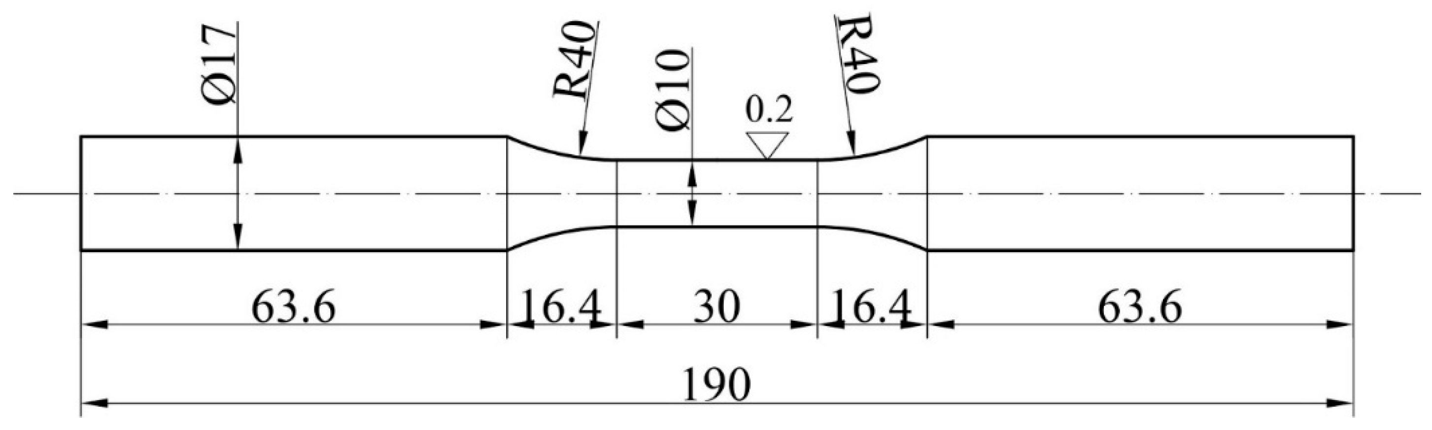
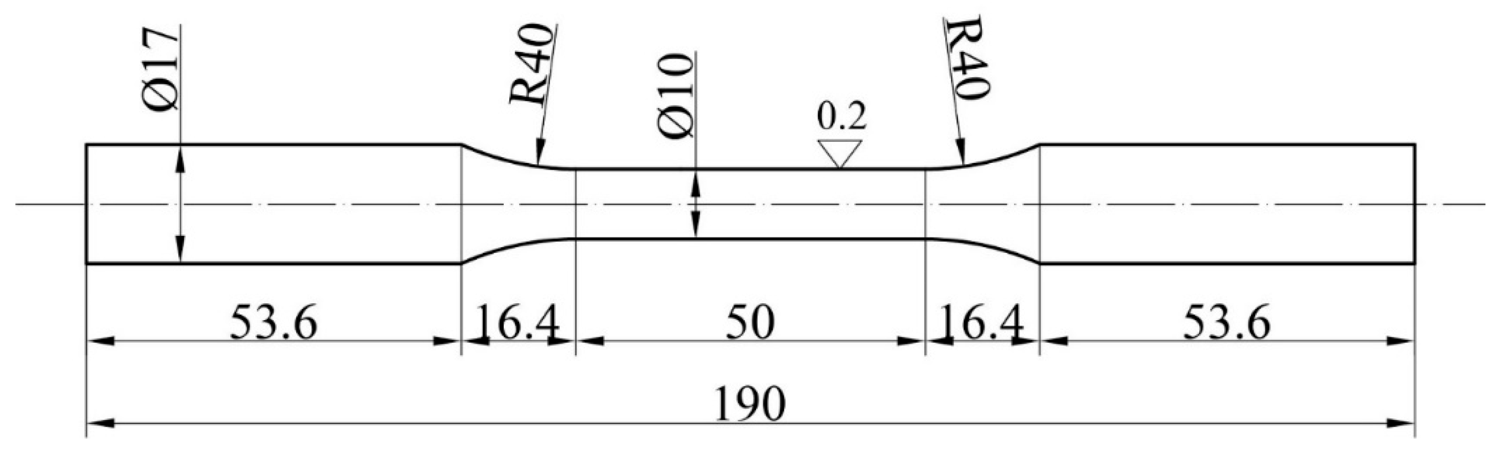
The structural steel type S275 is considered in this study. Observations are conducted on coupons produced from hot-rolled plates. The test specimens were cut in the rolling direction. The hot-rolled plates are thick enough to machine into round coupons. In order to prevent the coupons from buckling during compression, the test specimens were machined into round coupons with a reduced section effective length, following the test method for axial loading constant–amplitude low-cycle fatigue of metallic materials [10], as illustrated in Figure 1.
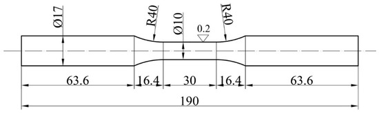
Figure 1.
Cyclic round coupon.
The coupons had a section diameter of 10 mm and a reduced length of 30 mm, resulting in a section length-to-diameter ratio of 3. The reduced area and transition zone were shaped using numerically controlled equipment to detour any undercut. To guarantee consistency across all tests, the surface finish was carefully polished using sandpaper. It is worth noting that standards for tensile test procedures, such as the American Society for Testing and Materials Standard [11] and Chinese Tensile Testing Standard [12], recommend large section length-to-diameter ratios for round coupons, as compression buckling is not considered. Because of those recommendations, coupons used for only tensile tests are as shown in Figure 2.

Figure 2.
Only tension round coupon.
To validate the results of the cyclic tension–compression tests, we compared the stress–strain curves acquired from a uniaxial tension test using the cyclic coupon sample (Figure 1) with those from a standard coupon specimen (Figure 2). The impact of the cyclic specimens’ head widening on the measured stress–strain responses is negligible.
2.2. Material Properties
Twenty monotonic tensile loading tests were conducted at room temperature in accordance with [13]. The tests were carried out at a constant strain rate of 3 mm/min. Standard coupon samples, as illustrated in Figure 2, were used in these monotonic tensile coupon tests to establish the fundamental engineering stress–strain characteristics of the material. The mean material properties obtained from the tensile coupon tests are summarized in Table 1. This includes the initial Young’s modulus E, upper yield point σuy, the lower yield point σly, Lüders strain εL, maximum stress σu, and strain εu under tension, and the stress and strain under fracture (σD, εD) established on a gauge length of 50 mm. The material properties we obtained were used to help analyze the results of the cyclic tests. It is important to note that we also conducted a monotonic tensile test on two cyclic coupon specimens, as illustrated in Figure 1, to validate the results of the cyclic tension–compression tests.

Table 1.
Mean values and standard deviation of material characteristics obtained from direct tensile tests.
2.3. Test Configuration and Loading Protocols
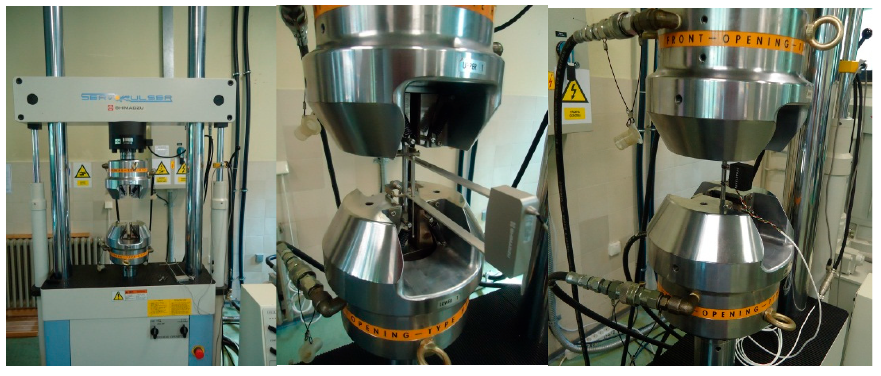
A total of six cyclic loading tests were conducted at room temperature following European Standard ISO 12106 [10]. The cyclic tension–compression loading tests were conducted on cyclic coupon specimens subjected to cyclic straining using a universal tension–compression fatigue loading machine SHIMADZU Servo Pulser at a strain rate of 0.1 Hz. This test’s rate minimizes the influence of temperature. Hydraulic grips were employed to secure the coupons, allowing for both tensile and compressive loads, as depicted in Figure 3.
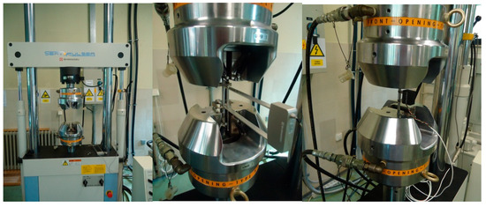
Figure 3.
Test equipment configuration.
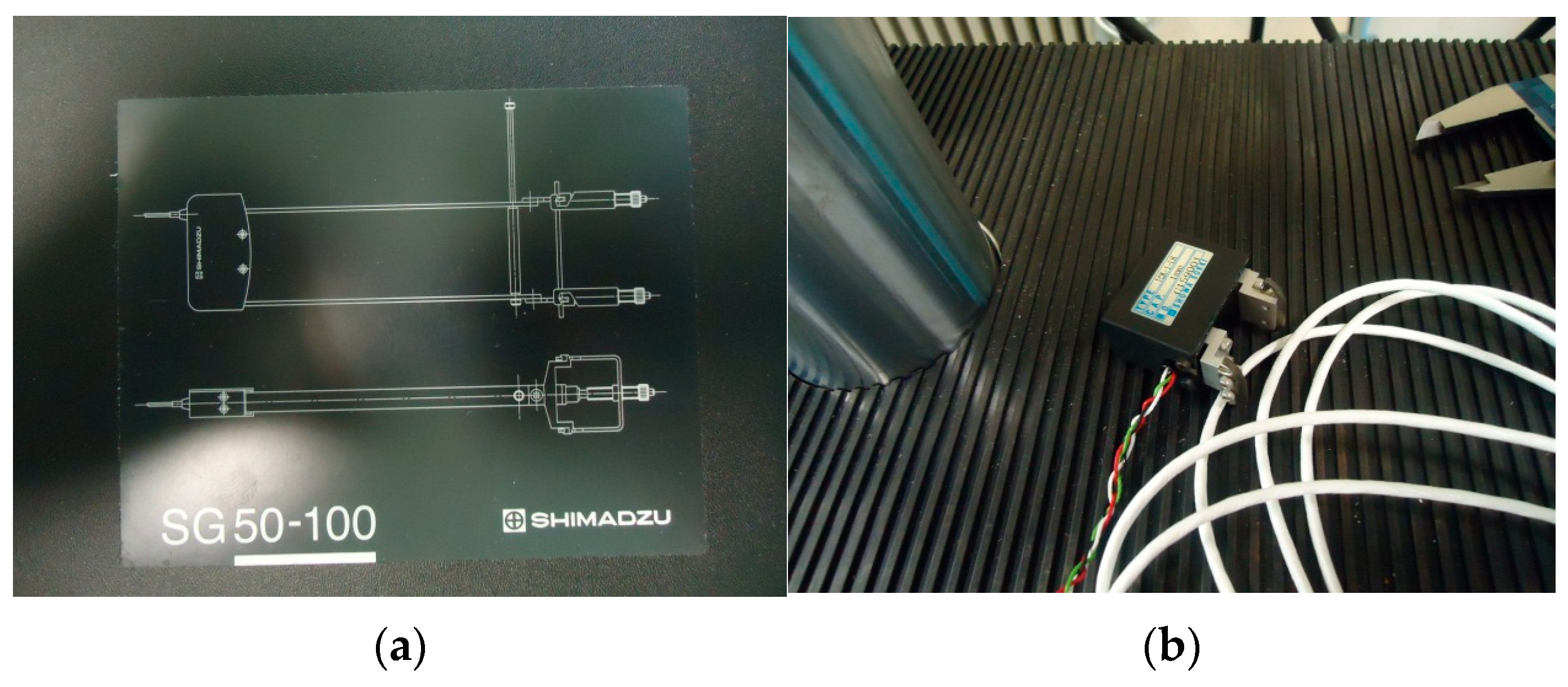
All of the tests were displacement controlled using the extensometer to eliminate the effect of possible grip slippage or deformation outside of the effective length. The extensometer SHIMADZU SG 50-100, Shimadzu, Kyoto, Japan (Figure 4a) with a gauge length of 50 mm was used for monotonic tests, while a SHOWA-SOKI TCK-1-IF extensometer Showa Sokki, Tokyo, Japan (Figure 4b) with a gauge length of 25 mm is used for cyclic tests.

Figure 4.
Extensometers used for (a) monotonic tests; (b) cyclic tests.
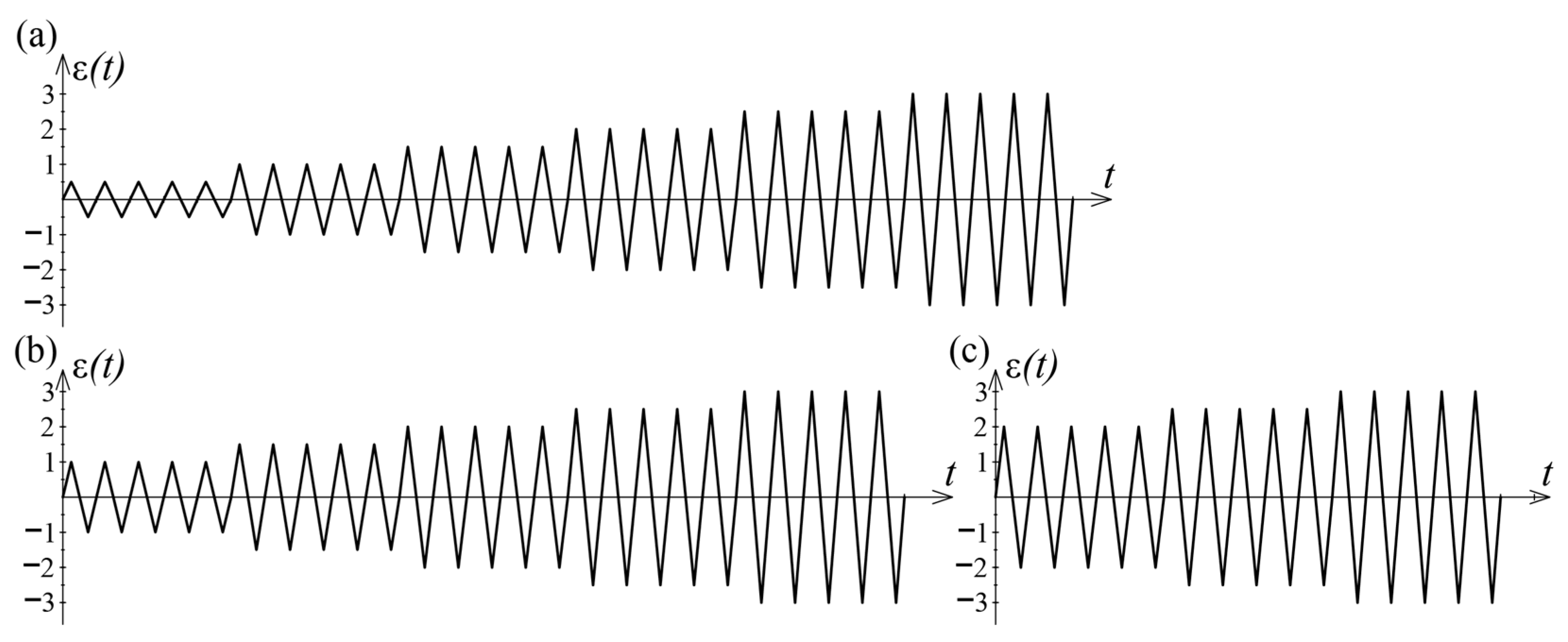
The cyclic ascend protocol was considered in this study, through three different load histories (A, B, and C), as shown in Figure 5. Load histories are formed with an equal strain increment of ±0.5% after each five-cycle loading phase up to ±3.0% but with different starting cycle amplitudes. Each strain amplitude was repeated for five cycles to obtain a fairly saturated response from the examined steel. The cyclic tests on two different coupons are conducted for each of the three load histories. The load histories, including the number of cycles for all samples tested under cyclic loading, are presented in Table 2. It is important to note that after completing a series of cyclic loading, each sample is first unloaded and then pulled until complete rupture under tension.

Figure 5.
Load histories for cyclic ascend load regime according to Table 2: (a) Load history A for coupons III-3 and III-4; (b) Load history B for coupons III-5 and III-6; (c) Load history A for coupons III-7 and III-8.
Table 2.
Number of cycles for different load histories.
The load, displacement, strain, and input stress were all measured using data acquisition equipment and logged using the SHIMADZU computer packages, TRAPEZIUMX-V.
2.4. Test Results
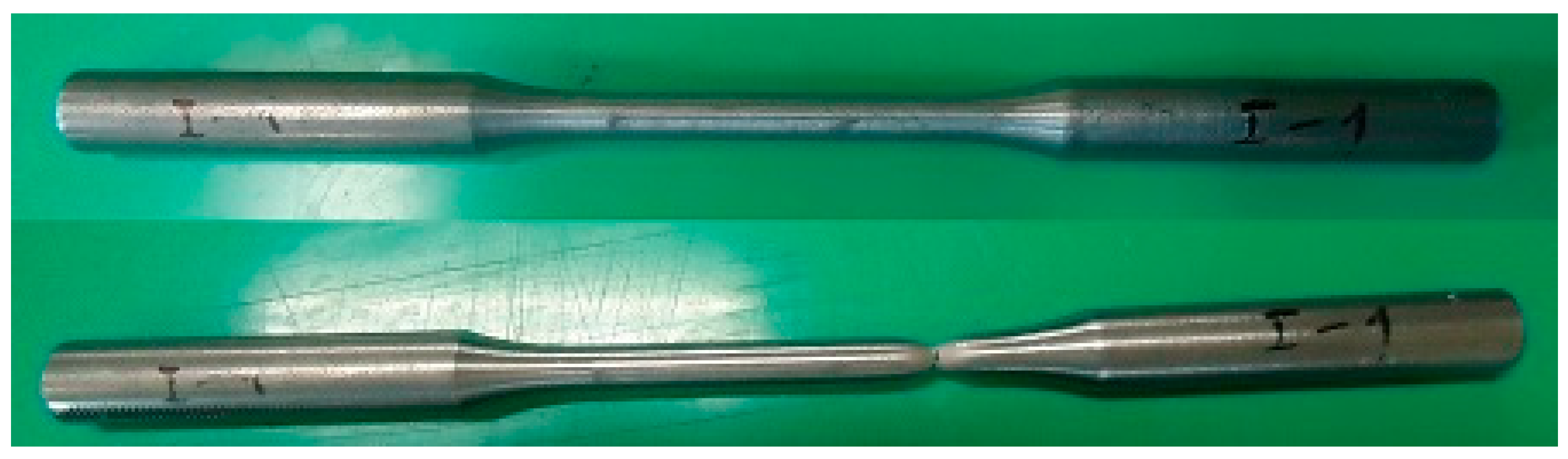
The failure modes observed in the monotonic tensile loading test samples and the cyclic tension–compression loading test samples on structural mild steel are shown in Figure 6 and Figure 7, respectively. Necking occurred for all the specimens. It is important to note that none of the test specimens exhibited buckling in compression.

Figure 6.
Failure modes for monotonic tension test specimens.
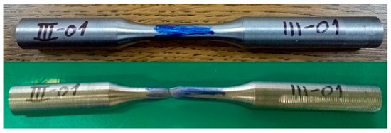
Figure 7.
Failure modes for cyclic tension–compression test specimens.
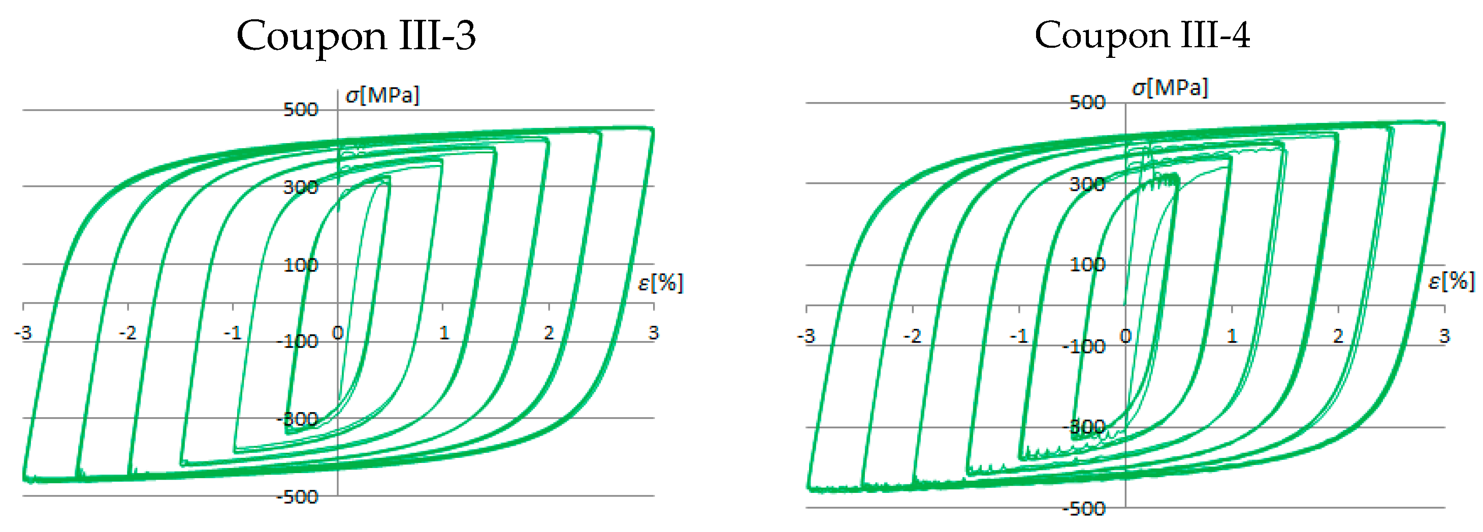
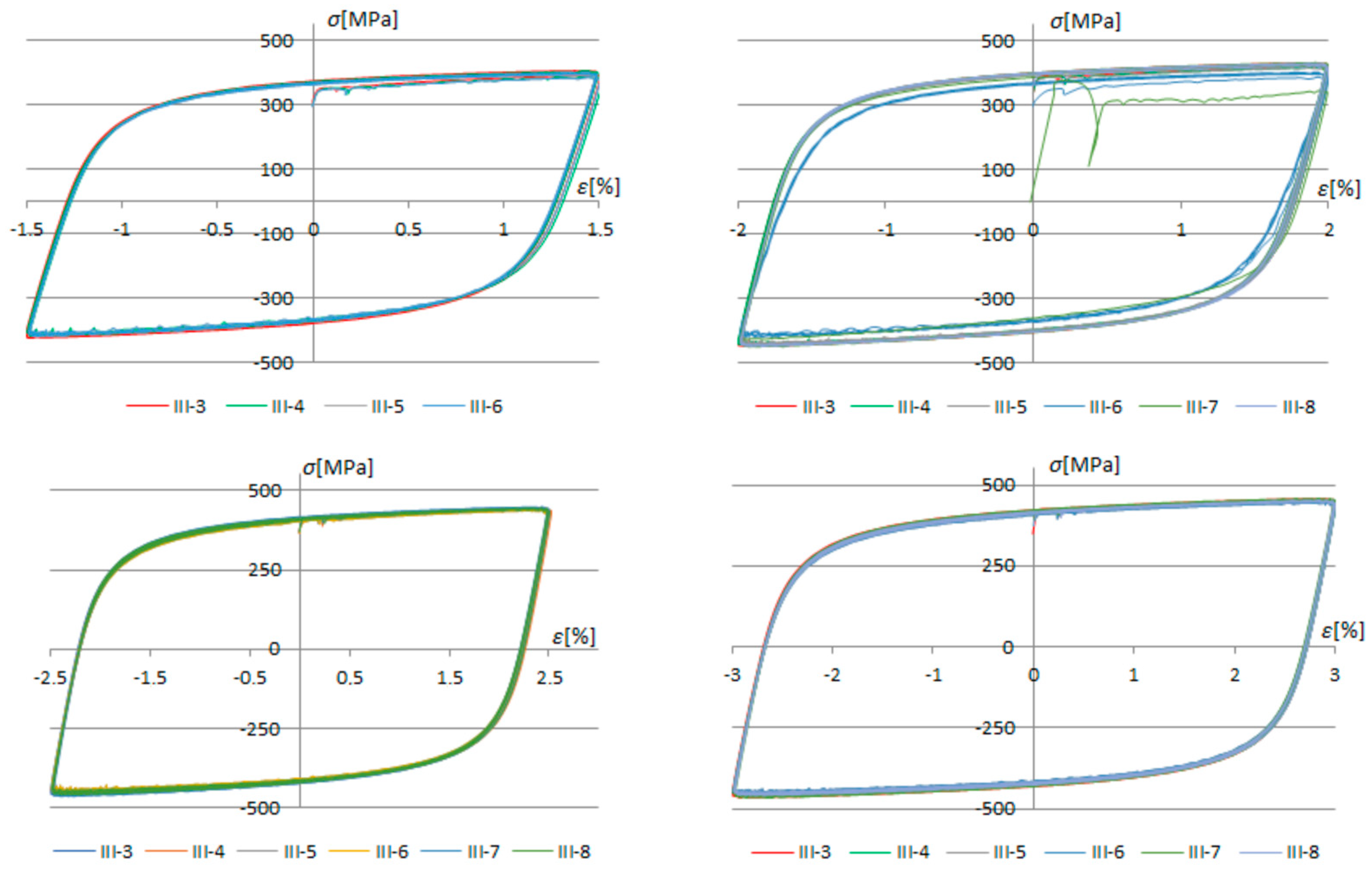
Stress–strain responses during cyclic loading are depicted in Figure 8, Figure 9 and Figure 10 for applied load histories. In the following figures, the coupon and load history can be identified via Table 2. The first index in the specimen label stands for the type of the test (I—monotonic tensile loading test; III—cyclic loading test), while the second index denotes an order number of coupons in the test method.
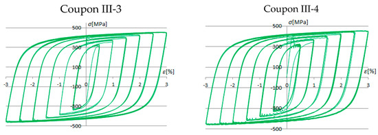
Figure 8.
Test results for cyclic load history A.
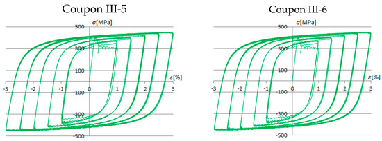
Figure 9.
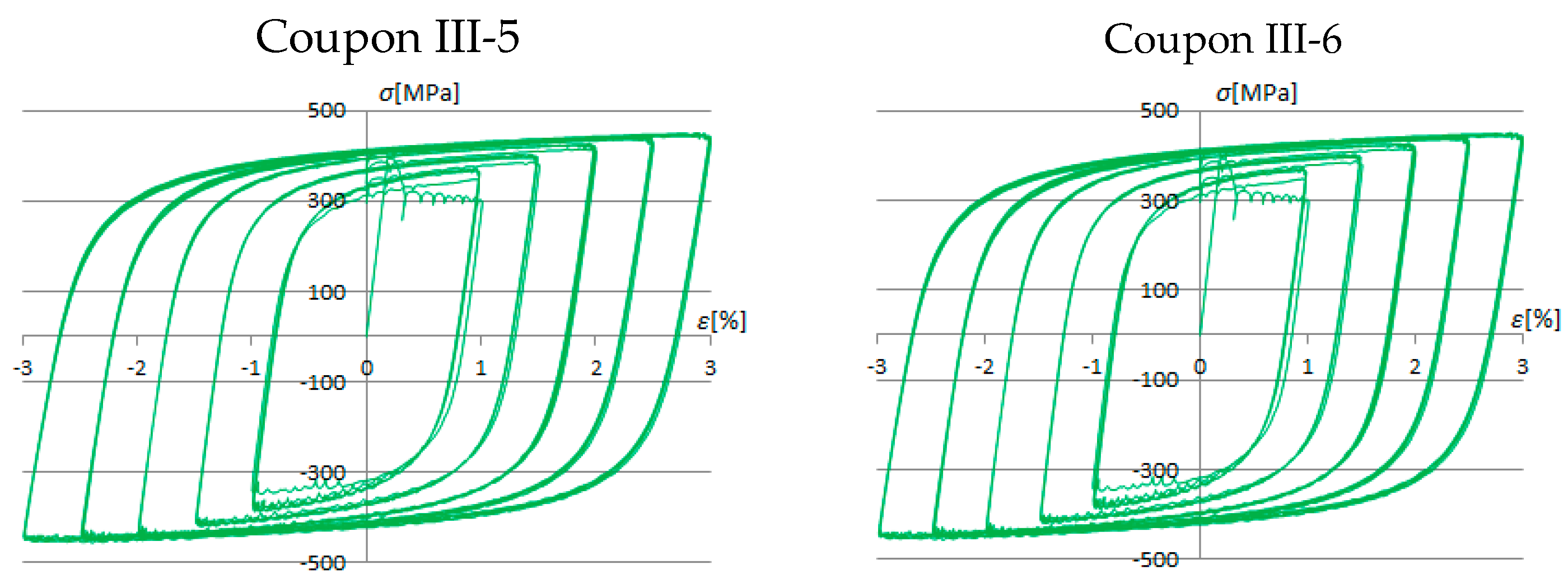
Test results for cyclic load history B.
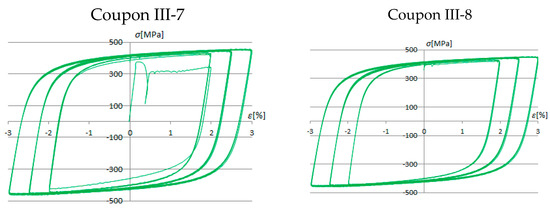
Figure 10.
Test results for cyclic load history C.
The experimental tests showed the formation of full, regular, and concentrated hysteresis loops, symmetrical to the origin.
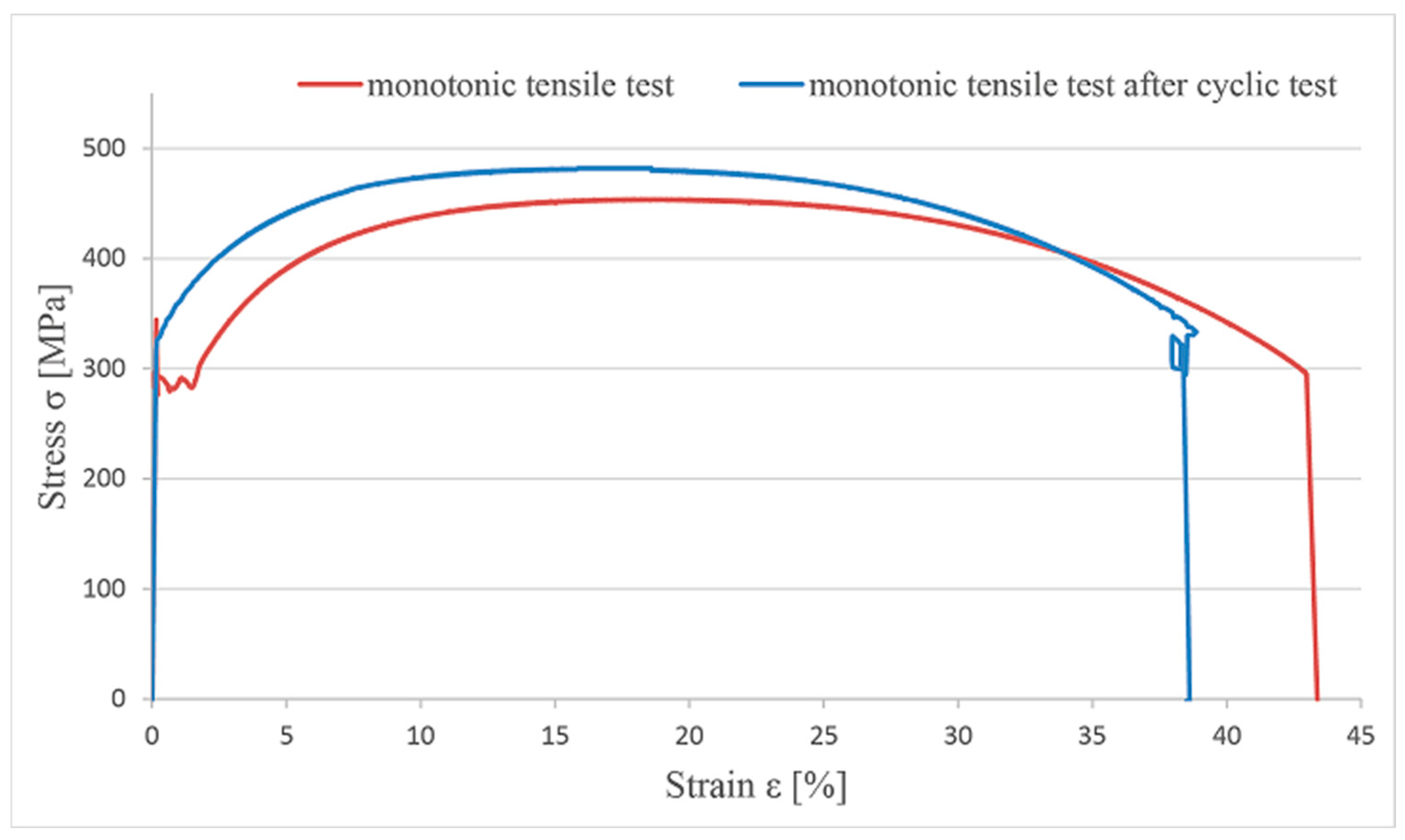
After subjecting the specimens to repeated cycles of loading, they are first unloaded and then stretched until complete fracture in tension occurs. The stress–strain curve of the monotonic tensile test on the cyclic coupon is compared with the curve of the final pull-out stage, depicted in Figure 11.
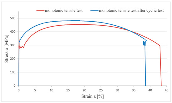
Figure 11.
The stress–strain curves obtained by monotonic tensile test, with and without previous cyclic load regimes.
3. Results and Discussion
The previous study shows a divergence in the material behavior under cyclic and monotonic loading. Local instability, materialized in the form of a yield plateau, disappears with the first change in loading direction. The Lüders band phenomenon does not occur under cyclic loading, so the Lüders strain is zero (εL = 0). This phenomenon occurs even under strain amplitudes that do not exceed the strain value of a horizontal plateau. Monotonic tensile tests after a cyclic test have shown a decreased ductility of steel under cyclic loading.
The stress values under cyclic testing are slightly higher than values under monotonic loading for the same values of strain. This phenomenon is a result of the cyclic hardening of the material. The effect of cyclic hardening is a change in the shape of the hysteresis loops, too. As a result, non-Massing material behavior occurs.
The experimental results of cyclic tests under the same load histories have shown excellent concurrence (Figure 10).
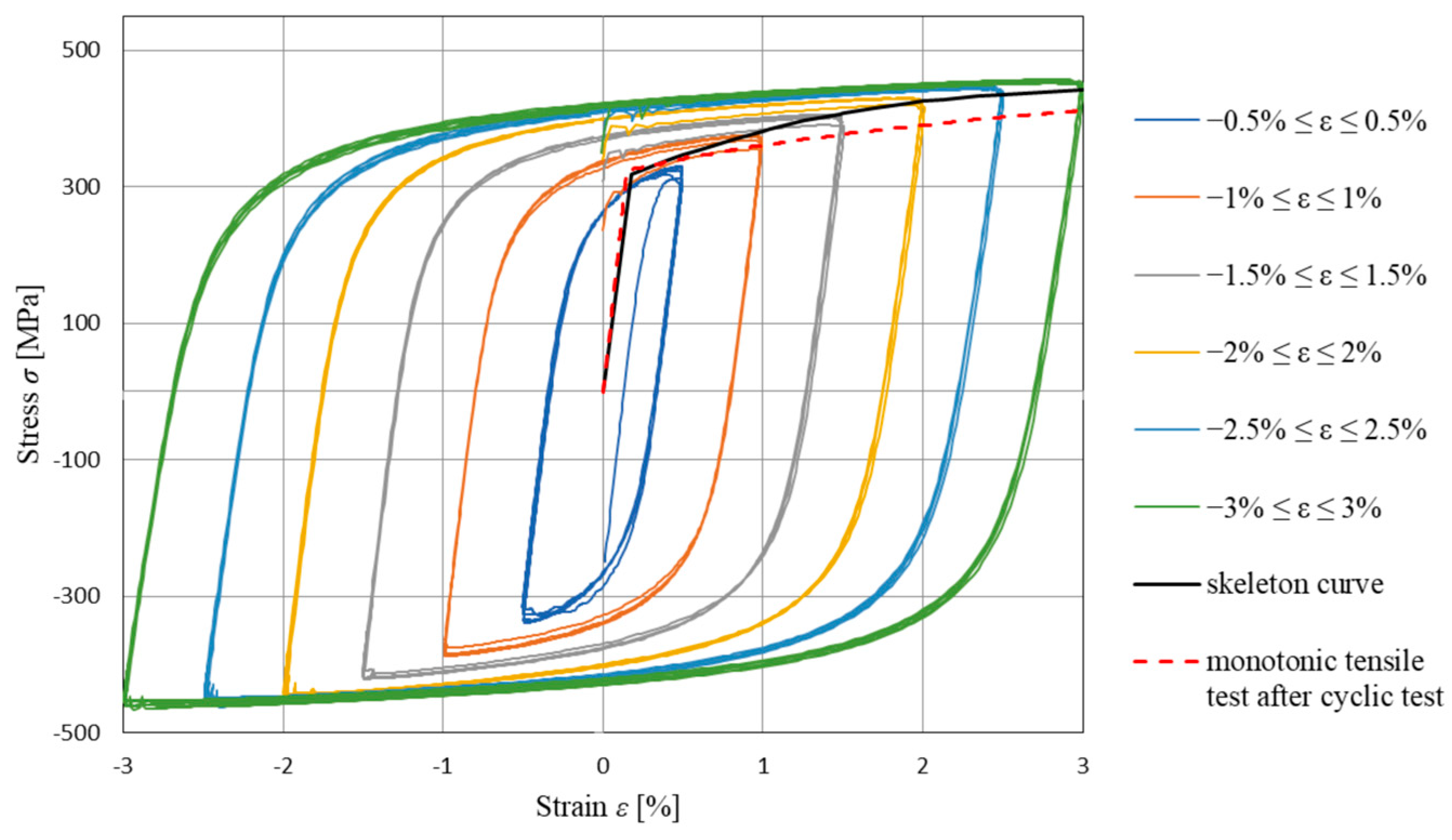
Since load histories were formed from blocks of cycles with constant amplitudes, arranged so that each subsequent block has a higher stress amplitude, each local extremum of the load history (Figure 5) will represent the maximum strain at the observed time, max ε(t). The comparability of hysteresis loops of the exact amplitudes formed under different loading histories is depicted in Figure 12.

Figure 12.
Comparison of hysteresis loops with the same amplitudes of the different samples.
The experiments have shown phenomenal concurrence of hysteresis loops with the same strain amplitudes ±ε(t), regardless of the applied load history (A, B, or C). This phenomenon is an outcome of the fact that the strain ε(t) under which hysteresis loops were formed represents the maximum strain in the observed load history up to the point in time t. That shows that the material characteristics defining hysteresis loop shape under cyclic loading depend only on the steel class and the maximum strain in the load history up to the observed moment in time t (previous load history). A line can be drawn through the peaks of hysteresis loops (Figure 13). This trend line is called the skeleton curve.
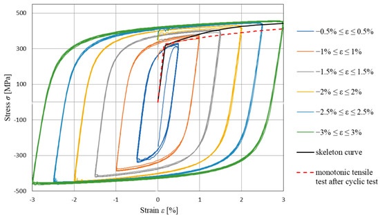
Figure 13.
Comparison of newly formed skeleton curve with monotonic and cyclic test results and its verification as a trend line for peaks of hysteresis loop.
The skeleton curve is formed based on experimental results. This trend line connecting peaks of hysteresis loops is characteristic of pure cyclic behavior. Meanwhile, it can be modeled through a modified stress–strain curve obtained from the monotonic tensile test. The modified monotonic stress–strain curve is formed by excluding the yield plateau and adopting twice faster stress increase in the material hardening zone for the same dilatation increase ε(t).
Structural mild steel behavior under cyclic loading is defined via material properties obtained from monotonic tensile tests.
4. Constitutive Model
The phenomenon of hysteresis occurs in many areas such as mechanics [14], ferromagnetism [15], seismology [16], engineering [17,18], economics [19], etc. Many phenomena in these areas are defined by the Preisach model, initially developed in 1935 to define hysteresis in ferromagnetism and is named after its author [20]. Its application in physics defines phenomena such as ferromagnetism, plasticity, and filtration through porous media. It has long been considered a physical operator, but M. Krasnoselski [21] separated this model from its physical form and presented it as a purely mathematical model.
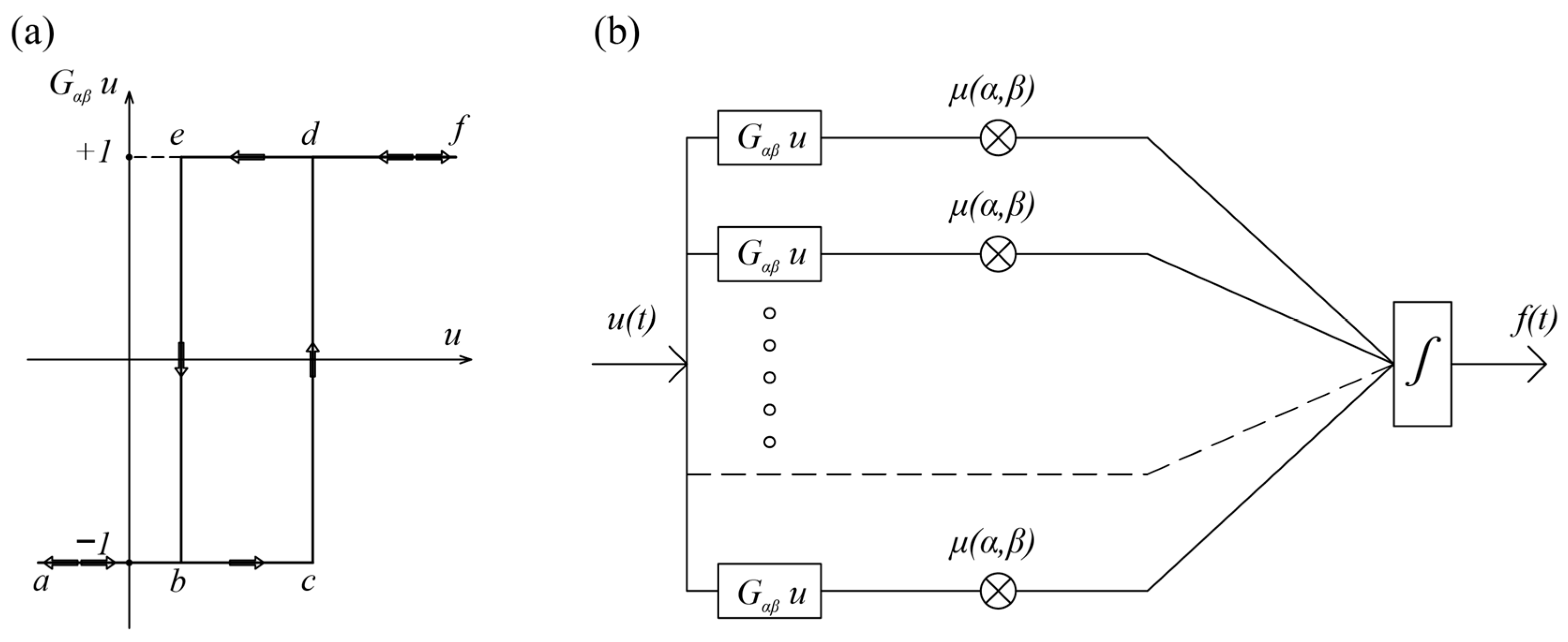
Preisach’s model maps the input data function into the output data function [22]. The basis of this model is the elementary nonlinear hysteresis operator Gα,β (Figure 14a), which is a discontinuous operator with local memory. Since the output can have only two values (+1 and −1), these operators are also called relay operators. However, by superposing these operators within the domain Γ (Figure 14b), the Preisach hysteresis operator is formed as a continuous system of infinitely many elementary operators connected in parallel (or in series):
where represents the Preisach weight function, according to which the elementary operators are arranged, and Gα,β is the elementary hysteresis operator.

Figure 14.
(a) Elementary hysteresis operator Gα,β; (b) Formation of the Preisach hysteresis model by superposition of elementary hysteresis operators.
Take into account the following:
- -
- After reaching the yield limit Y1, the monotone curve and skeleton curve are very different due to the effect of cyclic hardening;
- -
- The skeleton curve does not possess a yield plateau (εL = 0);
- -
- Although they differ, both monotonic and skeleton curves asymptotically strives for the same stress value σu [23].
Considering the above, it is possible to define the real behavior of mild steel under cyclic loading by upgrading the existing model for monotonic loading [24].
This article will present a new type of Preisach model designed to analyze the response of structural mild steel under constant cyclic ascending loading. Its basis is a model defining the behavior of this steel type under monotonic loading [24].
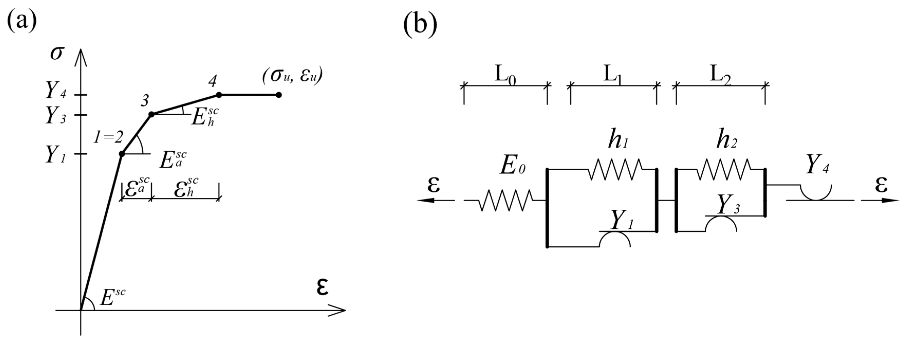
The main principle in modeling elastoplastic material behavior is based on defining an analog mechanical model, determined by an appropriate set of algebraic and/or differential equations. The mechanical model that describes the skeleton curve as the key indicator of behavior under cyclic loading, up to max stress σu, is shown in Figure 15a. The model is compiled of three Hook’s spring elements and three Saint-Venant’s slip elements.
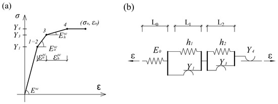
Figure 15.
(a) Quadruple linear working diagram and (b) mechanical model.
The concavity of the σ-ε skeleton curve in the hardening zone is achieved by its approximation with three lines, which makes the working diagram quadruple linear (Figure 15b).
The material properties of the mechanical model accomplished by connecting the spring elements in parallel or regular are defined below (2):
As the experiments showed, material properties defining the mechanical model from Figure 15b can be evaluated through mechanical properties obtained from monotonic tensile tests [24]. By excluding the horizontal plateau formed after reaching the yield strength Y1 (εL = 0) and adopting twice the strain increase in the hardening zone, the material properties of the skeleton curve can be defined as follows:
where stands for monotonic material properties and stands for skeleton curve material properties. The parameter ζ = 2 signifies the correlation coefficient between characteristics defining monotonic and cyclic behavior. It represents a doubling of the stress increase rate in the material hardening zone for the same increase in dilatation ε(t) during the formation of a modified monotonic stress–strain curve. This transformation converts the modified monotonic stress–strain curve into a compelling trend line composed of hysteresis loop peaks. With this procedure and the suggested value of ζ, the proposed skeleton curve model best fits the experimental data.
It is possible to define a new hysteresis mechanical model based on the working diagram shown in Figure 15a, which describes the cyclic skeleton curve of a structural mild steel single crystal:
where δ stands for Dirac delta function.
Parallel connection of infinitely many mechanical models, shown in Figure 15b, provides the polycrystalline material model according to Iwan [25], where a parallel connection is the consequence of a strain as an input. Real material behavior was achieved by using different material characteristics for each element.
For a system of infinitely many parallel-connected units, with different yield limits Yimin ≤ Yi ≤ Yimax expression for the total stress is as follows:
where σ(Yi, t) is the stress corresponding to the individual unit of the yield limit Yi, and p(Yi) is the distribution function of the yield limit. The material model, formed of units with equal Young’s modulus Esc and hardening moduli Easc and Ehsc but various yield limits Yi (i = 3,4), is determined. The precise description of the skeleton curve of the structural mild steel under cyclic axial load is defined by presuming that the yield limits Y1 = Y2 are the same in all parallel-connected elementary units.
Defining that the distribution functions of other Yi values are uniform, as in papers [26,27,28,29]:
the total stress for skeleton curve, due to strain as input (Figure 16a), becomes:
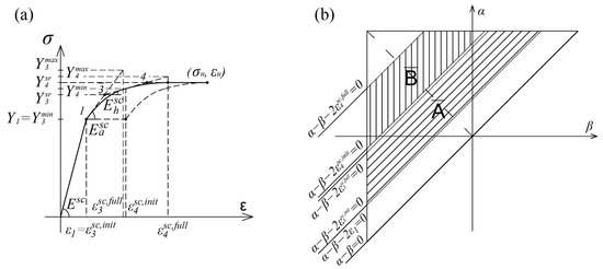
Figure 16.
(a) Skeleton curve; (b) Preisach triangle defining skeleton curve.
The Preisach’s function for skeleton curve is defined as follows:
where δ stands for the Dirac delta function and H for the Heaviside function.
The integration domains in Equation (7) represent the areas of the bands between the corresponding lines in a bounded triangle (Figure 16b) because the Preisach function exists only in these domains and otherwise is zero.
Domain represents the area between the lines and , while domain represents the area between the lines and .
5. Damage Modeling
Damage in steel elements may occur during forming processes [30] or under exploitative monotonic or cyclic loading. Defining damage under cyclic loading is a very complex problem. The material rupture limit σD at cyclic stress depends on the amount of energy accumulated in the material. The accumulation of deformation energy has material fatigue as a consequence. In the domain of elasticity for a large number of load cycles, fatigue is also noticeable. Damage under a small cycle number and large plastic deformations can be considered regardless of fatigue.
The drop in the stress–strain curve is modeled by two different Preisach models, regardless of the previous load history.
The problem of a large number of cycles may be resolved by applying cycle-counting methods. Verification of a model is conducted through comparison with the experimental results of monotonic tests. This approach is acceptable due to the equivalent shape of the stress–strain curve under monotonic and cyclic loading in the damage zone (Figure 11). The mechanical models defining damage under monotonic or cyclic loading are obtained by adaptation of the appropriate mechanical model (monotonic or cyclic).
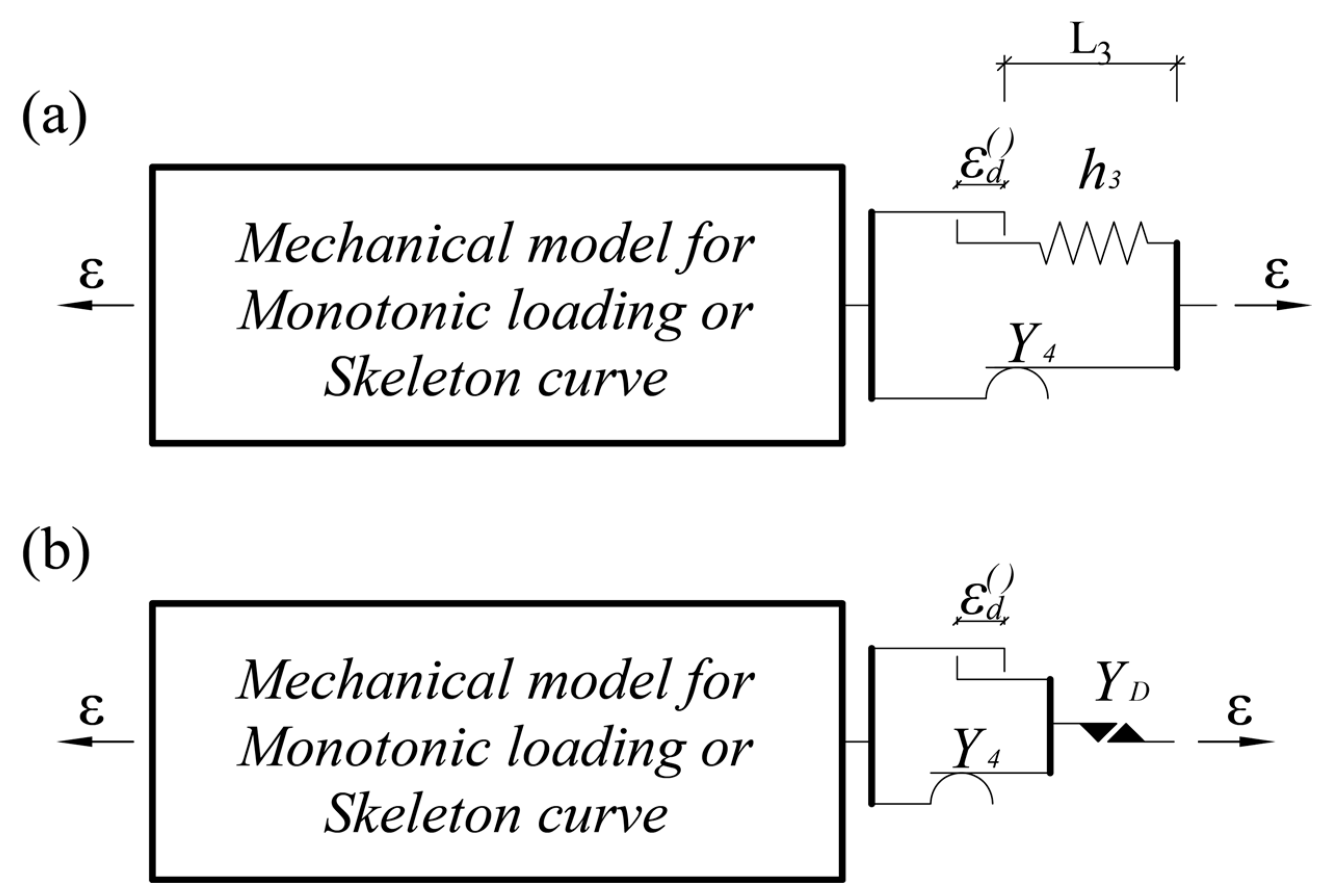
In this paper, two different Preisach models for defining damage are presented. Both use different approaches. PMD1 uses a spring with negative stiffness for defining drop in the stress–strain curve, while PMD2 uses a damage element with a rupture limit YD (Figure 17b).
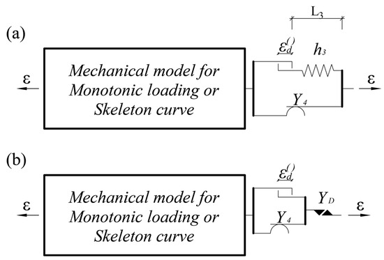
Figure 17.
Preisach model for defining damage: (a) with negative stiffness spring (PMD1); (b) with a damage element with rupture limit (PMD2).
PMD1 is described and verified through monotonic axial test loading [24], while the basic principles of PMD2 are defined in [28]. In both mechanical models, the last slip element Y4 (Figure 15a and [24]) is altered by a set of three distinct elements. The modified delay element, in both models, allows damage to the material under tension only.
The additional material characteristics are defined as follows:
where h3 is the negative stiffness of the last spring in PMD1, εd defines the length of the horizontal plateau after exceeding the yield strength Y4, and YD is the rupture limit in PMD2.
The YD must have an infinitesimal greater value than Y4 to allow the formation of a plateau of length εd on the stress–strain diagram.
The parallel connection of infinitely many mechanical models, shown in Figure 17a, delivers the polycrystalline material model PMD1. Using elements with different yield limits Yimin ≤ Yi ≤ Yimax and with different delay dilatations εd( )init ≤ ε( )d ≤ εd( )full, the expression for the total stress with damage (Figure 18a) is as follows:
where p(εd) represents the uniform distribution functions of delay dilatation εd( ):
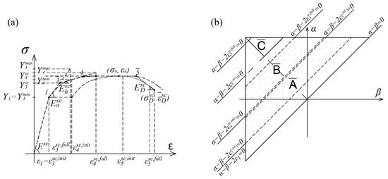
Figure 18.
(a) Stress–strain diagram of PMD1; (b) Preisach triangle defining PMD1.
The appropriate Preisach’s function is defined by (12).
where the last part of expression (12) denotes additional limit of domain of integration (Figure 18b). Domain represents the area between the lines , , and .
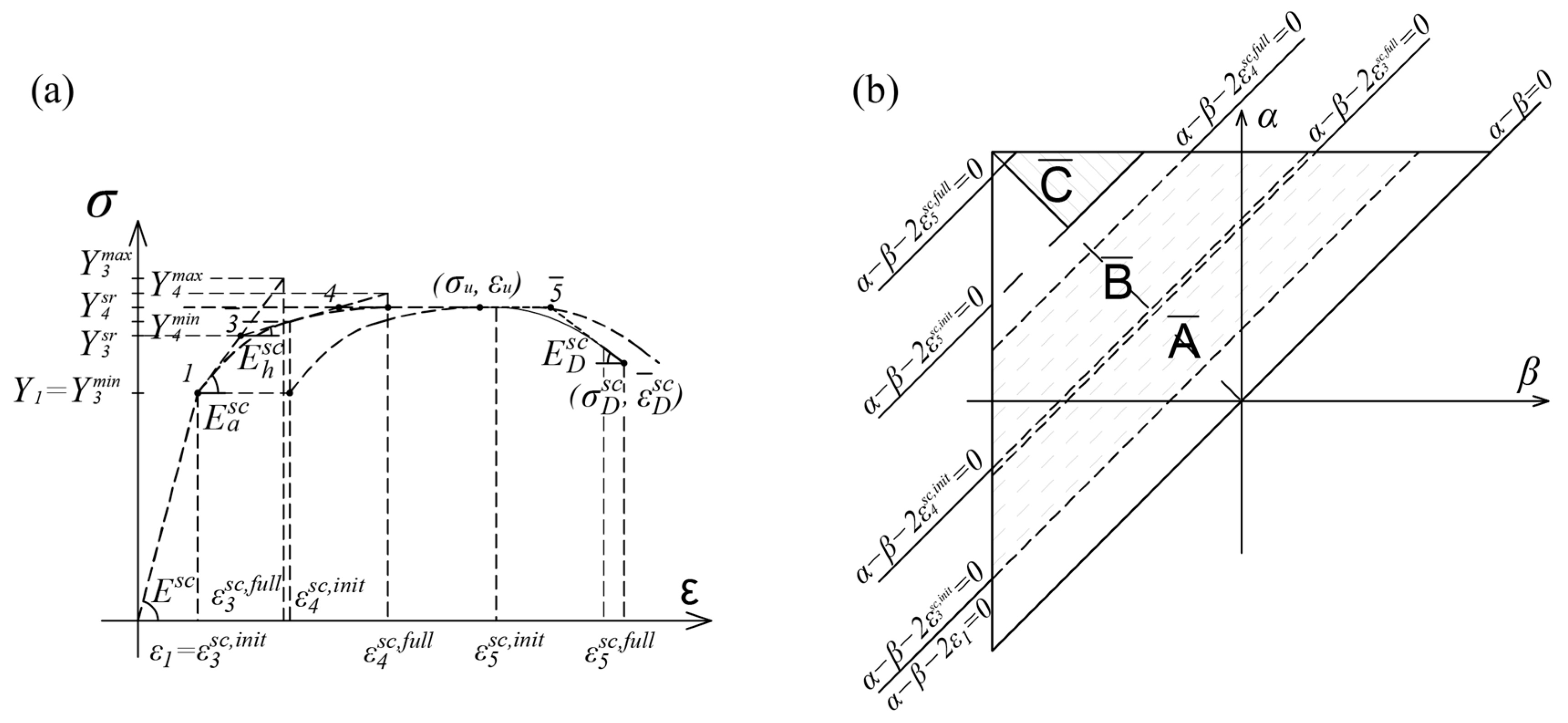
The polycrystalline material model PMD2 is created by connecting infinitely many mechanical models in parallel, as shown in Figure 17b. Mechanical models have different elastic yield strengths under fraction (). Due to the horizontal segment of the σ-ε diagram preceding the fracture, material crystals possess different fracture dilatations (), but constant stress under fracture YD. This phenomenon is achieved by varying the displacement length of the “delay” element εd in the mechanical model from Figure 17b.
The expression for the stress–strain curve with damage defined by PMD2 (Figure 19a) is as follows:
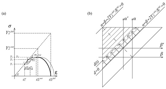
Figure 19.
(a) Stress–strain diagram of PMD2; (b) Preisach triangle defining PMD2.
The integration domain D defines the damage in the material and represents the area of the strip between the lines and . The D domain area of integration decreases with increasing deformation due to the translation of the lower limit. The horizontal line of the triangle also limits domain D. The vertical boundary in the triangle has no effect since damage occurs only under tension. The Preisach triangle defining the integration domain D is shown Figure 19b.
The scalar value of damage d, previously defined in [28], represents the ratio of the number of eliminated elements n and the total number of elements N in the material, determined by the following expression:
The value of d varies in limits 0 ≤ d ≤ 1, where the line represents the initiation of damage (d = 0) and the line denotes complete damage to the material (d = 1).
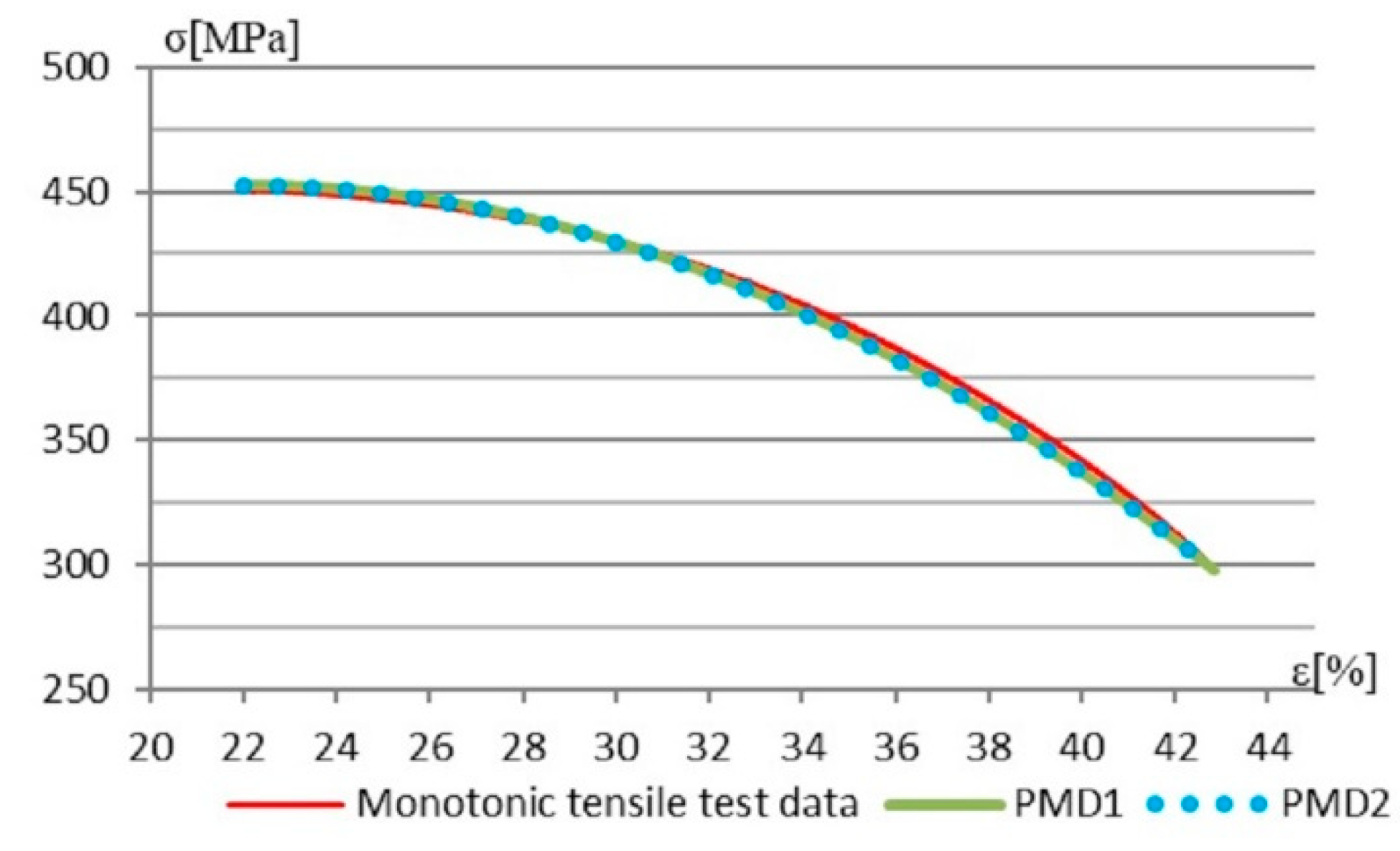
This section of the paper proposes damage modeling approaches for monotonic and cyclic loading based on existing models for monotonic loading. Verification of the presented Preisach models is conducted by comparing them with the experimental results of monotonic tests. The lack of experimental data for large-strain cyclic tests is due to issues with test samples buckling. As a result, models PMD1 and PMD2 can only be compared with test data from monotonic tensile tests in the damage zone (22–43%) (Figure 20).
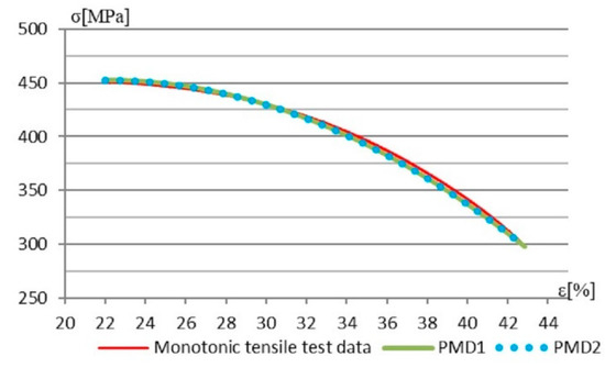
Figure 20.
Comparison of analytical and test results in sample damage zone.
Preisach models PMD1 and PMD2 showed remarkable resemblance in results. Also, models exhibited excellent agreement with the results of the monotonic tensile test in the damage zone.
For evaluating the quality of the presented models, we have employed the Root Mean Squared Error (RMSE). It represents the average difference between the predicted values and the actual values, helping to assess how accurately the model predicts the target variable.
Based on the conducted analysis, the RMSE for the first model PMD1 is 3.2516, and for the second model PMD2, it is 3.2651.
A lower RMSE indicates better predictive accuracy of the model, so we can conclude that the model PMD1 slightly better fits experimental data.
The damage modeling using PMD2 is more effortless because it requires fewer elements to describe the model for this type of steel. However, model PMD1 still provides a good solution for common engineering practice due to its more suitable geometrical representation.
6. Conclusions
The present paper focuses on an experimental investigation of the structural mild steel stress–strain characteristics under cyclic loading. The experimental program examined the correlation between the material monotonic and cyclic behavior, taking into account the effects of loading history. It is shown that the high cost of cyclic tests due to test setup limitations and specimen buckling issues may be overcome through the correlated performance of monotonic and cyclic test results.
In this paper, the correlation between these two types of behavior is established through the linkage of the hysteresis skeleton curve and monotonic loading curve. It is shown that a Lüders band phenomenon, the main characteristic of monotonic axial behavior, does not occur under cyclic loading. The trend line is formed using peak values of complete hysteresis loops obtained through cyclic testing. This curve based on experimental results is called the skeleton curve. It characterizes mild steel cyclic behavior and is modeled through a modified monotonic stress–strain curve. The monotonic stress–strain curve modification was achieved by excluding the yield plateau and adopting a faster stress increase in the material hardening zone for the same dilatation increase.
The new Preisach model defining the realistic behavior of mild steel under cyclic loading is developed using experimentally obtained correlations. The model is formed by upgrading the existing model for monotonic loading. The skeleton curve, as the main indicator of mild steel cyclic behavior, is described completely by the hysteresis model with material parameters obtained only through monotonic axial tests.
At the end of the paper, damage under a small number of cycles and large plastic deformations are modeled regardless of fatigue. Two different Preisach models’ extensions for defining damage are presented (PMD1 and PMD2). Both models’ extensions can be used to describe damage both under monotonic and cyclic loading.
The first model uses a spring with negative stiffness to define a drop in the stress–strain curve. Verification of a model is conducted through comparison with experimental results of monotonic tests. The second model using a damage element with a rupture limit YD is now verified through comparison with experimental and PMD1 data.
A comparison with experimental results of monotonic tests is acceptable due to the stress–strain curve form resemblance under monotonic and cyclic loading. This is also a consequence of the lack of experimental results of cyclic tests in the damage zone due to buckling problems and complicated test configuration. To overcome this drawback, it is possible to use a similar correlation between the two types of loadings outside the damage zone (adopting a double strain decrease in the damage zone).
Author Contributions
P.K. and Z.P. proposed the studied problem and applied the solution method; R.R. and P.K. conducted experimental investigation; A.R., D.Č. and P.K. conducted the theoretical derivation; P.K. and Z.P. proposed and conducted the theoretical derivation of damage models; N.V. and G.B. analyzed the results and wrote the manuscript. All authors have read and agreed to the published version of the manuscript.
Funding
This research received no external funding.
Data Availability Statement
The original contributions presented in the study are included in the article, further inquiries can be directed to the corresponding author.
Acknowledgments
Research presented in this paper was supported by the Ministry of Education, Science and Technological Development of Republic of Serbia, contract no. 451-03-65/2024-03/200155, realized by the Faculty of Technical Sciences in Kosovska Mitrovica, University of Pristina.
Conflicts of Interest
The authors declare no conflicts of interest.
References
- Zhang, Z.-J.; Chen, B.-S.; Bai, R.; Liu, Y.-P. Non-Linear Behavior and Design of Steel Structures: Review and Outlook. Buildings 2023, 13, 2111. [Google Scholar] [CrossRef]
- Xu, Z.; Rehman, U.U.; Mahmood, T.; Ahmmad, J.; Jin, Y. Assessment of Structural Systems to Design Earthquake Resistance Buildings by Employing Multi-Attribute Decision-Making Method Based on the Bipolar Complex Fuzzy Dombi Prioritized Aggregation Operators. Mathematics 2023, 11, 2226. [Google Scholar] [CrossRef]
- Nip, K.H.; Gardner, L.; Davies, C.M.; Elghazouli, A.Y. Extremely low cycle fatigue tests on structural carbon steel and stainless steel. J. Constr. Steel Res. 2010, 66, 96–110. [Google Scholar] [CrossRef]
- Dusicka, P.; Itani, A.M.; Buckle, I.G. Cyclic response of plate steels under large inelastic strains. J. Constr. Steel Res. 2007, 63, 156–164. [Google Scholar] [CrossRef]
- Zhou, F.; Chen, Y.; Wu, Q. Dependence of the cyclic response of structural steel on loading history under large inelastic strains. J. Constr. Steel Res. 2015, 104, 64–73. [Google Scholar] [CrossRef]
- Yoshida, F.; Uemori, T.; Fujiwara, K. Elastic–plastic behavior of steel sheets under in-plane cyclic tension–compression at large strain. Int. J. Plast. 2002, 18, 633–659. [Google Scholar] [CrossRef]
- Zhou, F.; Li, L. Experimental study on hysteretic behavior of structural stainless steels under cyclic loading. J. Constr. Steel Res. 2016, 122, 94–109. [Google Scholar] [CrossRef]
- Ucak, A.; Tsopelas, P. Accurate modeling of the cyclic response of structural components constructed of steel with yield plateau. Eng. Struct. 2012, 35, 272. [Google Scholar] [CrossRef]
- Chang, K.-C.; Lee, G.C. Constitutive Relations of Structural Steel under Nonproportional Loading. J. Eng. Mech. 1986, 112, 806–820. [Google Scholar] [CrossRef]
- ISO 12106; Metallic Materials—Fatigue Testing—Axial Strain Controlled Method. CEN: Brussels, Belgium, 2017.
- ASTM. Standard Test Methods for Tension Testing of Metallic Materials; ASTM International: West Conshohocken, NY, USA, 2021. [Google Scholar] [CrossRef]
- GB/T 228.1-2021; Chinese Standard. Metallic Materials-Tensile Testing—Part: 1 Method of Test at Room Temperature. The Chinese National Standard: Beijing, China, 2008.
- DIN EN ISO 6892-1; Metallic Materials—Tensile Testing—Part 1: Method of Test at Room Temperature. EN Standards: Plzen, Czech Republic, 2020. Available online: https://www.en-standard.eu/din-en-iso-6892-1-metallic-materials-tensile-testing-part-1-method-of-test-at-room-temperature-iso-6892-1-2019/ (accessed on 28 January 2022).
- Dahl, P.R. Solid Friction Damping of Mechanical Vibrations. AIAA J. 1976, 14, 1675–1682. [Google Scholar] [CrossRef]
- Jiles, D.C.; Atherton, D.L. Theory of ferromagnetic hysteresis. J. Magn. Magn. Mater. 1986, 61, 48–60. [Google Scholar] [CrossRef]
- Sucuoglu, H.; Erberik, M.A. Energy-based hysteresis and damage models for deteriorating systems. Earthq. Eng. Struct. Dyn. 2003, 33, 69–88. [Google Scholar] [CrossRef]
- Jayawardhana, B.; Logemann, H.; Ryan, E.P. PID control of second-order systems with hysteresis. Int. J. Control 2003, 81, 1331–1342. [Google Scholar] [CrossRef]
- Solovyov, A.M.; Selvesyuk, N.I.; Kosyanchuk, V.V.; Zybin, E.Y. A Model of a Universal Neural Computer with Hysteresis Dynamics for Avionics Problems. Mathematics 2022, 10, 2390. [Google Scholar] [CrossRef]
- Semenov, M.E.; Borzunov, S.V.; Meleshenko, P.A.; Lapin, A.V. A Model of Optimal Production Planning Based on the Hysteretic Demand Curve. Mathematics 2022, 10, 3262. [Google Scholar] [CrossRef]
- Preisach, F. Über die magnetische Nachwirkung. Z. Phys. 1935, 94, 277–302. [Google Scholar] [CrossRef]
- Krasnoselskii, M.; Pokrovskii, A. Systems with Hysteresis; Nauka: Moscow, Russia, 1983. [Google Scholar]
- Mörée, G.; Leijon, M. Review of Play and Preisach Models for Hysteresis in Magnetic Materials. Materials 2023, 16, 2422. [Google Scholar] [CrossRef]
- Mendes, L.A.M.; Castro, L.M.S.S. A simplified reinforcing steel model suitable for cyclic loading including ultra-low-cycle fatigue effects. Eng. Struct. 2014, 68, 155–164. [Google Scholar] [CrossRef]
- Knežević, P.; Šumarac, D.; Perović, Z.; Dolićanin, Ć.; Burzić, Z. A Preisach Model for Monotonic Tension Response of Structural Mild Steel with Damage. Period. Polytech. Civ. Eng. 2020, 64, 296–303. [Google Scholar] [CrossRef]
- Iwan, W.D. On a Class of Models for the Yielding Behavior of Continuous and Composite Systems. J. Appl. Mech. 1967, 34, 612–617. [Google Scholar] [CrossRef]
- Lubarda, A.V.; Sumarac, D.; Krajcinovic, D. Hysteretic response of ductile materials subjected to cyclic loads. Recent Adv. Damage Mech. Plast. ASME Publ. AMD 1992, 123, 145–157. [Google Scholar]
- Lubarda, V.A.; Sumarac, D.; Krajcinovic, D. Preisach model and hysteretic behaviour of ductile materials. Eur. J. Mech. A Solids 1993, 12, 445–470. [Google Scholar]
- Šumarac, D.; Perovic, Z. Cyclic plasticity of trusses. Arch. Appl. Mech. 2014, 85, 1513–1526. [Google Scholar] [CrossRef]
- Šumarac, D.; Petrašković, Z. Hysteretic behavior of rectangular tube (box) sections based on Preisach model. Arch. Appl. Mech. 2012, 82, 1663–1673. [Google Scholar] [CrossRef]
- Said, L.B.; Allouch, M.; Wali, M.; Dammak, F. Numerical Formulation of Anisotropic Elastoplastic Behavior Coupled with Damage Model in Forming Processes. Mathematics 2023, 11, 204. [Google Scholar] [CrossRef]


Disclaimer/Publisher’s Note: The statements, opinions and data contained in all publications are solely those of the individual author(s) and contributor(s) and not of MDPI and/or the editor(s). MDPI and/or the editor(s) disclaim responsibility for any injury to people or property resulting from any ideas, methods, instructions or products referred to in the content. |
© 2024 by the authors. Licensee MDPI, Basel, Switzerland. This article is an open access article distributed under the terms and conditions of the Creative Commons Attribution (CC BY) license (https://creativecommons.org/licenses/by/4.0/).