H_∞ Filtering of Mean Field Stochastic Differential Systems

Abstract

This paper addresses the $H_{\infty }$ filtering problem for mean field stochastic differential systems that involve both state-dependent and disturbance-dependent noise. We assume that the state as well as the measurement output is distracted by an uncertain exogenous disturbance. Firstly, a sufficient condition for the stochastic-bounded real lemma is given. Next, $H_{\infty }$ filtering, which is built upon a stochastic-bounded real lemma, is put forward by two linear matrix inequalities. Furthermore, the validation of the theoretical analysis is demonstrated with two examples.

1. Introduction

When there are a large number of individuals in a system and each one follows a certain stochastic process, interactions between these individuals can be simplified at the macro level as the mean field, and then the system can be modeled using the “mean field” term. That is, the key idea for the mean field stochastic system is to use mean field approximation to handle complex interactions. Research on mean field stochastic systems began in the early 20th century; see [1] and the references therein. Up to now, there have been considerable theoretical and practical achievements in its development. Recently, mean field control and filtering theories have garnered increasing interested in the fields of mathematics and control. The stochastic maximum principle has been explored, and the necessary conditions for optimality have been given. In [2,3], Markowitz mean variance portfolio selection and a class of mean field linear quadratic problems were dealt with to take advantage of the stochastic maximum principle. Grounded in the mean field stochastic maximum principle, ref. [4] used variational and decoupling methods to discuss the finite horizon linear quadratic optimal control problem of stochastic mean field differential systems. Moreover, the linear feedback gain of the optimal control was obtained with the help of the solutions of two coupled differential Riccati equations. Afterward, ref. [5] expanded the above conclusion to the infinite horizon case. Furthermore, ref. [6] has considered the linear quadratic optimal control problem for discrete-time mean field stochastic systems with Markov jump parameters. Other significant works concerning the mean field optimal control problem can be found in [7,8,9,10,11]. In addition, $H_2/H_{\infty }$ control has been broadly investigated. For example, ref. [12] introduced $H_2/H_{\infty }$ control for discrete-time mean field systems with Poisson jump. Ref. [13] studied the $H_2/H_{\infty }$ control of mean field stochastic differential systems with $(x,u,v)$-dependent noise.

In practical engineering, the state of a system is often disturbed by exogenous noise. How to obtain the estimation of the linear combination of system states by utilizing output measurements is a basic matter in system theory. The Kalman filter (or extended Kalman filter) is considered to be one of the most powerful estimation methods when the exogenous disturbance is stationary Gaussian white noise [14]. On the other hand, in the case that the statistical characteristics of the external disturbance are unascertained, Kalman filtering is no longer effective. Notice that $H_{\infty }$ filtering can be used to handle a case in which external disturbances have bounded energy rather than a Gaussian distribution. More specifically, the $H_{\infty }$ filtering problem involves designing an estimator that estimates the unknown state combination through measurement outputs, and ensures that for any prescribed level $\gamma >0$, the $H_{\infty }$ gain is always less than $\gamma$. To estimate the state for a class of nonlinear discrete-time systems, [15] developed the fuzzy filtering design. Additionally, $H_{\infty }$ control and filtering for discrete-time stochastic systems with multiplicative noise was considered in [16]. Ref. [17] discussed robust $H_{\infty }$ filtering for stationary continuous-time stochastic uncertainty systems. The authors of [18,19] tackled the robust $H_{\infty }$ filtering problem for stochastic uncertain systems and nonlinear stochastic systems, respectively. Ref. [20] addressed dynamic sum-based event-triggered $H_{\infty }$ filtering for a class of networked T-S fuzzy wind turbine systems. It should be conveyed that the research on $H_{\infty }$ filtering for systems represented by It$\widehat{o}$ stochastic differential equations receives widespread attention and achieves great results, but rarely on the mean field type. Ref. [21] discussed annular finite-time $H_{\infty }$ filtering. But there is no relevant conclusion on the infinite horizon case.

This paper focuses on the $H_{\infty }$ state estimation of continuous-time mean field stochastic systems with exogenous disturbance noise. The main contributions of this paper are as follows: First, the infinite horizon stochastic bounded real lemma is set up. It shows that for internally stable systems, the $H_{\infty }$ performance index $J_s<0$ relies on the viability of some linear matrix inequalities. Second, a filter is constructed such that the $H_{\infty }$ gain is less than a prescribed level $\gamma >0$, while the augmented system is ensured to be internally stable. The remainder is divided into four parts: In Section 2, the design problem is stated and preliminaries are elaborated; the proof of the mean field stochastic-bounded real lemma is included in Section 3, and consequently, the $H_{\infty }$ filter can be designed based on the solution of two linear matrix inequalities; Two examples are offered in Section 4 to validate the results obtained; In Section 5, this paper ends with some concluding remarks.

2. Preliminaries

We utilize the following notations for convenience:

• ${\mathbb{R}}^m$ is the m-dimensional real vector space that has the usual inner product;
• I represents the identity matrix;
• $X\ge 0$ $(X>0)$ means that X is a positive semidefinite (positive definite) matrix;
• $X^{\top }$ denotes the transpose of a matrix or vector X;
• E is the expectation operator;
• ${\mathcal{L}}_{\mathcal{F}}^2([0,T],{\mathbb{R}}^l)$ stands for the space of nonanticipative stochastic processes $y_t\in {\mathbb{R}}^l$ associated with an increasing $\sigma$-algebras ${\mathcal{F}}_t$ satisfying $E{\int }_0^T{\parallel y_t\parallel }^{2}dt<\infty$;
• $H_n\left(\mathbb{R}\right)$ is the set of all $n\times n$ real symmetric matrices.

Next, we make the following assumption:

Assumption 1.

All matrices included in this paper are real constants.

Consider the below mean field stochastic differential system:

$$\left\{\begin{array}{cc}\hfill d{x}_t& =[A{x}_t+\overline{A}E{x}_t+B{v}_t+\overline{B}E{v}_t]dt+[C{x}_t+\overline{C}E{x}_t+D{v}_t+\overline{D}E{v}_t]dw,\hfill \\ \hfill y_t& =K{x}_t+F{v}_t,\hfill \\ \hfill z_t& =L{x}_t+\overline{L}E{x}_t,\hfill \end{array}\right.$$

(1)

where $x_t\in {\mathbb{R}}^n$ is the system state, $x_0={\zeta }_0$ is the initial value, $v\in {\mathcal{L}}_{\mathcal{F}}^2({\mathbb{R}}_{+},{\mathbb{R}}^l)$ is the exogenous disturbance signal, $y_t\in {\mathbb{R}}^r$ is the measurement output, and $z_t\in {\mathbb{R}}^m$ is the signal that needs to be estimated. $w_t$ is a normal scalar Wiener process, determined in the probability space $(\mathsf{\Omega }$, $\mathbf{F}$, $\mathbf{P})$ with regard to an increasing family ${\left\{{\mathcal{F}}_t\right\}}_{t>0}$.

Take the filter equation

$$\left\{\begin{array}{cc}\hfill d{\widehat{x}}_t& =[A_f{\widehat{x}}_t+{\overline{A}}_{f}E{\widehat{x}}_t]dt+B_{f}d{y}_t+{\overline{B}}_{f}dE{y}_t,\hfill \\ \hfill {\widehat{x}}_0& =0,\hfill \\ \hfill {\widehat{z}}_t& =L_f{\widehat{x}}_t+{\overline{L}}_{f}E{\widehat{x}}_t\hfill \end{array}\right.$$

(2)

as the estimation of $z_t$, where ${\widehat{x}}_t\in {\mathbb{R}}^n$, ${\widehat{z}}_t\in {\mathbb{R}}^m$.

Let

$${\xi }_t^{\top }=\left[\begin{array}{cc}{x}_t^{\top }& {\widehat{x}}_t^{\top }\end{array}\right],$$

$${\tilde{z}}_t=z_t-{\widehat{z}}_t.$$

Upon the above indication, the equation of the filter estimation error ${\tilde{z}}_t$ can be built,

$$\left\{\begin{array}{cc}\hfill d{\xi }_t& =[A_m{\xi }_t+{\overline{A}}_{m}E{\xi }_t+B_m{v}_t+{\overline{B}}_{m}E{v}_t]dt+[C_m{\xi }_t+{\overline{C}}_{m}E{\xi }_t+D_m{v}_t+{\overline{D}}_{m}E{v}_t]dw,\hfill \\ \hfill {\tilde{z}}_t& =L_m{\xi }_t+{\overline{L}}_{m}E{\xi }_t,\hfill \end{array}\right.$$

(3)

where

$$\begin{array}{c}{A}_m=\left[\begin{array}{cc}A& 0\\ B_{f}K& A_f\end{array}\right],{\overline{A}}_m=\left[\begin{array}{cc}\overline{A}& 0\\ {\overline{B}}_{f}K& {\overline{A}}_f\end{array}\right],B_m=\left[\begin{array}{c}B\\ B_{f}F\end{array}\right],{\overline{B}}_m=\left[\begin{array}{c}\overline{B}\\ {\overline{B}}_{f}F\end{array}\right],\hfill \\ C_m=\left[\begin{array}{cc}C& 0\\ 0& 0\end{array}\right],{\overline{C}}_m=\left[\begin{array}{cc}\overline{C}& 0\\ 0& 0\end{array}\right],D_m=\left[\begin{array}{c}D\\ 0\end{array}\right],{\overline{D}}_m=\left[\begin{array}{c}\overline{D}\\ 0\end{array}\right],\hfill \\ L_m=\left[\begin{array}{cc}L& -L_f\end{array}\right],{\overline{L}}_m=\left[\begin{array}{cc}\overline{L}& -{\overline{L}}_f\end{array}\right].\hfill \end{array}$$

(4)

Similarly, in view of (3) and taking expectations, it can be established that:

$$\left\{\begin{array}{cc}\hfill dE{\xi }_t& =[(A_m+{\overline{A}}_m)E{\xi }_t+(B_m+{\overline{B}}_m)E{v}_t]dt,\hfill \\ \hfill E{\xi }_0^{\top }& =\left[\begin{array}{cc}E{\zeta }_0^{\top }& 0\end{array}\right],\hfill \\ \hfill E{\tilde{z}}_t& =(L_m+{\overline{L}}_m)E{\xi }_t,\hfill \end{array}\right.$$

Obviously, ${\xi }_t=E{\xi }_t+({\xi }_t-E{\xi }_t)$, with $E{\xi }_t$ and ${\xi }_t-E{\xi }_t$ being orthogonal in the sense that

$$E\left[E{\xi }_t{({\xi }_t-E{\xi }_t)}^{\top }\right]=0.$$

${\xi }_t-E{\xi }_t$ can be introduced as follows:

$$\left\{\begin{array}{cc}\hfill d({\xi }_t-E{\xi }_t)& =[A_m({\xi }_t-E{\xi }_t)+B_m(v_t-E{v}_t)]dt\hfill \\ \hfill & +[C_m({\xi }_t-E{\xi }_t)+(C_m+{\overline{C}}_m)E{\xi }_t+D_m(v_t-E{v}_t)+(D_m+{\overline{D}}_m)E{v}_t]dw,\hfill \\ \hfill {({\xi }_0-E{\xi }_0)}^{\top }& =\left[\begin{array}{cc}{({\zeta }_0-E{\zeta }_0)}^{\top }& 0\end{array}\right],\hfill \\ \hfill ({\tilde{z}}_t-E{\tilde{z}}_t)& =L_m({\xi }_t-E{\xi }_t).\hfill \end{array}\right.$$

For any prescribed disturbance attenuation level $\gamma >0$, we define an infinite horizon $H_{\infty }$ performance index:

$$J_s=\parallel {\tilde{z}}_t{\parallel }^2-{\gamma }^2{\parallel v_t\parallel }^2,t>0.$$

For system (3), the definition and the proposition given below are very essential.

Definition 1.

According to Ref. [22], if there exists a positive constant ε satisfying $E{\int }_0^{\infty }\parallel {\xi }_t{\parallel }^{2}dt\le \epsilon {\parallel {\zeta }_0\parallel }^2$, then we say that system (3) is internally stable, where ${\xi }_t$ is the free trajectory of (3) (i.e., $v_t=0$) starting at ${\zeta }_0$.

Proposition 1.

According to Ref. [22], if, for any negative definite matrices $R_m,S_m\in H_n\left(\mathbb{R}\right)$ there exist $P_m,Q_m\in H_n\left(\mathbb{R}\right)$ with $P_m>0$, $Q_m>0$ such that

$$\left\{\begin{array}{c}{P}_m{A}_m+A_m^{\top }{P}_m+C_m^{\top }{P}_m{C}_m=R_m,\hfill \\ Q_m(A_m+{\overline{A}}_m)+{(A_m+{\overline{A}}_m)}^{\top }{Q}_m+{(C_m+{\overline{C}}_m)}^{\top }{P}_m(C_m+{\overline{C}}_m)=S_m,\hfill \end{array}\right.$$

then system (3) is internally stable.

For system (1), the infinite horizon $H_{\infty }$ filtering estimation problem can be formulated as follows:

Given $\gamma >0$, find a linear filter with the form (2) such that

(i) 

$J_s<0$ for all nonzero $v\in {\mathcal{L}}_{\mathcal{F}}^2({\mathbb{R}}_{+},{\mathbb{R}}^l)$ with ${\zeta }_0=0$;

(ii) 

System (3) is internally stable.

3. ${\mathit{H}}_{\mathbf{\infty }}$ Filtering

This section begins with the mean field stochastic-bounded real lemma, which is an important foundation for carrying out $H_{\infty }$ filtering estimation.

Below, we first recall Schur’s complement lemma.

Lemma 1.

According to Ref. [23] (Schur’s complement lemma), for matrices $M_{11}=M_{11}^{\top }$, $M_{12}=M_{21}^{\top }$ and $M_{22}=M_{22}^{\top }$ with suitable dimensions, the following two conditions are equivalent:

(1) 

$\left[\begin{array}{cc}{M}_{11}& M_{12}\\ M_{21}& M_{22}\end{array}\right]<0$;

(2) 

$M_{11}<0$, $M_{22}-M_{21}{M}_{11}^{-1}{M}_{12}<0$.

Define the finite horizon quadratic cost functional,

$$J_s(T,{\zeta }_0,v)=E{\int }_0^T[\parallel {\tilde{z}}_t{\parallel }^2-{\gamma }^2\parallel v_t{\parallel }^2]dt,$$

where ${\xi }_t$ denotes the solution of (3) with ${\xi }_0={\zeta }_0$ and the hypothesis of $v_t\in {\mathcal{L}}_{\mathcal{F}}^2({\mathbb{R}}_{+},{\mathbb{R}}^l)$, and ${\tilde{z}}_t$ is the corresponding output.

For $J_s(T,{\zeta }_0,v)$, the following lemma can be derived from [22] directly.

Lemma 2.

Consider system (3). For $T>0$, assume that $P:[0,T]\mapsto H_n\left(\mathbb{R}\right)$ and $Q:[0,T]\mapsto H_n\left(\mathbb{R}\right)$ are continuously differentiable; then, for any ${\zeta }_0\in {\mathbb{R}}^n$ and $v_t\in {\mathcal{L}}_{\mathcal{F}}^2([0,T],{\mathbb{R}}^l)$, we have

$$\begin{array}{c}\hfill \begin{array}{cc}\hfill J_s(T,{\zeta }_0,v)& =E{\int }_0^T\left[{({\xi }_t-E{\xi }_t)}^{\top }{\dot{P}}_t({\xi }_t-E{\xi }_t)\right]dt+{\int }_0^T\left[E{\xi }_t^{\top }{\dot{Q}}_{t}E{\xi }_t\right]dt\hfill \\ & +E{\int }_0^T{\left[\begin{array}{c}{\xi }_t-E{\xi }_t\\ v_t-E{v}_t\end{array}\right]}^{\top }G\left(P_t\right)\left[\begin{array}{c}{\xi }_t-E{\xi }_t\\ v_t-E{v}_t\end{array}\right]dt+{\int }_0^T{\left[\begin{array}{c}E{\xi }_t\\ E{v}_t\end{array}\right]}^{\top }N(P_t,Q_t)\left[\begin{array}{c}E{\xi }_t\\ E{v}_t\end{array}\right]dt\hfill \\ & +E{({\xi }_0-E{\xi }_0)}^{\top }{P}_0({\xi }_0-E{\xi }_0)+E{\xi }_0^{\top }{Q}_{0}E{\xi }_0\hfill \\ & -E{({\xi }_T-E{\xi }_T)}^{\top }{P}_T({\xi }_T-E{\xi }_T)-E{\xi }_T^{\top }{Q}_{T}E{\xi }_T,\hfill \end{array}\end{array}$$

where

$$\tilde{A}=(A_m+{\overline{A}}_m),\tilde{B}=(B_m+{\overline{B}}_m),\tilde{C}=(C_m+{\overline{C}}_m),\tilde{D}=(D_m+{\overline{D}}_m),\tilde{L}=(L_m+{\overline{L}}_m),$$

(5)

$$G\left(P_t\right)=\left[\begin{array}{cc}{A}_m^{\top }{P}_t+P_t{A}_m+C_m^{\top }{P}_t{C}_m+L_m^{\top }{L}_m& P_t{B}_m+C_m^{\top }{P}_t{D}_m\\ B_m^{\top }{P}_t+D_m^{\top }{P}_t{C}_m& D_m^{\top }{P}_t{D}_m-{\gamma }^2{I}_l\end{array}\right],$$

(6)

$$N(P_t,Q_t)=\left[\begin{array}{cc}{\tilde{A}}^{\top }{Q}_t+Q_t\tilde{A}+{\tilde{C}}^{\top }{P}_t\tilde{C}+{\tilde{L}}^{\top }\tilde{L}& Q_t\tilde{B}+{\tilde{C}}^{\top }{P}_t\tilde{D}\\ {\tilde{B}}^{\top }{Q}_t+{\tilde{D}}^{\top }{P}_t\tilde{C}& {\tilde{D}}^{\top }{P}_t\tilde{D}-{\gamma }^2{I}_l\end{array}\right].$$

(7)

Now, we are ready to present the mean field stochastic-bounded real lemma.

Theorem 1.

(Stochastic Bounded Real Lemma) For a given disturbance attenuation $\gamma >0$, if $G\left(P\right)<0$ and $N(P,Q)<0$ hold for $(P,Q)$ with $P>0$, $Q>0$, then system (3) is internally stable, as is the $H_{\infty }$ filtering performance $J_s<0$.

Proof. 

Considering that $G\left(P_t\right)<0$ and $N(P_t,Q_t)<0$, it can be drawn from the lemma 1 that

$$A_m^{\top }P+P{A}_m+C_m^{\top }P{C}_m+L_m^{\top }{L}_m<0,$$

and

$${\tilde{A}}^{\top }Q+Q\tilde{A}+{\tilde{C}}^{\top }P\tilde{C}+{\tilde{L}}^{\top }\tilde{L}<0.$$

Therefore, we conclude that

$$A_m^{\top }P+P{A}_m+C_m^{\top }P{C}_m<0,$$

and

$${\tilde{A}}^{\top }Q+Q\tilde{A}+{\tilde{C}}^{\top }P\tilde{C}<0.$$

Thus, according to Proposition 1, system (3) is internally stable.

Next, we prove that $J_s<0$. In Lemma 2, by setting ${\zeta }_0=0$, $P_t=P$ and $Q_t=Q$, we obtain the following:

$$\begin{array}{c}\hfill \begin{array}{cc}\hfill J_s(T,0,v)& =E{\int }_0^T[\parallel {\tilde{z}}_t{\parallel }^2-{\gamma }^2\parallel v_t{\parallel }^2]dt\hfill \\ & =E{\int }_0^T{\left[\begin{array}{c}{\xi }_t-E{\xi }_t\\ v_t-E{v}_t\end{array}\right]}^{\top }G\left(P\right)\left[\begin{array}{c}{\xi }_t-E{\xi }_t\\ v_t-E{v}_t\end{array}\right]dt+{\int }_0^T{\left[\begin{array}{c}E{\xi }_t\\ E{v}_t\end{array}\right]}^{\top }N(P,Q)\left[\begin{array}{c}E{\xi }_t\\ E{v}_t\end{array}\right]dt\hfill \\ & -E{({\xi }_T-E{\xi }_T)}^{\top }P({\xi }_T-E{\xi }_T)-E{\xi }_T^{\top }QE{\xi }_T.\hfill \end{array}\end{array}$$

Due to $G\left(P\right)<0$ and $N(P,Q)<0$, we can choose a sufficiently small $\epsilon >0$ such that $G\left(P\right)\le -{\epsilon }^2{I}_{n+l}$, $N(P,Q)\le -{\epsilon }^2{I}_{n+l}$. Therefore, we have

$$\begin{array}{c}\hfill \begin{array}{cc}\hfill J_s(T,0,v)& =E{\int }_0^T[\parallel {\tilde{z}}_t{\parallel }^2-{\gamma }^2\parallel v_t{\parallel }^2]dt\hfill \\ & \le E{\int }_0^T-{\epsilon }^2[\parallel {\xi }_t-E{\xi }_t{\parallel }^2+\parallel v_t-E{v}_t{\parallel }^2]dt+{\int }_0^T-{\epsilon }^2[\parallel E{\xi }_t{\parallel }^2+\parallel E{v}_t{\parallel }^2]dt\hfill \\ & -E{({\xi }_T-E{\xi }_T)}^{\top }P({\xi }_T-E{\xi }_T)-E{\xi }_T^{\top }QE{\xi }_T\hfill \\ & \le E{\int }_0^T-{\epsilon }^2[\parallel {\xi }_t-E{\xi }_t{\parallel }^2+\parallel v_t-E{v}_t{\parallel }^2]dt+{\int }_0^T-{\epsilon }^2[\parallel E{\xi }_t{\parallel }^2+\parallel E{v}_t{\parallel }^2]dt\hfill \\ & \le -{\epsilon }^{2}E{\int }_0^T{\parallel v_t\parallel }^{2}dt.\hfill \end{array}\end{array}$$

(8)

Letting $T\to \infty$ in (8), it follows that

$$\begin{array}{c}\hfill \begin{array}{c}\hfill J_s=E{\int }_0^{\infty }[\parallel {\tilde{z}}_t{\parallel }^2-{\gamma }^2\parallel v_t{\parallel }^2]dt\le -{\epsilon }^{2}E{\int }_0^{\infty }{\parallel v_t\parallel }^{2}dt<0\end{array}\end{array}$$

for all nonzero $v_t\in {\mathcal{L}}_{\mathcal{F}}^2({\mathbb{R}}_{+},{\mathbb{R}}^l)$ with ${\zeta }_0=0$, which ends the proof. □

Based on Theorem 1, the infinite horizon $H_{\infty }$ filtering estimation problem can be solved.

Theorem 2.

If the following linear matrix inequalities,

$$\left[\begin{array}{cccccc}{A}^{\top }{P}_{11}+P_{11}A& K^{\top }{Z}_1^{\top }& P_{11}B+C^{\top }{P}_{11}D& C^{\top }{P}_{11}& 0& L^{\top }\\ Z_{1}K& Z+Z^{\top }& Z_{1}F& 0& 0& -L_f^{\top }\\ B^{\top }{P}_{11}+D^{\top }{P}_{11}C& F^{\top }{Z}_1^{\top }& D^{\top }{P}_{11}D-{\gamma }^{2}I& 0& 0& 0\\ P_{11}C& 0& 0& -P_{11}& 0& 0\\ 0& 0& 0& 0& -P_{22}& 0\\ L& -L_f& 0& 0& 0& -I\end{array}\right]<0,$$

(9)

and

$$\left[\begin{array}{cccccc}{\widehat{A}}^{\top }{Q}_{11}+Q_{11}\widehat{A}& K^{\top }{\widehat{Z_1}}^{\top }& Q_{11}\widehat{B}+{\widehat{C}}^{\top }{P}_{11}\widehat{D}& {\widehat{C}}^{\top }{P}_{11}& 0& {\widehat{L}}^{\top }\\ \widehat{Z_1}K& \widehat{Z}+{\widehat{Z}}^{\top }& \widehat{Z_1}F& 0& 0& -{\widehat{L}}_f^{\top }\\ {\widehat{B}}^{\top }{Q}_{11}+{\widehat{D}}^{\top }{P}_{11}\widehat{C}& F^{\top }{\widehat{Z_1}}^{\top }& {\widehat{D}}^{\top }{P}_{11}\widehat{D}-{\gamma }^{2}I& 0& 0& 0\\ P_{11}\widehat{C}& 0& 0& -P_{11}& 0& 0\\ 0& 0& 0& 0& -P_{22}& 0\\ \widehat{L}& -{\widehat{L}}_f& 0& 0& 0& -I\end{array}\right]<0$$

(10)

have solutions $P_{11}>0$, $P_{22}>0$, $Q_{11}>0$, $L_f$, ${\overline{L}}_f$, $Z_1$, ${\overline{Z}}_1$, Z and $\overline{Z}$, then (3) is internally stable and $J_s<0$, where

$$\begin{array}{c}\hfill \begin{array}{cc}\hfill \widehat{A}& =(A+\overline{A}),\widehat{B}=(B+\overline{B}),\widehat{C}=(C+\overline{C}),\widehat{D}=(D+\overline{D}),\hfill \\ \hfill \widehat{L}& =(L+\overline{L}),{\widehat{L}}_f=(L_f+{\overline{L}}_f),\widehat{Z}=(Z+\overline{Z}),\widehat{Z_1}=(Z_1+\overline{Z_1}).\hfill \end{array}\end{array}$$

(11)

Moreover, $H_{\infty }$ filtering can be formulated as

$$\left\{\begin{array}{c}d{\widehat{x}}_t=[P_{22}^{-1}Z{\widehat{x}}_t+P_{22}^{-1}\overline{Z}E{\widehat{x}}_t]dt+P_{22}^{-1}{Z}_{1}d{y}_t+P_{22}^{-1}{\overline{Z}}_{1}dE{y}_t,\hfill \\ {\widehat{z}}_t=L_f{\widehat{x}}_t+{\overline{L}}_{f}E{\widehat{x}}_t.\hfill \end{array}\right.$$

(12)

Proof. 

By Lemma 1, (6) and (7) are equivalent to

$$\left[\begin{array}{cccc}{A}_m^{\top }P+P{A}_m& P{B}_m+C_m^{\top }P{D}_m& C_m^{\top }P& L_m^{\top }\\ B_m^{\top }P+D_m^{\top }P{C}_m& D_m^{\top }P{D}_m-{\gamma }^{2}I& 0& 0\\ P{C}_m& 0& -P& 0\\ L_m& 0& 0& -I\end{array}\right]$$

(13)

and

$$\left[\begin{array}{cccc}{\tilde{A}}^{\top }Q+Q\tilde{A}& Q\tilde{B}+{\tilde{C}}^{\top }P\tilde{D}& {\tilde{C}}^{\top }P& {\tilde{L}}^{\top }\\ {\tilde{B}}^{\top }Q+{\tilde{D}}^{\top }P\tilde{C}& {\tilde{D}}^{\top }P\tilde{D}-{\gamma }^{2}I& 0& 0\\ P\tilde{C}& 0& -P& 0\\ \tilde{L}& 0& 0& -I\end{array}\right],$$

(14)

respectively. Take $P=diag(P_{11},P_{22})$ and $Q=diag(Q_{11},Q_{22})$. Substituting (4), (5), (11) into (13) and (14), we have

$$\left[\begin{array}{cccccc}{A}^{\top }{P}_{11}+P_{11}A& K^{\top }{B}_f^{\top }{P}_{22}& P_{11}B+C^{\top }{P}_{11}D& C^{\top }{P}_{11}& 0& L^{\top }\\ P_{22}{B}_{f}K& A_f^{\top }{P}_{22}+P_{22}{A}_f& P_{22}{B}_{f}F& 0& 0& -L_f^{\top }\\ B^{\top }{P}_{11}+D^{\top }{P}_{11}C& F^{\top }{B}_f^{\top }{P}_{22}& D^{\top }{P}_{11}D-{\gamma }^{2}I& 0& 0& 0\\ P_{11}C& 0& 0& -P_{11}& 0& 0\\ 0& 0& 0& 0& -P_{22}& 0\\ L& -L_f& 0& 0& 0& -I\end{array}\right]<0$$

(15)

and

$$\left[\begin{array}{cccccc}{\widehat{A}}^{\top }{Q}_{11}+Q_{11}\widehat{A}& K^{\top }{(B_f+{\overline{B}}_f)}^{\top }{Q}_{22}& Q_{11}\widehat{B}+{\widehat{C}}^{\top }{P}_{11}\widehat{D}& {\widehat{C}}^{\top }{P}_{11}& 0& {\widehat{L}}^{\top }\\ Q_{22}(B_f+{\overline{B}}_f)K& Q_{22}(A_f+{\overline{A}}_f)+{(A_f+{\overline{A}}_f)}^{\top }{Q}_{22}& Q_{22}(B_f+{\overline{B}}_f)F& 0& 0& -{\widehat{L}}_f^{\top }\\ {\widehat{B}}^{\top }{Q}_{11}+{\widehat{D}}^{\top }{P}_{11}\widehat{C}& F^{\top }{(B_f+{\overline{B}}_f)}^{\top }{Q}_{22}& {\widehat{D}}^{\top }{P}_{11}\widehat{D}-{\gamma }^{2}I& 0& 0& 0\\ P_{11}\widehat{C}& 0& 0& -P_{11}& 0& 0\\ 0& 0& 0& 0& -P_{22}& 0\\ \widehat{L}& -{\widehat{L}}_f& 0& 0& 0& -I\end{array}\right]<0.$$

(16)

Letting $P_{22}=Q_{22}$, $P_{22}{B}_f=Z_1$, $P_{22}{\overline{B}}_f={\overline{Z}}_1$, $P_{22}{A}_f=Z$ and $P_{22}{\overline{A}}_f=\overline{Z}$, (9) and (10) follow from (15) and (16). (12) is therefore valid and Theorem 2 is proved. □

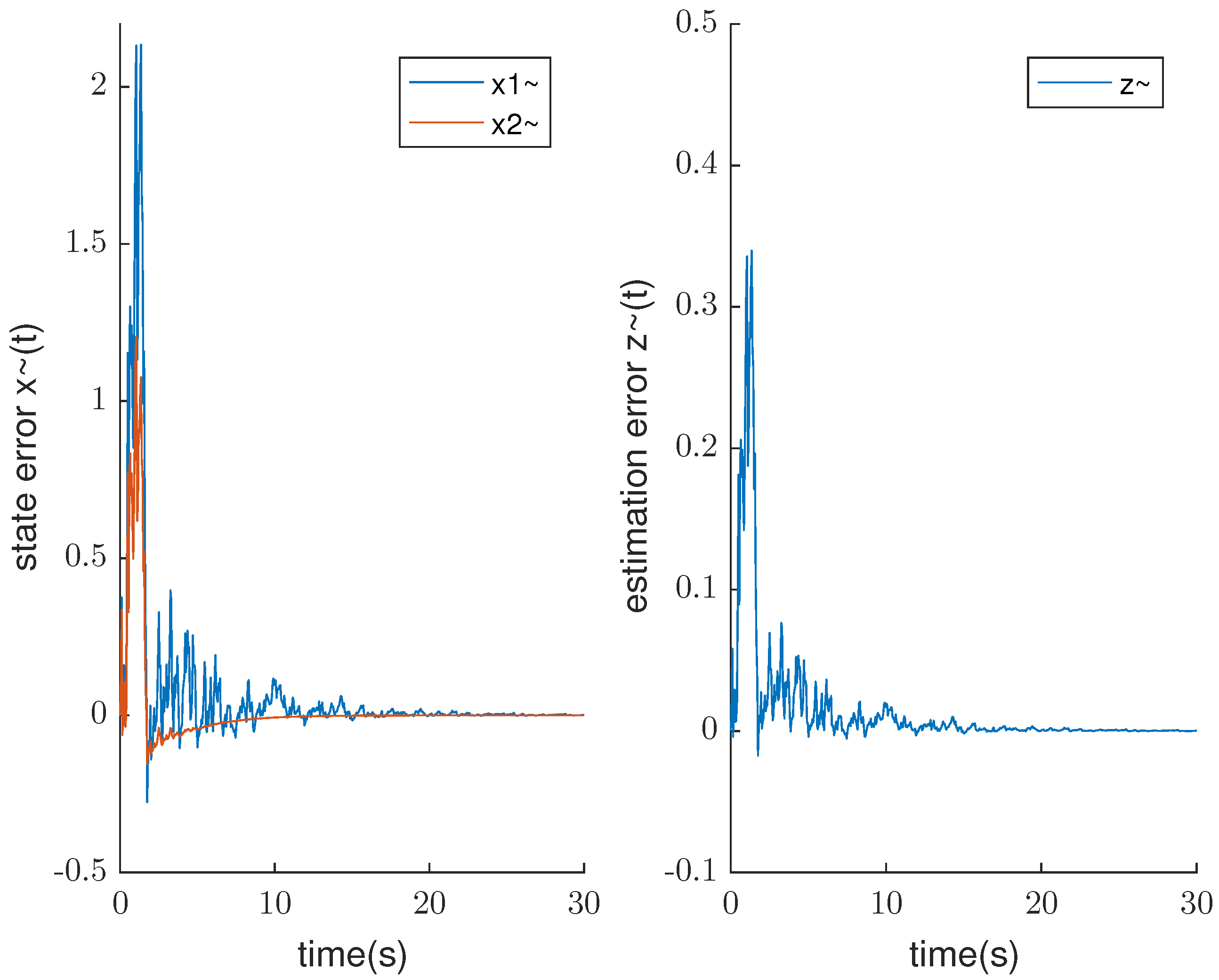
4. Numerical Examples

This section will provide some examples to confirm the validity of the former theoretical analysis.

Example 1.

Consider the mean field stochastic system of one dimension:

$$\left\{\begin{array}{cc}\hfill d{x}_t& =[a{x}_t+\overline{a}E{x}_t+b{v}_t+\overline{b}E{v}_t]dt+[c{x}_t+\overline{c}E{x}_t+d{v}_t+\overline{d}E{v}_t]dw,\hfill \\ \hfill y_t& =k{x}_t+f{v}_t,\hfill \\ \hfill z_t& =l{x}_t+\overline{l}E{x}_t.\hfill \end{array}\right.$$

(17)

In (17), we take

$$\begin{array}{c}\hfill \begin{array}{cc}\hfill a& =-1.7,\overline{a}=-1.3,b=0.7,\overline{b}=0.4,c=0.65,\overline{c}=0.35,\hfill \\ \hfill d& =0.28,\overline{d}=0.12,k=1,f=1.2,l=0.16,\overline{l}=0.1.\hfill \end{array}\end{array}$$

Set $\gamma =1.6$. By solving (9) and (10), we can obtain

$$\begin{array}{c}\hfill \begin{array}{cc}\hfill p_{11}& =0.5,q_{11}=1.2,p_{22}=q_{22}=1.42,z=-0.42,\overline{z}=-0.11,\hfill \\ \hfill z_1& =0.13,{\overline{z}}_1=0.07,l_f=0.09,{\overline{l}}_f=0.06.\hfill \end{array}\end{array}$$

Thus, we have

$$\begin{array}{c}\hfill \begin{array}{cc}\hfill a_f& =p_{22}^{-1}z=-0.2958,{\overline{a}}_f=p_{22}^{-1}\overline{z}=-0.0775,\hfill \\ \hfill b_f& =p_{22}^{-1}{z}_1=0.0915,{\overline{b}}_f=p_{22}^{-1}{\overline{z}}_1=0.0493.\hfill \end{array}\end{array}$$

Accordingly, $H_{\infty }$ filtering can be constructed as

$$\left\{\begin{array}{cc}\hfill d{\widehat{x}}_t& =(-0.2958{\widehat{x}}_t-0.0775E{\widehat{x}}_t)dt+0.0915d{y}_t+0.0493dE{y}_t,\hfill \\ \hfill {\widehat{z}}_t& =0.09{\widehat{x}}_t+0.06E{\widehat{x}}_t.\hfill \end{array}\right.$$

(18)

Denote the error ${\tilde{x}}_t=x_t-{\widehat{x}}_t$. The trajectories of errors ${\tilde{x}}_t$ and ${\tilde{z}}_t$ are plotted in Figure 1.

Example 2.

To help investors avoid possible risks and make more profits by forecasting future stock prices, researchers focuses on the use of mean field stochastic system models to describe real financial systems. For example, in [24], system (1) was used to model the dynamics of stock prices, where $x_t={[x_{1t}^{\top },x_{2t}^{\top }]}^{\top }$ denotes the system state, and $x_{1t}$ and $x_{2t}$ express the stock price of company I and company II, respectively. Specifically, in (1), $E{x}_t$ stands for the impact of the sample moving average. $[C{x}_t+\overline{C}E{x}_t+D{v}_t+\overline{D}E{v}_t]dw$ represents the inherent volatility of stock prices due to random events such as national policies or external circumstances. $v_t$ denotes an exogenous perturbation caused by the general economic environment. $E{v}_t$ indicates the average impact driven by the general economic environment. However, in reality, the presence of $v_t$ results in a system whose states are not fully available and whose statistical properties are not fully known. An estimation of the unavailable state variables can be obtained from the measurement output by means of the design of an $H_{\infty }$ filter.

Let the coefficients of (1) be

$$\begin{array}{c}\hfill \begin{array}{cc}\hfill A& =\left[\begin{array}{cc}-0.9& -0.6\\ 0.7& -1\end{array}\right],\overline{A}=\left[\begin{array}{cc}-0.8& 0.6\\ -0.7& -1\end{array}\right],B=\left[\begin{array}{cc}0.72& -0.2\\ 0.1& 0.8\end{array}\right],\overline{B}=\left[\begin{array}{cc}0.18& 1\\ 1& 0.3\end{array}\right],\hfill \\ \hfill C& =\left[\begin{array}{cc}0.62& -0.2\\ -0.3& 0.61\end{array}\right],\overline{C}=\left[\begin{array}{cc}0.38& -0.2\\ -0.3& 0.39\end{array}\right],D=\left[\begin{array}{cc}0.11& -0.1\\ 0.2& 0.28\end{array}\right],\overline{D}=\left[\begin{array}{cc}0.09& -0.1\\ 0.1& 0.12\end{array}\right],\hfill \\ \hfill K& =\left[\begin{array}{cc}0.1& 0.2\\ 0.3& 0.3\end{array}\right],F=\left[\begin{array}{cc}1& 0.2\\ 0.3& 1\end{array}\right],L=\left[\begin{array}{cc}0.6& 0.3\end{array}\right],\overline{L}=\left[\begin{array}{cc}0.9& 0.4\end{array}\right].\hfill \end{array}\end{array}$$

Choose $\gamma =1.6$. Accordingly, the solutions of (9) and (10) are as follows:

$$\begin{array}{c}\hfill \begin{array}{cc}& P_{11}=\left[\begin{array}{cc}0.5& 0.1\\ 0.1& 0.3\end{array}\right]>0,Q_{11}=\left[\begin{array}{cc}1.3& 0.2\\ 0.2& 1.5\end{array}\right]>0,P_{22}=Q_{22}=\left[\begin{array}{cc}1.4& 0.2\\ 0.2& 1.2\end{array}\right]>0,\hfill \\ & Z=\left[\begin{array}{cc}-8.1& 5.2\\ 4.9& -10.2\end{array}\right],\overline{Z}=\left[\begin{array}{cc}-3.9& 5.8\\ 5.1& -4.8\end{array}\right],Z_1=\left[\begin{array}{cc}0.12& 0.3\\ 0.16& 0.23\end{array}\right],{\overline{Z}}_1=\left[\begin{array}{cc}0.08& 0.2\\ 0.14& 0.17\end{array}\right],\hfill \\ & L_f=\left[\begin{array}{cc}0.16& 0.13\end{array}\right],{\overline{L}}_f=\left[\begin{array}{cc}0.21& 0.11\end{array}\right].\hfill \end{array}\end{array}$$

Therefore, it can be concluded that

$$\begin{array}{c}\hfill \begin{array}{cc}\hfill A_f& =P_{22}^{-1}Z=\left[\begin{array}{cc}-6.5244& 5.0488\\ 5.1707& -9.3415\end{array}\right],{\overline{A}}_f=P_{22}^{-1}\overline{Z}=\left[\begin{array}{cc}-3.4756& 4.8293\\ 4.8293& -4.8049\end{array}\right],\hfill \\ \hfill B_f& =P_{22}^{-1}{Z}_1=\left[\begin{array}{cc}0.0683& 0.1915\\ 0.1220& 0.1598\end{array}\right],{\overline{B}}_f=P_{22}^{-1}{\overline{Z}}_1=\left[\begin{array}{cc}0.0415& 0.1256\\ 0.1098& 0.1207\end{array}\right].\hfill \end{array}\end{array}$$

Consequently, $H_{\infty }$ filtering can be constructed as

$$\begin{array}{cc}\hfill d{\widehat{x}}_t& =\left\{\left[\begin{array}{cc}-6.5244& 5.0488\\ 5.1707& -9.3415\end{array}\right]{\widehat{x}}_t+\left[\begin{array}{cc}-3.4756& 4.8293\\ 4.8293& -4.8049\end{array}\right]E{\widehat{x}}_t\right\}dt\hfill \\ \hfill & +\left[\begin{array}{cc}0.0683& 0.1915\\ 0.1220& 0.1598\end{array}\right]d{y}_t+\left[\begin{array}{cc}0.0415& 0.1256\\ 0.1098& 0.1207\end{array}\right]dE{y}_t,\hfill \\ \hfill {\widehat{z}}_t& =\left[\begin{array}{cc}0.16& 0.13\end{array}\right]{\widehat{x}}_t+\left[\begin{array}{cc}0.21& 0.11\end{array}\right]E{\widehat{x}}_t.\hfill \end{array}$$

The trajectories of the errors ${\tilde{x}}_t$ and ${\tilde{z}}_t$ are plotted in Figure 2.

5. Conclusions

This paper is mainly concerned with the $H_{\infty }$ filtering of mean field stochastic differential systems with state- and disturbance-dependent noise. It is shown that if linear matrix inequalities (9) and (10), which are built upon the mean field stochastic-bounded real lemma, are solvable, then the required $H_{\infty }$ filter can be obtained. Next, we will make future efforts to generalize the proposed results to discrete-time mean field stochastic systems with state-dependent and disturbance-dependent noise.

References

1. McKean, H.P. A class of Markov processes associated with nonlinear parabolic equations. Proc. Natl. Acad. Sci. USA 1996, 56, 1907–1911. [Google Scholar] [CrossRef] [PubMed]
2. Ahdersson, D.; Djehiche, B. A maximum principle for SDEs of mean-field type. Appl. Math. Optim. 2011, 63, 341–356. [Google Scholar] [CrossRef]
3. Li, J. Stochastic maximum principle in the mean-field controls. Automatica 2012, 48, 366–373. [Google Scholar] [CrossRef]
4. Yong, J. A linear-quadratic optimal control problem for mean-field stochastic differential equations. SIAM J. Control. Optim. 2013, 51, 2809–2838. [Google Scholar] [CrossRef]
5. Huang, J.; Li, X.; Yong, J. A linear-quadratic optimal control problem for mean-field stochastic differential equations in infinite horizon. Math. Control. Relat. Fields 2015, 5, 97–139. [Google Scholar] [CrossRef]
6. Ni, Y.; Li, X.; Zhang, J. Mean-field stochastic linear-quadratic optimal control with Markov jump parameters. Syst. Control. Lett. 2016, 93, 69–76. [Google Scholar] [CrossRef]
7. Elliott, R.J.; Li, X.; Ni, Y. Discrete time mean-field stochastic linear-quadratic optimal control problems. Automatica 2013, 49, 3222–3233. [Google Scholar] [CrossRef]
8. Ni, Y.; Elliott, R.J.; Li, X. Discrete time mean-field stochastic linear-quadratic optimal control problems II: Infinite horizon case. Automatica 2015, 57, 65–77. [Google Scholar] [CrossRef]
9. Ahmed, N.U. Nonlinear diffusion governed by McKean-Vlasov equation on Hilbert space and optimal control. SIAM J. Control. Optim. 2007, 46, 356–378. [Google Scholar] [CrossRef]
10. Bjork, T.; Murgoci, A. A general theory of Markovian time incosistent stochastic optimal control problem. SSRN Electron. J. 2010, 18, 545–592, 1694759. [Google Scholar] [CrossRef]
11. Ma, L.; Zhang, W.; Zhao, Y. Study on stability and stabilizability of discrete-time mean-field stochastic systems. J. Frankl. Inst. 2019, 356, 2153–2171. [Google Scholar] [CrossRef]
12. Gao, M.; Zhao, J.; Sun, W. Stochastic H2/H control for discrete-time mean-field systems with Poisson jump. J. Frankl. Inst. 2021, 358, 2933–2947. [Google Scholar] [CrossRef]
13. Wang, M.; Meng, Q.; Shen, Y.; Shi, P. Stochastic H2/H control for mean-field stochastic differential systems with (x,u,v)-dependent noise. J. Optim. Theory Appl. 2023, 197, 1024–1060. [Google Scholar] [CrossRef]
14. Anderson, B.D.O.; Moore, J.B. Optimal Filtering; Prentice-Hall: Englewood Cliffs, NJ, USA, 1979. [Google Scholar]
15. Tseng, C.S.; Chen, B.S. H fuzzy estimation for a class of nonlinear discrete-time dynamic systems. IEEE Trans. Signal Process. 2001, 49, 2605–2619. [Google Scholar] [CrossRef] [PubMed]
16. Gershon, E.; Shaked, U.; Yaesh, I. H control and filtering of discrete-time stochastic systems with multiplicative noise. Automatica 2001, 37, 409–417. [Google Scholar] [CrossRef]
17. Gershon, E.; Limebeer, D.J.N.; Shaked, U.; Yaesh, I. Robust H filtering of stationary continuous-time linear systems with stochastic uncertainties. IEEE Trans. Autom. Control. 2001, 46, 1788–1793. [Google Scholar] [CrossRef]
18. Zhang, W. Robust H filtering of stochastic uncertain systems. Control. Theory Appl. 2003, 20, 741–745. [Google Scholar]
19. Zhang, W. Robust H filtering for nonlinear stochastic systems. IEEE Trans. Signal Process. 2005, 53, 589–598. [Google Scholar] [CrossRef]
20. Yan, S.; Yang, X.; Gu, Z.; Xie, X.; Yang, F. Dynamic sum-based event-triggered H filtering for networked T-S fuzzy wind turbine systems with deception attacks. Fuzzy Sets Syst. 2024, 493, 109084. [Google Scholar] [CrossRef]
21. Zhuang, J.; Li, Y.; Liu, X. Annular finite-time H filtering for mean-field stochastic systems. Circuits Syst. Signal Process. 2024, 43, 2115–2129. [Google Scholar] [CrossRef]
22. Ma, L.; Zhang, T.; Zhang, W.; Pritchard, A.J. H control for continuous-time mean-field stochastic systems. Asian J. Control. 2016, 18, 1–11. [Google Scholar] [CrossRef]
23. Boyd, S.; El Ghaoui, L.; Feron, E.; Balakrishnan, V. Linear Matrix Inequality in Systems and Control Theory; SIAM: Philadelphia, PA, USA, 1994. [Google Scholar]
24. Wu, C.F.; Chen, B.S.; Zhang, W. Multiobjective H2/H control design of the nonlinear mean-field stochastic jump-diffusion systems via fuzzy approach. IEEE Trans. Fuzzy Syst. 2018, 27, 686–700. [Google Scholar] [CrossRef]
Figure 1. The trajectories of the errors x ˜ t and z ˜ t .
Mathematics 12 03329 g001
Figure 2. The trajectories of errors x ˜ t and z ˜ t .
Mathematics 12 03329 g002
Disclaimer/Publisher’s Note: The statements, opinions and data contained in all publications are solely those of the individual author(s) and contributor(s) and not of MDPI and/or the editor(s). MDPI and/or the editor(s) disclaim responsibility for any injury to people or property resulting from any ideas, methods, instructions or products referred to in the content.