Abstract
This paper elucidates the prerequisites for maximum likelihood estimation (MLE) of parameters within the exponential and scale parameter families. Estimation of these parameters is predicated on data derived from censored samples and seeks to adhere to stochastic ordering principles. The study establishes that for two independent normal distributions and a two-parameter exponential distribution discernible by the distinct parameter sets, the MLEs of the parameters evince a stochastically ordered relationship when evaluated using full datasets. Furthermore, this research is extended to corroborate the persistence of stochastic ordering in the MLEs of such parameters under conditions of fixed censoring of samples.
Keywords:
usual random order; censored samples; maximum likelihood estimator; location family; scale family MSC:
90B25; 60E05
1. Introduction
In medical research, finance, service industries, and business analytics, the exponential distribution and MLE are pivotal. Among other things, they assess treatment outcomes amid censored survival data, gauge risks for insurance purposes, optimize service delivery in call centers, ensure stochastic order for decision-making, facilitate statistical inferences from incomplete datasets, and validate model accuracy. This approach is paramount for efficient resource management and informed strategic planning across sectors.
In a series of examples, such as life-test or reliability tests, there is prior information available about the parameters. An experimenter can use this prior information to judge that a product is more reliable than its competitive product. In this scenario, the expectation is that parameter estimation will also effectively capture the comparative magnitudes of the parameters. Numerous inferential methods for estimating global parameters under these ordered constraints have been explored. The literature provides comprehensive details on inferential techniques for order constraints, as presented by Barlow (1972) [1] and expanded upon by Nuesch (1999) [2], among others.
N. Balakrishnan and Jiemi (2001) [3] proposed the random order problem for maximum likelihood estimation of parameters under the full sample, and proposed three conditions for single parameter distribution based on the maximum likelihood estimate of the full sample. The random order theory is a set of theories about the “size” of random variables. In a certain sense, it can be used to compare one random variable (vector) in terms of its size or number of variables with respect to another random variable (vector) [4,5,6]. Random order is a theoretical tool and method for decision-making in random environments, and is also a typical representative of uncertain variable comparison [7,8,9,10]. The study of random order has a wide and profound practical background, making it of great significance in both theory and application [11,12,13,14,15].
The life test is divided into the complete life test and the censored life test according to the failure of the sample, with the latter being the most widely used. Bartholomew (1957) [16] mentioned some problems and solutions that may arise during life test. The exponential distribution is one of the more widely used distributions for modeling life in reliability theory and practical reliability engineering [17,18,19]. Many useful results on exponential distributions can be found in [20,21]. The problem of estimating the mean of the exponential distribution is very important, and different maximum likelihood estimates can exist depending on the censored sample.
Consider a population that has a probability density function , where the parameter belongs to a subset of . One important aspect of statistical inference is obtaining a point estimator of . Many different methods of estimation are known in the literature, for example moment estimation, maximum likelihood estimation, least-squares estimation, etc. [22]. Various properties of these approaches, such as unbiasedness, weak and strong consistency, and asymptotic normality, have been discussed; in this paper, our aim is as follows: based on censored samples, we discuss the conditions under which the maximum likelihood estimates of the parameters of the family of exponential distributions satisfy random ordering [23,24,25,26].
By “order preserving”, we refer to the following concept: suppose that X and Y are independent of each other from two exponentially distributed aggregates, with , , …, a sample from the aggregate and , , …, a sample from population . Assume that , , and further that . We denote the point estimators of and obtained from applying the same estimation method based on and by and , respectively. Let , , …, and , , …, be Type-I censored samples, where , . Because the real parameter values and satisfy , it is desirable that a certain order exist between their point estimators and . In general, it cannot be true that point-wise due to the randomness of samples. Then, it is of interest to investigate what kind of order may exist between and . Because of its popularity and importance, a natural candidate for possible order between and is the usual stochastic order ≤.
Definition 1.
If the random variables X and Y have distribution functions and , we say that X is stochastically less than or equal to Y if , , which is denoted by or .
In comparison to the various stochastic orders known in the literature, the order ≤ or ≥ is not a restrictive one; however, even this order does not always hold between and , as the following example indicates.
Studying the order preservation of maximum likelihood estimates obtained from censored samples can verify consistency, rank parameters, perform variable selection, and evaluate robustness, helping us to better understand and apply maximum likelihood estimation methods. Consistency means that the maximum likelihood estimates converge to the true parameters as the sample size approaches infinity. By studying the order preservation of maximum likelihood estimates under truncated samples, we can further verify the consistency of maximum likelihood estimates in finite samples. Order preservation studies allow for parameter ranking. Through the analysis of order preservation after removing samples, we can compare the order of parameter estimates under different models or hypotheses, identify important parameters or model features, and help to understand the influence and importance of parameters. In regression models with a large number of predictors, analyzing the order preservation of parameter estimates after sample removal can help in selecting important variables based on the order preservation of parameter estimates, which not only reduces model complexity but also enhances model interpretability and prediction accuracy. In the presence of outliers or extreme observations, analyzing the order preservation after removing samples can quantify the sensitivity of maximum likelihood estimates to outliers and help to evaluate the robustness and stability of parameter estimates.
The rest of the paper is organized as follows. We demonstrate in Section 2 that the maximum likelihood estimators (MLEs) of the single-parameter exponential distribution, double-parameter exponential distribution, and normal distribution, which are part of the exponential family, exhibit stochastic order relations under complete sampling. In Section 3, we present the general form of the exponential family distribution and the specific conditions required for the location and scale parameter families to satisfy stochastic order in censored samples, followed by a numerical analysis. Section 4 details the conditions under which the MLEs of the double-parameter exponential distribution meet the criteria for stochastic order in the context of censored samples. Section 5 provided illustrative examples to clarify these concepts.
2. Comparison of MLE under Complete Samples
2.1. One-Parameter Exponential Distribution
Let be an integrable function on for each and let be defined by
In addition, we denote
Here, is a valid probability density function on . Suppose that and that the random variables X and Y have density functions and , respectively. Furthermore, let and , be censored samples under and , respectively. The following result provides the conditions under which , and the maximum likelihood estimators and for and satisfy . Throughout this article, it is always assumed that the maximum likelihood estimator belonging to the parameter space exists and is unique. The conditions that guarantee this are not provided explicitly.
Lemma 1.
Let be defined by (1) and (2).
Suppose that:
- 1.
- is log-concave, i.e., ,;
- 2.
- is log-concave in , i.e., , , ;
- 3.
- , ,.
If and at least one of the inequalities in 1–3 is strict, then there is and .
The above lemma provides a general condition for the MLE to have the property of preserving the usual stochastic orders. It is given that when conditions 1, 2, and 3 are satisfied, two mutually independent exponentially distributed random variables exist under the equivalent carve-outs under the usual random order.
2.2. Two-Parameter Exponential Distribution
Theorem 1.
Let the samples follow a two-parameter exponential distribution with probability density function
and let the samples follow a two-parameter exponential distribution with probability density function
If
then the maximum likelihood estimators and obtained from satisfy the stochastic order relationship with the maximum likelihood estimators and obtained from , denoted as
Proof.
The likelihood function of is
and its log-likelihood function is
Observing the expression of , for any fixed , in order to maximize the likelihood function must be as large as possible with . The likelihood function reaches its maximum; hence, ,and then , where . Thus, we have
Knowing , we aim to find , that is, ,
From
we know that the above formula holds, that is, .
Given that , we want to obtain , that is,
Because
and , we have
therefore, . This completes the proof of Theorem 1. □
2.3. Normal Distribution
Theorem 2.
Let the samples follow a normal distribution with probability density function
and let the samples follow a normal distribution with probability density function
If and , then the maximum likelihood estimators and obtained from satisfy the stochastic order relationship with the maximum likelihood estimators and obtained from , which we denote as and .
Proof.
For all t, the probability if and only if
where the random variable follows a standard normal distribution . Therefore,
Given that and , it follows that
which implies
indicating that .
To achieve , it suffices to show that for all t, . To this end, we can consider
Because , it follows that follows a chi-squared distribution with n degrees of freedom. Therefore,
Given that , it follows that ; thus,
which implies
confirming that . □
3. Comparison of MLEs under Censored Samples
3.1. Generalization of the Exponential Distribution
Theorem 3.
Assuming that the exponential distributions of populations X and Y are independent, the parameters are and , respectively. Suppose that ,,…, are lifetimes following the exponential distribution with parameter , while ,,…, are lifetimes following the exponential distribution with parameter . Given , let be the number of that satisfies and be the number of that satisfies ,,. Moreover, and are maximum likelihood estimators of and . Suppose that:
- (I)
- increases with respect to θ, while and its derivatives are continuous and decreases with respect to θ;
- (II)
- ,, , ;
If , then there is (a) and (b) .
Proof.
We shall first prove (a). For any , we have
Note that condition (I) implies that
which is equivalent to
From (1) and (2), we can see that increases in . This means that X is smaller than Y in the likelihood ratio order denoted by . This order further yields ; hence, (a) is proved.
Because and are censored samples, they are independent and identically distributed; in addition, is known from conclusion (a), and there is a random variable known by the coupling method that makes point by point, where and have the same distribution.
If n products are put into the timing truncation experiment, the truncation time is t and the timing truncation sample is obtained, that is, r products fail in the time interval and do not fail at time . The probability of a product failure in the interval is approximately , . The probability of the remaining product life exceeding is .
Therefore, the likelihood function of the sample is
i.e.,
Thus, we can know that is determined by
while is determined by
To prove , it is sufficient to show that is pointwise, that is,
Using the coupling method, we obtain .
Now, we shall prove that pointwise. Let us first assume the contrary, that is, that holds on a set of positive probabilities. From condition 1, the function decreases in ; hence, it follows that on the set we have
Inequalities (19), (21), and (23) imply that
From condition (I), it can be seen that
and consequently that
Because pointwise , from (25) it follows that
On the other hand, it is true that
Because Lemma 1 implies that decreases in for any and , by combining (26) and (27) we obtain
and consequently,
Because of , we have
According to condition (I),
is increased with respect to and ; thus, we have
Also from condition (I),
decreases with respect to and ; thus, we have
From Condition (II), ; thus, it is apparent that
Because at least one of conditions (I) or (II) is strictly established, we can combine (29) and (30) to obtain
This contradicts (24), meaning that the hypothesis does not hold; thus, is further obtained by , and is proved. □
Example 1.
For the gamma density function , where is known, it can be verified that conditions (I) and (II) in Theorem 1 are satisfied. Let ; then,
Therefore, the conditions in Theorem 3 are all satisfied, and if , then there is .
Example 2
(Beta Distribution). Consider the beta density function
with known . This is an exponential family density with . It can be verified that all the conditions of Theorem 3 are satisfied. In particular, we have
Hence, implies that . Similarly, assuming that α is known, it can be shown that implies the maximum likelihood estimators .
3.2. Location and Scale Family
It can be seen that Theorem 1 cannot be applied to the exponential density function .
To better study the randomness of the maximum likelihood estimator under censored samples, Theorem 3 needs to be further improved.
Assuming that is a probability density function defined on the interval , then for any , the density function set
is called the scale distribution family.
Theorem 4.
Let :
- (i)
- is strictly increasing with respect to ;
- (ii)
- ,, , ;
If , then (a) ; further, if is either strictly log-concave or strictly log-convex, then (b) .
Proof.
We shall first prove (a).
Let be an independent and identically distributed random variable with the common probability density . Furthermore, let be an independent and identically distributed random variable with common probability density .
Using the coupling method, it can be seen that there is an independent and identically distributed random variable such that pointwise; moreover, has the same distribution as . Then, and can be proved as in Theorem 1, providing .
Without loss of generality, we simply assume that pointwise; thus, we need to show that pointwise.
Using the contradiction method, suppose that ; then, in the set , we have .
From (32), under the condition of censored samples (assuming the censored number is r), is determined by
and is determined by
that is, it always holds that
Because is strictly increasing and , we have
and ; thus,
From the condition
we can obtain
Inequalities (37) and (38) imply that
As (35) and (39) are contradictory, the hypothesis does not hold; therefore, is proved. □
Example 3.
Consider the function
with known and satisfying the conditions in Theorem 4. Therefore, if , then there is , In particular, when , it is an exponential distribution, which is also true.
Example 4.
The logistic distribution with density
satisfies the conditions of Theorem 4; thus, if , then .
Now, let us investigate the scale family. Suppose that is a probability density function on . For any , forms a density on . We refer to the collection of density functions as a scale family of distribution.
The scale parameter can be reduced to a location parameter by logarithmic transform. Therefore, the following result follows immediately from Theorem 4.
3.3. Numerical Examples
As part of this study, we conducted a simulation analysis on two exponential populations with parameters and . We employed censored data with a predetermined number of failures to obtain the maximum likelihood estimator . For each of these two exponential distributions, 50 experimental units were tested and the required sample data were recorded to apply this method. This experiment was repeated 1000 times. Based on the 1000 values of corresponding to each population under this method, the empirical cumulative distribution functions (ECDFs) of were calculated.
The empirical cumulative distribution functions (ECDFs) of associated with and obtained by applying censoring with are plotted in Figure 1.
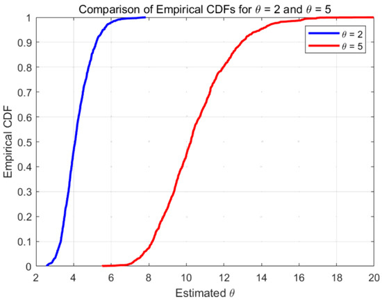
Figure 1.
Censoring with .
3.4. Data Analysis
We used numerical simulation to analyze a practical application as a case study. The Monte Carlo method was used to randomly generate samples from the exponential distributions of and with sample sizes of 10, 50, 100, 200, and 500. The maximum likelihood estimates of parameters and , denoted as and , were obtained from each set of simulated data. The entire program was repeated 5000 times, with the bias and mean square error (MSE) used to evaluate the maximum likelihood estimates. The calculation formulas are as follows:
and
Table 1 shows the maximum likelihood estimates, biases, and mean square errors for parameters and of the exponential distribution. It can be observed that the maximum likelihood estimates for both parameters approach the true values as the sample size increases. Furthermore, the biases and mean square errors decrease as the sample size increases, indicating that the maximum likelihood estimation exhibits good stability.

Table 1.
Monte Carlo simulation results of the exponential distribution.
4. Two-Parameter Exponential Distribution
Theorem 5.
In addition, we performed a tailing experiment on two sets of samples with a capacity of n. Here, the tail number is m, the tailed samples obey the two-parameter exponential distribution
and the tailed samples obey the two-parameter exponential distribution
If
then there is
where are the censored maximum likelihood estimators obtained from and are the censored maximum likelihood estimators obtained from .
Proof.
The likelihood function of is as follows:
and its log-likelihood function is
In order to make the likelihood function reach the maximum value, we have according to the context, and
Similarly,
Because
are given, we can use a proof method similar to that in Theorem 4 to obtain
□
5. Illustrative Example
Assume that we have two types of batteries and that their lifetimes follow exponential distributions with parameters (i.e., the average lifetime is 100 h) and (i.e., the average lifetime is 120 h). We want to test the stochastic order of the lifetimes of the two types of batteries.
We can draw 50 samples from each distribution, but only record the lifetime data exceeding 80 h (censoring point h).
The following are the sample data (in hours) drawn from the two distributions, listing only the samples exceeding 80 h:
Battery Type 1:
- Samples: 82, 85, 90, 84, 81, 83, 85, 89, 88, 87, …
Battery Type 2:
- Samples: 81, 86, 92, 83, 85, 87, 90, 82, 84, 88, ….
For the exponential distribution, the MLE can be calculated using the following formula:
where n is the sample size and are the sample data.
Assuming the calculations yield
we then need to verify whether holds. Because , it is implied that , meaning that Battery Type 1 has a higher failure rate. As we are interested in the lifespan, we can conclude that Battery Type 2 has a longer lifespan.
Based on the maximum likelihood estimates, we can conclude that Battery Type 2 has a longer lifespan, satisfying the condition of stochastic order .
This practical example demonstrates how to compare the lifespan distributions of batteries with different parameters using the MLEs from censored samples and infer differences in battery performance through stochastic order.
6. Conclusions
In this study, we have successfully validated two crucial theorems which establish that maximum likelihood estimators (MLEs) for parameters associated with location and exponential distribution families maintain stochastic ordering when estimated from censored samples provided that certain conditions are met. Furthermore, we provide practical examples that demonstrate the applicability of these theorems in real-world scenarios.
Author Contributions
Conceptualization, Y.L.; methodology, J.R., X.L. and P.L.; software (R language 4.3): J.R.; formal analysis, C.G.; data curation, P.L.; writing—original draft, J.R. and X.L.; writing—editing, C.G. and J.R.; project administration, Y.L., C.G. and J.R.; funding acquisition, J.R. All authors have read and agreed to the published version of the manuscript.
Funding
This paper was supported by the Shanghai University of Finance and Economics, Zhejiang College Educational Committee (Grant No. 2020 GR007).
Data Availability Statement
The data that support the findings of this study are available from the corresponding author upon reasonable request.
Conflicts of Interest
The authors declare no conflicts of interest.
References
- Brunk, H.D.; Barlow, R.E.; Bartholomew, D.J.; Bremner, J.M. International Statistical Review. In Statistical Inference under Order Restrictions; Wiley: Hoboken, NJ, USA, 1972; Volume 41, pp. 395–412. [Google Scholar]
- Nuesch, P.E. Order Restricted Statistical Inference. J. Appl. Econom. 1991, 6, 105–107. [Google Scholar]
- Viveros, R.; Balakrishnan, N. Interval estimation of parameters of life from progressively censored data. Technometrics 1994, 36, 84–91. [Google Scholar] [CrossRef]
- Balakrishnan, N.; Brain, C.; Mi, J. Stochastic order and MLE of the mean of the exponential distribution. Methodol. Comput. Appl. Probab. 2001, 4, 83–93. [Google Scholar] [CrossRef]
- Balakrishnan, N.; Mi, J. Order-preserving property of maximum likelihood estimator. J. Stat. Plan. Inference 2001, 98, 89–99. [Google Scholar] [CrossRef]
- Bain, L.J.; Engelhardt, M. Interval estimation for the two-parameter double exponential distribution. Technometrics 1973, 15, 875–887. [Google Scholar] [CrossRef]
- Kng, F.; Fei, H. Limit theorems for the maximum likelihood estimate under general multiply Type II censoring. Ann. Inst. Stat. Math. 1996, 48, 731–755. [Google Scholar]
- Cohen, C.A.; Whitten, B. Modified maximum likelihood and modified moment estimators for the three-parameter Weibull distribution. Commun. Stat.-Theory Methods 1982, 11, 2631–2656. [Google Scholar] [CrossRef]
- Prajapati, D.; Mitra, S.; Kundu, D. A new decision theoretic sampling plan for type-I and type-I hybrid censored samples from the exponential distribution. Sankhya B 2019, 81, 251–288. [Google Scholar] [CrossRef]
- Krishnamoorthy, K.; Xia, Y. Confidence intervals for a two-parameter exponential distribution: One-and two-sample problems. Commun. Stat.-Theory Methods. 2018, 47, 935–952. [Google Scholar] [CrossRef]
- Rényi, A. On the theory of order statistics. Acta Math. Acad. Sci. Hung. 1953, 4, 48–89. [Google Scholar] [CrossRef]
- Kundu, D.; Kannan, N.; Balakrishnan, N. Analysis of progressively censored competing risks data. Handb. Stat. 2003, 23, 331–348. [Google Scholar]
- Guo, M.-Y.; Zhang, J.; Yan, R. Stochastic comparisons of second largest order statistics with dependent heterogeneous random variables. Commun. Stat.-Theory Methods 2024, 1–19. [Google Scholar] [CrossRef]
- Qiu, G.; Raqab, M. On weighted extropy of ranked set sampling and its comparison with simple random sampling counterpart. Commun. Stat.-Theory Methods 2024, 53, 378–395. [Google Scholar] [CrossRef]
- Crescenzo, A.D.; Paolillo, L.; Suárez-Llorens, A. Stochastic comparisons, differential entropy and varentropy for distributions induced by probability density functions. Metrika 2024, 1–17. [Google Scholar] [CrossRef]
- Bartholomew, D.J. A problem in life testing. J. Am. Stat. Assoc. 1957, 52, 350–355. [Google Scholar] [CrossRef]
- Al-Athari, M.F.M. Estimation of the mean of truncated exponential distribution. J. Math. Stat. 2008, 4, 284. [Google Scholar] [CrossRef]
- Weißbach, R.; Wied, D. Truncating the exponential with a uniform distribution. Stat. Pap. 2022, 63, 1247–1270. [Google Scholar] [CrossRef]
- Hannon, P.M.; Dahiya, R.C. Estimation of parameters for the truncated exponential distribution. Commun. Stat.-Theory Methods. 1999, 28, 2591–2612. [Google Scholar] [CrossRef]
- Hu, Y.-H.; Emura, T. Maximum likelihood estimation for a special exponential family under random double-truncation. Comput. Stat. 2015, 30, 1199–1229. [Google Scholar] [CrossRef]
- Sabti, A.N.; Ansseif, A.A.l.; Shakir, A.M. Estimating the Reliability for the Sequential System of Two Truncated Exponential Distribution. Ind. Eng. Manag. Syst. 2021, 20, 455–463. [Google Scholar] [CrossRef]
- Raschke, M. Inference for the truncated exponential distribution. Stoch. Environ. Res. Risk Assess. 2012, 26, 127–138. [Google Scholar] [CrossRef]
- Blumenthal, S.; Dahiya, R.C. Estimating scale and truncation parameters for the truncated exponential distribution with type-I censored sampling. Commun. Stat.-Theory Methods 2005, 34, 1–21. [Google Scholar] [CrossRef]
- Suich, R.; Rutemiller, H.C. Point Estimation of the Parameter of a Truncated Exponential Distribution. IEEE Trans. Reliab. 1982, 31, 393–397. [Google Scholar] [CrossRef]
- Akahira, M. Statistical Estimation for Truncated Exponential Families; Springer: Berlin/Heidelberg, Germany, 2017. [Google Scholar]
- Kumar, D.; Dey, S.; Nadarajah, S. Extended exponential distribution based on order statistics. Commun. Stat.-Theory Methods 2017, 46, 9166–9184. [Google Scholar] [CrossRef]
Disclaimer/Publisher’s Note: The statements, opinions and data contained in all publications are solely those of the individual author(s) and contributor(s) and not of MDPI and/or the editor(s). MDPI and/or the editor(s) disclaim responsibility for any injury to people or property resulting from any ideas, methods, instructions or products referred to in the content. |
© 2024 by the authors. Licensee MDPI, Basel, Switzerland. This article is an open access article distributed under the terms and conditions of the Creative Commons Attribution (CC BY) license (https://creativecommons.org/licenses/by/4.0/).