Application of Kirchhoff Migration from Two-Dimensional Fresnel Dataset by Converting Unavailable Data into a Constant

Abstract

In this contribution, we consider an application of the Kirchhoff migration (KM) technique for fast and accurate identification of small dielectric objects from two-dimensional Fresnel experimental dataset. Generally, for successful application of the KM, a complete set of elements from the so-called multi-static response (MSR) matrix must be collected; however, in the Fresnel experimental dataset, many of the elements of an MSR matrix are not measurable. Nevertheless, the existence, location, and outline shape of small objects can be retrieved using the KM by converting unavailable data into the zero constant. However, the theoretical reason behind such conversion has not been confirmed to date. In order to explain this theoretical reason, we convert unavailable measurement data into a constant and demonstrate that the imaging function of the KM can be expressed by an infinite series of the Bessel functions of integer order of the first kind, the object’s material properties, and the converted constant. Following the theoretical result, we confirm that converting unknown data into the zero constant guarantees good results and unique determination of the objects. Finally, various numerical simulation results from Fresnel experimental dataset are presented and discussed to validate the theoretical result.

1. Introduction

Inverse scattering problems, which deal with the reconstruction of the existence, location, and shape of small objects without a priori information, are an interesting and important research subject in applied mathematics, physics, engineering, and medical sciences. Various reconstruction techniques have been investigated to solve inverse scattering problems, and these can be classified as iterative and non-iterative approaches.

Generally, iterative (or quantitative) techniques are employed to reconstruct the distribution of parameters, e.g., the relative permittivity, magnetic permeability, and electrical conductivity in a region, and various important and interesting techniques have been investigated, e.g., the Gauss–Newton method for biomedical imaging [1], crack detection in nondestructive testing [2], the Newton–Kantorovich method for arm imaging [3], the Levenberg–Marquardt algorithm for anomaly detection [4], the Nelder–Mead simplex method to search buried object [5], the level-set technique to retrieve arbitrary shaped scatterers [6], the potential drop method to evaluate crack depth [7], topological derivative for shape optimization [8], and the Newton method for crack reconstruction [9]. Iterative techniques have been applied successfully across various fields; however, several important issues must be addressed prior to their implementation. These issues include obtaining a priori information about the unknown targets, evaluating the complex Fréchet derivative at each iteration step, selecting an appropriate regularization, and generating an initial guess that is sufficiently close to the unknown target. Without a good initial guess, the iterative procedures may face critical issues, e.g., non-convergence, falling into local minima, and incurring substantial computational costs, refer to [10,11]. Thus, it is natural to consider the generation of a good initial guess without a priori information of the unknown objects.

Alternatively, various non-iterative (or qualitative) techniques have been investigated to identify the existence, location, and shape of objects, and such methods have been applied to various inverse scattering problems and microwave imaging, e.g., the bifocusing method for damage detection of concrete voids [12] and tomographic radar imaging [13], direct sampling methods to identify small targets [14] and detect anomalies [15], factorization method for crack detection [16] in inverse scattering problem and breast cancer detection in microwave imaging [17], the MUltiple SIgnal Classification (MUSIC) algorithm for virtual electrical breast biopsy [18] and anomaly imaging in real-world microwave imaging [19], the linear sampling method for underwater acoustic imaging [20] and the limited-aperture inverse scattering problem [21], subspace migration for objects localization in limited-aperture inverse scattering problem [22] and microwave imaging [23], and the topological derivative strategy for fast imaging of crack-like defects [24] and flaw detection in welding joints [25].

Kirchhoff migration (KM) is a powerful non-iterative method to identify arbitrary shaped objects. The KM has been used in a wide range of studies, e.g., imaging volcanic fields [26], identifying arbitrary objects embedded in a random medium [27], inversion of phaseless data [28], terahertz imaging [29], anomaly imaging in microwave imaging [30], real-time tracking of moving objects [31], and radar imaging [32]. Note that the KM is a very effective, robust, stable technique for both inverse scattering problems and microwave imaging; however, for successful application of the KM, all elements of the so-called multi-static response (MSR) or scattering matrices must be available.

Unfortunately, in many real-world applications, many elements of such matrices are not available due to limitations in data acquisition processes. For example, in microwave imaging [33], the diagonal elements of the matrix cannot be handled because each antenna is used for signal transmission, and the remaining antennas are used for signal reception. Recently, it has been confirmed theoretically that the existence and location of small dielectric objects can be identified uniquely using the KM by converting unavailable data into a zero constant [31]. With another inverse problem using an experimental Fresnel dataset [34], many elements of the matrix, including the diagonal elements, cannot be measured because a receiver is rotating with a limited range based on each direction of the transmitters when a transmitter is placed at a fixed position. Similar to the traditional approach, by converting the unknown measurement data into the zero constant, it is possible to identify the existence and outline shape of small objects using the KM.

Otherwise, converting unavailable data into a nonzero constant does not guarantee good results. Generally, the imaging results obtained using the KM are very poor when the absolute value of the converted constant is not sufficiently small. However, to the best of our knowledge, there is no theoretical result for the influence of the converted constant. To address this issue, this study explores the structure of the imaging function of the KM from the 2D Fresnel dataset by converting unmeasurable data into a fixed constant. Based on the fact that the measured scattering field can be expressed in the form of an integral equation, we demonstrate that the imaging function can be expressed by an infinite series of Bessel functions of integer order of the first kind and converted constant. Based on the theoretical result, it is possible to explain that the imaging performance is strongly dependent on the converted constant and that the conversion of the zero constant guarantees good imaging results, including the unique determination of objects. Various simulation results obtained on the 2D Fresnel dataset are presented to validate the theoretical result.

The remainder of this paper is organized as follows. Section 2 briefly introduces the two-dimensional direct scattering problem in the presence of small dielectric objects and the imaging function of the KM by converting the unavailable elements of the MSR matrix into a fixed constant. In Section 3, we demonstrate that the imaging function comprises an infinite series of Bessel functions of integer order of the first kind and converted constants, and in Section 4, we discuss various intrinsic properties of the imaging function and conclude that converting the zero constant guarantees good imaging results. To support the theoretical result, Section 5 presents simulation results obtained at various frequencies using the 2D Fresnel experimental dataset. Finally, a brief conclusion, including a future research topic, is provided in Section 6.

2. Two-Dimensional Simulation Configuration and Kirchhoff Migration

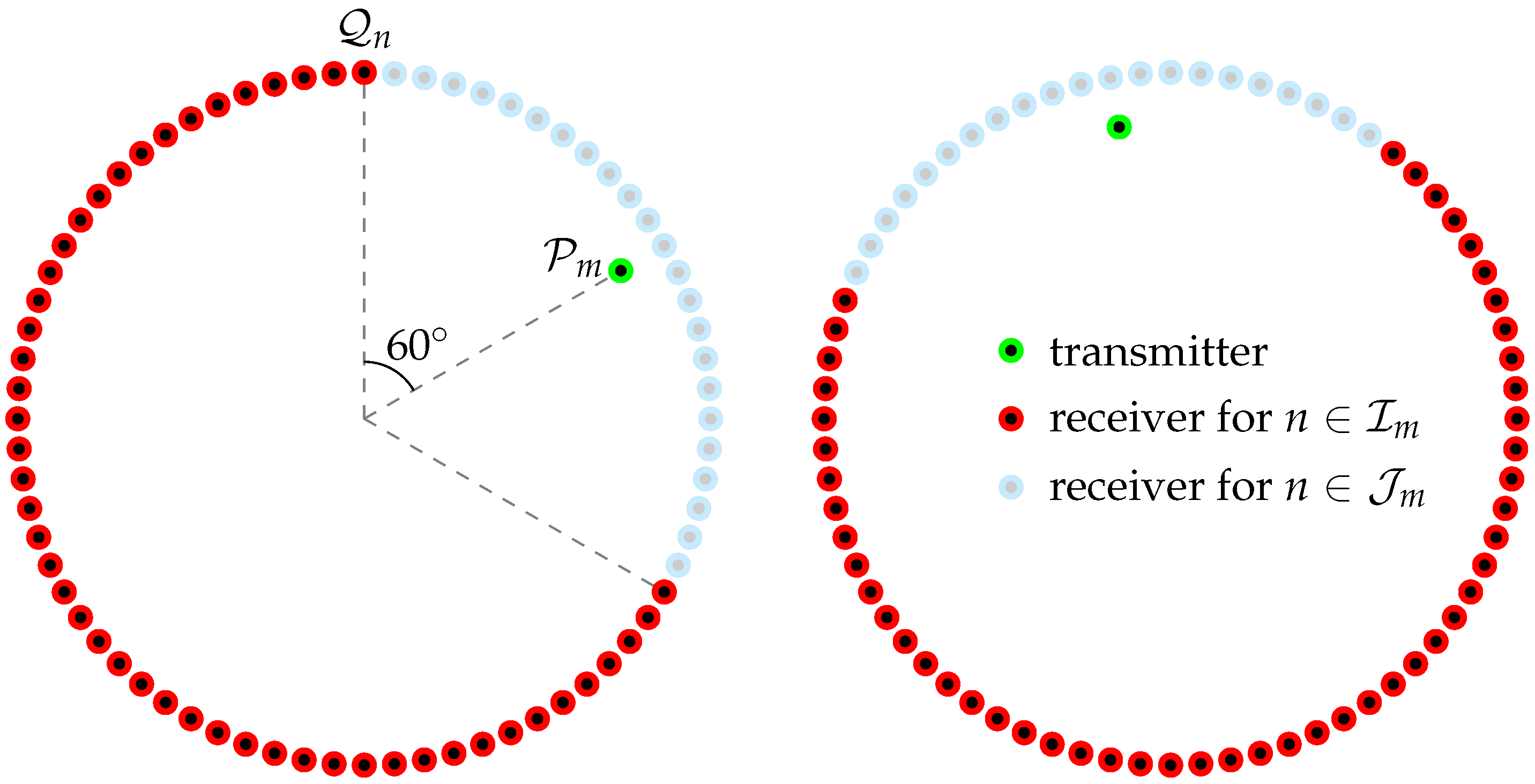
2.1. Problem Configuration and Representation Formula for the Scattered Field

In the following, we describe the simulation configuration introduced in the literature [34]. Here, ${\mathcal{P}}_m$, $m=1,2,\dots ,M$, and ${\mathcal{Q}}_n$, $n=1,2,\dots ,N$ represent the mth transmitter and nth receiver with locations ${\mathbf{p}}_m$ and ${\mathbf{q}}_n$, respectively, such that

$$\begin{array}{cc}\hfill {\mathbf{p}}_m& =P{\mathsf{\vartheta }}_m=0.72\mathrm{m}(cos{\vartheta }_m,sin{\vartheta }_m)\hfill \\ \hfill {\mathbf{q}}_n& =Q{\mathsf{\theta }}_n=0.76\mathrm{m}(cos{\theta }_n,sin{\theta }_n),\hfill \end{array}$$

where ${\vartheta }_m=(m-1)▵\vartheta =(m-1){10}^{\circ }$ and ${\theta }_n=(n-1)▵\theta =(n-1)5^{\circ }$. Here, the total number of transmitters and receivers is $M=36$ and $N=72$, respectively. In addition, $\mathcal{P}$ and $\mathcal{Q}$ denote the collection of transmitters ${\mathcal{P}}_m$ and receivers ${\mathcal{Q}}_n$, respectively.

Let $\Omega$ be a two-dimensional homogeneous region, and the transmitters ${\mathcal{P}}_m$ and receivers ${\mathcal{Q}}_n$ are located at the exterior of $\Omega$. Assume that there exist well-separated small objects $D_s\subset \Omega$, $s=1,2,\dots ,S$ with smooth boundaries, and all objects are completely characterized by their dielectric permittivity value at a given angular frequency $\omega =2\pi f$. Throughout, D denotes the collection of $D_s$, and ${\epsilon }_s$ and ${\epsilon }_{\mathrm{b}}$ denote the permittivity value of $D_s$ and $\Omega$, respectively, and we assume that ${\epsilon }_s>{\epsilon }_{\mathrm{b}}$ for all $s=1,2,\dots ,S$. Following the literature [34], $\Omega$ can be considered a vacuum; thus, for each $\mathbf{x}\in \Omega$, the background conductivity, permeability, and permittivity values are set to $\sigma \left(\mathbf{x}\right)\equiv {\sigma }_{\mathrm{b}}\approx 0\mathrm{S}/\mathrm{m}$, $\mu \left(\mathbf{x}\right)\equiv {\mu }_{\mathrm{b}}=4\pi \times {10}^{-7} \mathrm{H}/\mathrm{m}$ and ${\epsilon }_{\mathrm{b}}={\epsilon }_0=8.854\times {10}^{-12} \mathrm{F}/\mathrm{m}$, respectively. Based on this, $k=\omega \sqrt{{\epsilon }_0{\mu }_0}$ denotes the background wavenumber, and we introduce the following piecewise constant of permittivity:

$$\epsilon \left(\mathbf{x}\right)=\left\{\begin{array}{ccc}{\epsilon }_s& \mathrm{if}& \mathbf{x}\in D_s\hfill \\ {\epsilon }_{\mathrm{b}}& \mathrm{if}& \mathbf{x}\in \Omega \setminus \overline{D}.\hfill \end{array}\right.$$

Let $u_{inc}(\mathbf{x},{\mathbf{p}}_m)$ be the incident field generated at the mth transmitter:

$$u_{inc}(\mathbf{x},{\mathbf{p}}_m)=G(\mathbf{x},{\mathbf{p}}_m)=-{\displaystyle \frac{i}{4}}{H}_0^{\left(1\right)}\left(k\right|\mathbf{x}-{\mathbf{p}}_m\left|\right),$$

where $H_0^{\left(1\right)}$ denotes the zero order Hankel function of the first kind. We denote $u(\mathbf{x},{\mathbf{p}}_m)$ as the time-harmonic total field that satisfies the following scalar Helmholtz equation:

$$▵u(\mathbf{x},{\mathbf{p}}_m)+{\omega }^2\epsilon \left(\mathbf{x}\right){\mu }_{\mathrm{b}}u(\mathbf{x},{\mathbf{p}}_m)=0,\mathbf{x}\in \Omega$$

with transmission condition at $\partial D_s$. Throughout this paper, $u_{scat}({\mathbf{q}}_n,{\mathbf{p}}_m)=u({\mathbf{q}}_n,{\mathbf{p}}_m)-u_{inc}({\mathbf{q}}_n,{\mathbf{p}}_m)$ denotes the scattered field measured at the nth receiver that satisfies the Sommerfeld radiation condition:

$$\underset{\left|\mathbf{x}\right|\to \infty }{lim}\sqrt{\left|\mathbf{x}\right|}\left({\displaystyle \frac{\partial u_{scat}(\mathbf{x},{\mathbf{p}}_m)}{\partial \left|\mathbf{x}\right|}}-ik{u}_{scat}(\mathbf{x},{\mathbf{p}}_m)\right)=0\mathrm{uniformly}\mathrm{in}\mathrm{all}\mathrm{directions}\mathsf{\theta }={\displaystyle \frac{\mathbf{x}}{\left|\mathbf{x}\right|}}.$$

Note that we require an expression of $u_{scat}({\mathbf{q}}_n,{\mathbf{p}}_m)$ to design an imaging function for the KM. Owing to [35], $u_{scat}({\mathbf{q}}_n,{\mathbf{p}}_m)$ can be represented as the following single-layer potential with the density function $\phi$:

$$u_{scat}({\mathbf{q}}_n,{\mathbf{p}}_m)={\int }_{D}G({\mathbf{q}}_n,\mathbf{y})\phi (\mathbf{y},{\mathbf{p}}_m)\mathrm{d}\mathbf{y}.$$

(1)

Unfortunately, the complete form of $\phi$ is unknown; thus, it is inappropriate to employ the (1) to design an imaging function. Due to this reason, we adopt the following integral equation-based representation formula (refer to the literature [36]):

$$u_{scat}({\mathbf{q}}_n,{\mathbf{p}}_m)\approx k^2{\int }_D\mathcal{O}\left(\mathbf{y}\right)G({\mathbf{q}}_n,\mathbf{y})G(\mathbf{y},{\mathbf{p}}_m)\mathrm{d}\mathbf{y},\mathcal{O}\left(\mathbf{y}\right)={\displaystyle \frac{\epsilon \left(\mathbf{y}\right)-{\epsilon }_{\mathrm{b}}}{{\epsilon }_{\mathrm{b}}{\mu }_{\mathrm{b}}}}.$$

(2)

2.2. Imaging Function of the Kirchhoff Migration Method

Here, we introduce the imaging function of the KM from the measurement dataset:

$$\mathcal{M}=\left\{u_{scat}({\mathbf{q}}_n,{\mathbf{p}}_m):m=1,2,\dots ,M,n=1,2,\dots ,N\right\}.$$

To this end, we apply the mean-value theorem to (2) then there exists ${\mathbf{y}}_s\in D_s$, $s=1,2,\dots ,S$ such that:

$$u_{scat}({\mathbf{q}}_n,{\mathbf{p}}_m)\approx k^2\sum _{s=1}^S\left({\displaystyle \frac{{\epsilon }_s-{\epsilon }_{\mathrm{b}}}{{\epsilon }_{\mathrm{b}}{\mu }_{\mathrm{b}}}}\right)area\left(D_s\right)G({\mathbf{q}}_n,{\mathbf{y}}_s)G({\mathbf{y}}_s,{\mathbf{p}}_m).$$

(3)

Then, the generated MSR matrix can be decomposed as follows:

$$\begin{array}{cc}\hfill \mathbb{M}& =\left[\begin{array}{cccc}{u}_{scat}({\mathbf{q}}_1,{\mathbf{p}}_1)& u_{scat}({\mathbf{q}}_1,{\mathbf{p}}_2)& \cdots & u_{scat}({\mathbf{q}}_1,{\mathbf{p}}_M)\\ u_{scat}({\mathbf{q}}_2,{\mathbf{p}}_1)& u_{scat}({\mathbf{q}}_2,{\mathbf{p}}_2)& \cdots & u_{scat}({\mathbf{q}}_2,{\mathbf{p}}_M)\\ ⋮& ⋮& \ddots & ⋮\\ u_{scat}({\mathbf{q}}_N,{\mathbf{p}}_1)& u_{scat}({\mathbf{q}}_N,{\mathbf{p}}_2)& \cdots & u_{scat}({\mathbf{q}}_N,{\mathbf{p}}_M)\end{array}\right]\hfill \\ \hfill & \approx k^2\sum _{s=1}^S\left({\displaystyle \frac{{\epsilon }_s-{\epsilon }_{\mathrm{b}}}{{\epsilon }_{\mathrm{b}}{\mu }_{\mathrm{b}}}}\right)area\left(D_s\right)\left[\begin{array}{c}G({\mathbf{q}}_1,{\mathbf{y}}_s)\\ G({\mathbf{q}}_2,{\mathbf{y}}_s)\\ ⋮\\ G({\mathbf{q}}_N,{\mathbf{y}}_s)\end{array}\right]\left[G({\mathbf{p}}_1,{\mathbf{y}}_s)G({\mathbf{p}}_2,{\mathbf{y}}_s)\cdots G({\mathbf{p}}_M,{\mathbf{y}}_s)\right]\hfill \\ \hfill & :=k^2\sum _{s=1}^S\left({\displaystyle \frac{{\epsilon }_s-{\epsilon }_{\mathrm{b}}}{{\epsilon }_{\mathrm{b}}{\mu }_{\mathrm{b}}}}\right)area\left(D_s\right)\mathbf{F}\left({\mathbf{y}}_s\right)\mathbf{G}{\left({\mathbf{y}}_s\right)}^T.\hfill \end{array}$$

Based on the above decomposition, we generate two test vectors corresponding to the transmitters and receivers; for each $\mathbf{x}\in \Omega$,

$$\mathbf{Q}\left(\mathbf{x}\right)=\left[\begin{array}{c}G({\mathbf{q}}_1,\mathbf{x})\\ G({\mathbf{q}}_2,\mathbf{x})\\ ⋮\\ G({\mathbf{q}}_N,\mathbf{x})\end{array}\right]\mathrm{and}\mathbf{P}\left(\mathbf{x}\right)=\left[\begin{array}{c}G({\mathbf{p}}_1,\mathbf{x})\\ G({\mathbf{p}}_2,\mathbf{x})\\ ⋮\\ G({\mathbf{p}}_M,\mathbf{x})\end{array}\right].$$

(4)

Then, based on the orthogonality property of the Hilbert space ${\ell }^2$, the values

$$\begin{array}{c}\hfill \begin{array}{cc}\hfill {\langle \mathbf{Q}\left(\mathbf{x}\right),\mathbf{F}\left({\mathbf{y}}_s\right)\rangle }_{{\ell }^2\left(\mathcal{Q}\right)}& :=\overline{\mathbf{Q}}\left(\mathbf{x}\right)·\mathbf{F}\left({\mathbf{y}}_s\right)=\overline{\mathbf{Q}}{\left(\mathbf{x}\right)}^T\mathbf{F}\left({\mathbf{y}}_s\right)=\sum _{n=1}^N\overline{G({\mathbf{q}}_n,\mathbf{x})}G({\mathbf{q}}_n,{\mathbf{y}}_s)\hfill \\ \hfill {\langle \mathbf{P}\left(\mathbf{x}\right),\mathbf{G}\left({\mathbf{y}}_s\right)\rangle }_{{\ell }^2\left(\mathcal{P}\right)}& :=\overline{\mathbf{P}}\left(\mathbf{x}\right)·\mathbf{G}\left({\mathbf{y}}_s\right)=\overline{\mathbf{P}}{\left(\mathbf{x}\right)}^T\mathbf{G}\left({\mathbf{y}}_s\right)=\sum _{m=1}^M\overline{G({\mathbf{p}}_m,\mathbf{x})}G({\mathbf{p}}_m,{\mathbf{y}}_s)\hfill \end{array}\end{array}$$

(5)

will reach their maximum value when $\mathbf{x}={\mathbf{y}}_s\in D_s$. Correspondingly, the following imaging function of the KM can be introduced:

$$\mathfrak{F}\left(\mathbf{x}\right)=|\overline{\mathbf{Q}}{\left(\mathbf{x}\right)}^T\mathbb{M}\overline{\mathbf{P}}\left(\mathbf{x}\right)|.$$

Based on (5), the value $\mathfrak{F}\left(\mathbf{x}\right)$ will reach its local maxima when $\mathbf{x}={\mathbf{y}}_s$ such that the map of $\mathfrak{F}\left(\mathbf{x}\right)$ will contain peaks of large magnitudes at $\mathbf{x}={\mathbf{y}}_s\in D_s$, $s=1,2,\dots ,S$. Refer to the corresponding literature [30,31,37,38] for a more detailed description.

Unlike the traditional simulation setting, a two-dimensional bistatic measurement system was developed in the literature [34]. Here, when a transmitter is placed at a fixed position, a receiver is rotating within the range ${60}^{\circ }$ to ${300}^{\circ }$ with a step size of $5^{\circ }$ based on each direction of the transmitters, and the transmitter is rotating within the range $0^{\circ }$ to ${350}^{\circ }$ with a step size of ${10}^{\circ }$. Figure 1 shows a corresponding illustration. We refer the reader to the literature [34] for a more detailed description. This means that the complete elements of $\mathbb{M}$ cannot be collected. Roughly speaking, for each location of transmitter ${\mathbf{p}}_m$, only $N^{\prime }=49$ scattered field data

$$\left\{u_{scat}({\mathbf{q}}_n,{\mathbf{p}}_m):n\in \mathcal{I}\left(m\right)\right\},\mathcal{I}\left(m\right)=\left\{2m+a\left(\mathrm{mod}72\right):a=11,12,\dots ,59\right\}$$

can be measured rather than the complete $N=72$ scattered field data. Thus, by converting the $N-N^{\prime }=23$ unavailable data to a fixed constant C, we introduce another MSR matrix $\mathbb{M}\left(C\right)$, which takes the following form:

$$\mathbb{M}\left(C\right)=\left[{\varphi }_{nm}\right]\in {\mathbb{C}}^{N\times M},{\varphi }_{nm}=\left\{\begin{array}{cc}{u}_{scat}({\mathbf{q}}_n,{\mathbf{p}}_m),& n\in \mathcal{I}\left(m\right)\hfill \\ C,& n\in \mathcal{J}\left(m\right),\hfill \end{array}\right.$$

where $\mathcal{J}\left(m\right)=\left\{1,2,\dots ,72\right\}\setminus \mathcal{I}\left(m\right)$. Figure 2 shows illustrations of the modulus of $\mathbb{M}\left(C\right)$. With this, the following imaging function of the KM can be introduced, where, for each $\mathbf{x}\in \Omega$ and fixed constant C,

$$\mathfrak{F}(\mathbf{x},C)=|\overline{\mathbf{Q}}{\left(\mathbf{x}\right)}^T\mathbb{M}\left(C\right)\overline{\mathbf{P}}\left(\mathbf{x}\right)|.$$

3. Theoretical Result: Mathematical Structure of the Imaging Function

Based on the simulation results discussed in Section 5, it is possible to recognize the existence and outline shape of $D_s$ through the map of $\mathfrak{F}(\mathbf{x},C)$ with a specific selection of C. To explain the applicability of the $\mathfrak{F}(\mathbf{x},C)$ and the effect of C, we explore the mathematical structure of the imaging function. The result is derived in the following.

Theorem 1.

Assume that $4k|\mathbf{x}-{\mathbf{p}}_m|\gg 1$ and $4k|\mathbf{x}-{\mathbf{q}}_n|\gg 1$ for all $\mathbf{x}\in \Omega$, $m=1,2,\dots ,M$, and $n=1,2,\dots ,N$. Then, $\mathfrak{F}(\mathbf{x},C)$ can be expressed as follows:

$$\begin{array}{c}\mathfrak{F}(\mathbf{x},C)\approx \left|{\displaystyle \frac{49}{2PQ{\pi }^2}}{\int }_D\left({\displaystyle \frac{\epsilon \left(\mathbf{y}\right)-{\epsilon }_{\mathrm{b}}}{{\epsilon }_{\mathrm{b}}{\mu }_{\mathrm{b}}}}\right)\left(J_0\left(k\right|\mathbf{x}-{\mathbf{y}\left|\right)}^2+{\displaystyle \frac{3}{\pi }}\sum _{p=1}^{\infty }{\displaystyle \frac{1}{p}}{J}_p\left(k\right|\mathbf{x}-{\mathbf{y}\left|\right)}^{2}sin{\displaystyle \frac{2p}{3}}\pi \right)\mathrm{d}\mathbf{y}\right.\hfill \\ \hfill \left.+{\displaystyle \frac{92iC{e}^{-ik(P+Q)}}{k\pi \sqrt{PQ}}}\left(J_0{\left(k\right|\mathbf{x}\left|\right)}^2+{\displaystyle \frac{6}{\pi }}\Psi \left(\mathbf{x}\right)\sum _{q=1}^{\infty }{\displaystyle \frac{1}{q}}{J}_q{\left(k\right|\mathbf{x}\left|\right)}^{2}sin{\displaystyle \frac{q}{3}}\pi \right)\right|,\end{array}$$

(6)

where $J_n$ denotes the Bessel function of order n of the first kind.

Proof. 

Note that $4k|\mathbf{x}-{\mathbf{p}}_m|\gg 1$ and $4k|\mathbf{y}-{\mathbf{q}}_n|\gg 1$ for all m and n; thus, the following asymptotic form holds (refer to the literature [39]:

$$H_0^{\left(1\right)}\left(k\right|\mathbf{x}-{\mathbf{q}}_n\left|\right)={\displaystyle \frac{(1-i)e^{ikQ}}{\sqrt{kQ\pi }}}{e}^{-ik{\mathsf{\theta }}_n·\mathbf{x}},H_0^{\left(1\right)}\left(k\right|\mathbf{x}-{\mathbf{p}}_m\left|\right)={\displaystyle \frac{(1-i)e^{ikP}}{\sqrt{kP\pi }}}{e}^{-ik{\mathsf{\vartheta }}_m·\mathbf{x}},$$

and correspondingly, we can examine

$$\begin{array}{cc}\hfill & \mathbf{Q}\left(\mathbf{x}\right)=-{\displaystyle \frac{(1+i)e^{-ikQ}}{4\sqrt{kQ\pi }}}{\left[e^{-ik{\mathsf{\theta }}_1·\mathbf{x}}{e}^{-ik{\mathsf{\theta }}_2·\mathbf{x}}\cdots e^{-ik{\mathsf{\theta }}_N·\mathbf{x}}\right]}^T\hfill \\ \hfill & \mathbf{P}\left(\mathbf{x}\right)=-{\displaystyle \frac{(1+i)e^{-ikP}}{4\sqrt{kP\pi }}}{\left[e^{-ik{\mathsf{\vartheta }}_1·\mathbf{x}}{e}^{-ik{\mathsf{\vartheta }}_2·\mathbf{x}}\cdots e^{-ik{\mathsf{\vartheta }}_M·\mathbf{x}}\right]}^T\hfill \\ \hfill & u_{scat}({\mathbf{q}}_n,{\mathbf{p}}_m)=-{\displaystyle \frac{ik{P}^{ik(P+Q)}}{8\pi \sqrt{PQ}}}{\int }_D\left({\displaystyle \frac{\epsilon \left(\mathbf{y}\right)-{\epsilon }_{\mathrm{b}}}{{\epsilon }_{\mathrm{b}}{\mu }_{\mathrm{b}}}}\right)e^{-ik({\mathsf{\theta }}_n+{\mathsf{\vartheta }}_m)·\mathbf{y}}\mathrm{d}\mathbf{y}\hfill \end{array}$$

Based on the above, we can evaluate the following:

$$\begin{array}{cc}\hfill \overline{\mathbf{Q}}{\left(\mathbf{x}\right)}^T\mathbb{M}\left(C\right)=& {\displaystyle \frac{(1+i)k{e}^{ikP}}{32\pi Q\sqrt{kP\pi }}}{\left[\begin{array}{c}{\displaystyle {\int }_D\mathcal{O}\left(\mathbf{y}\right)e^{-ik{\mathsf{\vartheta }}_1·\mathbf{y}}\sum _{n\in \mathcal{I}\left(1\right)}{e}^{ik{\mathsf{\theta }}_n·(\mathbf{x}-\mathbf{y})}\mathrm{d}\mathbf{y}}\\ {\displaystyle {\int }_D\mathcal{O}\left(\mathbf{y}\right)e^{-ik{\mathsf{\vartheta }}_2·\mathbf{y}}\sum _{n\in \mathcal{I}\left(2\right)}{e}^{ik{\mathsf{\theta }}_n·(\mathbf{x}-\mathbf{y})}\mathrm{d}\mathbf{y}}\\ ⋮\\ {\displaystyle {\int }_D\mathcal{O}\left(\mathbf{y}\right)e^{-ik{\mathsf{\vartheta }}_M·\mathbf{y}}\sum _{n\in \mathcal{I}\left(M\right)}{e}^{ik{\mathsf{\theta }}_n·(\mathbf{x}-\mathbf{y})}\mathrm{d}\mathbf{y}}\end{array}\right]}^T\hfill \\ \hfill & +{\displaystyle \frac{C(-1+i)e^{-ikQ}}{4\sqrt{kQ\pi }}}{\left[\begin{array}{c}{\displaystyle \sum _{n\in \mathcal{J}\left(1\right)}{e}^{ik{\mathsf{\theta }}_n·\mathbf{x}}}\\ {\displaystyle \sum _{n\in \mathcal{J}\left(2\right)}{e}^{ik{\mathsf{\theta }}_n·\mathbf{x}}}\\ ⋮\\ {\displaystyle \sum _{n\in \mathcal{J}\left(M\right)}{e}^{ik{\mathsf{\theta }}_n·\mathbf{x}}}\end{array}\right]}^T.\hfill \end{array}$$

Owing to [40], the following relation holds uniformly:

$$\begin{array}{c}\sum _{n=1}^N{e}^{ix cos({\theta }_n-\varphi )}={\displaystyle \frac{N}{N▵\theta }}\sum _{n=1}^N{e}^{ix cos({\theta }_n-\varphi )}▵\theta \approx {\displaystyle \frac{N}{{\theta }_N-{\theta }_1}}{\int }_{{\theta }_1}^{{\theta }_N}{e}^{ix cos(\theta -\varphi )}\mathrm{d}\theta \hfill \\ \hfill \hspace{1em}\hspace{1em}\hspace{1em}=N\left(J_0\left(x\right)+{\displaystyle \frac{4}{{\theta }_N-{\theta }_1}}\sum _{p=1}^{\infty }{\displaystyle \frac{i^p}{p}}{J}_p\left(x\right)cos{\displaystyle \frac{p({\theta }_N+{\theta }_1-2\varphi )}{2}}sin{\displaystyle \frac{p({\theta }_N-{\theta }_1)}{2}}\right).\end{array}$$

(7)

Thus, by letting $\mathbf{x}-\mathbf{y}=|\mathbf{x}-\mathbf{y}|(cos\varphi ,sin\varphi )$ and $\mathbf{x}=\left|\mathbf{x}\right|(cos\psi ,sin\psi )$, we can evaluate

$$\begin{array}{c}\sum _{n\in \mathcal{I}\left(m\right)}{e}^{ik{\mathsf{\theta }}_n·(\mathbf{x}-\mathbf{y})}={\displaystyle \frac{N^{\prime }}{N^{\prime }▵\theta }}\sum _{n\in \mathcal{I}\left(m\right)}{e}^{ik{\mathsf{\theta }}_n·(\mathbf{x}-\mathbf{y})}▵\theta \approx {\displaystyle \frac{49}{{240}^{\circ }}}{\int }_{{\vartheta }_m+{60}^{\circ }}^{{\vartheta }_m+{300}^{\circ }}{e}^{ik|\mathbf{x}-\mathbf{y}|cos(\theta -\varphi )}\mathrm{d}\theta \hfill \\ \hfill =49\left[J_0\left(k\right|\mathbf{x}-\mathbf{y}\left|\right)+{\displaystyle \frac{3}{\pi }}\sum _{p=1}^{\infty }{\displaystyle \frac{{(-i)}^p}{p}}{J}_p\left(k\right|\mathbf{x}-\mathbf{y}\left|\right)cos\left(p({\vartheta }_m-\varphi )\right)sin{\displaystyle \frac{2p}{3}}\pi \right]\end{array}$$

and

$$\begin{array}{cc}\hfill \sum _{n\in \mathcal{J}\left(m\right)}{e}^{ik{\mathsf{\theta }}_n·\mathbf{x}}& ={\displaystyle \frac{N-N^{\prime }}{(N-N^{\prime })▵\theta }}\sum _{n\in \mathcal{J}\left(m\right)}{e}^{ik{\mathsf{\theta }}_n·\mathbf{x}}▵\theta \approx {\displaystyle \frac{23}{{120}^{\circ }}}{\int }_{{\vartheta }_m-{60}^{\circ }}^{{\vartheta }_m+{60}^{\circ }}{e}^{ik\left|\mathbf{x}\right|cos(\theta -\psi )}\mathrm{d}\theta \hfill \\ \hfill & =23\left[J_0\left(k\right|\mathbf{x}\left|\right)+{\displaystyle \frac{6}{\pi }}\sum _{q=1}^{\infty }{\displaystyle \frac{{(-i)}^q}{q}}{J}_q\left(k\right|\mathbf{x}\left|\right)cos\left(q({\vartheta }_m-\psi )\right)sin{\displaystyle \frac{q}{3}}\pi \right].\hfill \end{array}$$

Correspondingly, we can obtain

$$\begin{array}{cc}\hfill \overline{\mathbf{Q}}& {\left(\mathbf{x}\right)}^T\mathbb{M}\left(C\right)\overline{\mathbf{P}}\left(\mathbf{x}\right)\hfill \\ \hfill =& -{\displaystyle \frac{49}{64PQ{\pi }^2}}{\left[\begin{array}{c}{\displaystyle {\int }_D\mathcal{O}\left(\mathbf{y}\right)e^{-ik{\mathsf{\vartheta }}_1·\mathbf{y}}\left(J_0\left(k\right|\mathbf{x}-\mathbf{y}\left|\right)+\frac{3}{\pi }{\Lambda }_1(\mathbf{x},{\mathbf{p}}_1)\right)\mathrm{d}\mathbf{y}}\\ {\displaystyle {\int }_D\mathcal{O}\left(\mathbf{y}\right)e^{-ik{\mathsf{\vartheta }}_2·\mathbf{y}}\left(J_0\left(k\right|\mathbf{x}-\mathbf{y}\left|\right)+\frac{3}{\pi }{\Lambda }_1(\mathbf{x},{\mathbf{p}}_2)\right)\mathrm{d}\mathbf{y}}\\ \cdots \\ {\displaystyle {\int }_D\mathcal{O}\left(\mathbf{y}\right)e^{-ik{\mathsf{\vartheta }}_M·\mathbf{y}}\left(J_0\left(k\right|\mathbf{x}-\mathbf{y}\left|\right)+\frac{3}{\pi }{\Lambda }_1(\mathbf{x},{\mathbf{p}}_M)\right)\mathrm{d}\mathbf{y}}\end{array}\right]}^T\left[\begin{array}{c}{e}^{ik{\mathsf{\vartheta }}_1·\mathbf{x}}\\ e^{ik{\mathsf{\vartheta }}_2·\mathbf{x}}\\ ⋮\\ e^{ik{\mathsf{\vartheta }}_M·\mathbf{x}}\end{array}\right]\hfill \\ \hfill & -{\displaystyle \frac{23iC{e}^{-ik(P+Q)}}{8k\pi \sqrt{PQ}}}{\left[\begin{array}{c}{\displaystyle J_0\left(k\right|\mathbf{x}\left|\right)+\frac{6}{\pi }{\Lambda }_2(\mathbf{x},{\mathbf{p}}_1)}\\ {\displaystyle J_0\left(k\right|\mathbf{x}\left|\right)+\frac{6}{\pi }{\Lambda }_2(\mathbf{x},{\mathbf{p}}_2)}\\ ⋮\\ {\displaystyle J_0\left(k\right|\mathbf{x}\left|\right)+\frac{6}{\pi }{\Lambda }_2(\mathbf{x},{\mathbf{p}}_M)}\end{array}\right]}^T\left[\begin{array}{c}{e}^{ik{\mathsf{\vartheta }}_1·\mathbf{x}}\\ e^{ik{\mathsf{\vartheta }}_2·\mathbf{x}}\\ ⋮\\ e^{ik{\mathsf{\vartheta }}_M·\mathbf{x}}\end{array}\right]\hfill \\ \hfill =& -{\displaystyle \frac{49}{64PQ{\pi }^2}}{\int }_D\mathcal{O}\left(\mathbf{y}\right)\left[\sum _{m=1}^M{e}^{ik{\mathsf{\vartheta }}_m·(\mathbf{x}-\mathbf{y})}\left(J_0\left(k\right|\mathbf{x}-\mathbf{y}\left|\right)+{\displaystyle \frac{3}{\pi }}{\Lambda }_1(\mathbf{x},{\mathbf{p}}_m)\right)\right]\mathrm{d}\mathbf{y}\hfill \\ \hfill & -{\displaystyle \frac{23iC{e}^{-ik(P+Q)}}{8k\pi \sqrt{PQ}}}\sum _{m=1}^M{e}^{ik{\mathsf{\vartheta }}_m·\mathbf{x}}\left[J_0\left(k\right|\mathbf{x}\left|\right)+{\displaystyle \frac{6}{\pi }}{\Lambda }_2(\mathbf{x},{\mathbf{p}}_m)\right],\hfill \end{array}$$

where

$$\begin{array}{cc}\hfill {\Lambda }_1(\mathbf{x},{\mathbf{p}}_m)& =\sum _{p=1}^{\infty }{\displaystyle \frac{{(-i)}^p}{p}}{J}_p\left(k\right|\mathbf{x}-\mathbf{y}\left|\right)cos\left(p({\vartheta }_m-\varphi )\right)sin{\displaystyle \frac{2p}{3}}\pi \hfill \\ \hfill {\Lambda }_2(\mathbf{x},{\mathbf{p}}_m)& =\sum _{q=1}^{\infty }{\displaystyle \frac{{(-i)}^q}{q}}{J}_q\left(k\right|\mathbf{x}\left|\right)cos\left(q({\vartheta }_m-\psi )\right)sin{\displaystyle \frac{q}{3}}\pi .\hfill \end{array}$$

In addition, since the following relation holds:

$${\int }_0^{2\pi }cos\left(p\vartheta \right)cos\left(p^{\prime }\vartheta \right)\mathrm{d}\vartheta =\left\{\begin{array}{ccc}0& \mathrm{if}& p\ne p^{\prime }\hfill \\ \pi & \mathrm{if}& p=p^{\prime },\hfill \end{array}\right.$$

we can evaluate

$$\begin{array}{cc}\hfill \sum _{m=1}^M& e^{ik{\mathsf{\vartheta }}_m·(\mathbf{x}-\mathbf{y})}{\Lambda }_1(\mathbf{x},{\mathbf{p}}_m)\hfill \\ \hfill \approx & {\displaystyle \frac{M}{2\pi }}{\int }_0^{2\pi }{e}^{ik|\mathbf{x}-\mathbf{y}|cos(\vartheta -\varphi )}\left[\sum _{p=1}^{\infty }{\displaystyle \frac{{(-i)}^p}{p}}{J}_p\left(k\right|\mathbf{x}-\mathbf{y}\left|\right)cos\left(p(\vartheta -\varphi )\right)sin{\displaystyle \frac{2p}{3}}\pi \right]\mathrm{d}\vartheta \hfill \\ \hfill =& {\displaystyle \frac{M}{2\pi }}\sum _{p=1}^{\infty }{\displaystyle \frac{{(-i)}^p}{p}}{J}_p\left(k\right|\mathbf{x}-\mathbf{y}\left|\right)sin{\displaystyle \frac{2p}{3}}\pi \hfill \\ \hfill & \times {\int }_0^{2\pi }cos\left(p(\vartheta -\varphi )\right)\left[J_0\left(k\right|\mathbf{x}-\mathbf{y}\left|\right)+2\sum _{p^{\prime }=1}^{\infty }{i}^{p^{\prime }}{J}_{p^{\prime }}(k\mathbf{x}-\mathbf{y}|)cos\left(p^{\prime }(\vartheta -\varphi )\right)\right]\mathrm{d}\vartheta \hfill \\ \hfill =& {\displaystyle \frac{M}{\pi }}\sum _{p=1}^{\infty }{\displaystyle \frac{{(-i)}^p}{p}}{J}_p\left(k\right|\mathbf{x}-\mathbf{y}\left|\right)sin{\displaystyle \frac{2p}{3}}\pi \sum _{p^{\prime }=1}^{\infty }{i}^{p^{\prime }}{J}_{p^{\prime }}(k\mathbf{x}-\mathbf{y}|)\hfill \\ \hfill & \times \left({\int }_0^{2\pi }cos\left(p(\vartheta -\varphi )\right)cos\left(p^{\prime }(\vartheta -\varphi )\right)\mathrm{d}\vartheta \right)\hfill \\ \hfill =& 32\sum _{p=1}^{\infty }{\displaystyle \frac{1}{p}}{J}_p\left(k\right|\mathbf{x}-{\mathbf{y}\left|\right)}^{2}sin{\displaystyle \frac{2p}{3}}\pi \hfill \end{array}$$

and

$$\begin{array}{cc}\hfill \sum _{m=1}^M& e^{ik{\mathsf{\vartheta }}_m·\mathbf{x}}{\Lambda }_2(\mathbf{x},{\mathbf{p}}_m)\hfill \\ \hfill \approx & {\displaystyle \frac{M}{2\pi }}{\int }_0^{2\pi }{e}^{ik\left|\mathbf{x}\right|cos(\vartheta -\psi )}\left[\sum _{q=1}^{\infty }{\displaystyle \frac{{(-i)}^q}{q}}{J}_q\left(k\right|\mathbf{x}\left|\right)cos\left(q(\vartheta -\psi )\right)sin{\displaystyle \frac{q}{3}}\pi \right]\mathrm{d}\vartheta \hfill \\ \hfill =& {\displaystyle \frac{M}{2\pi }}\sum _{q=1}^{\infty }{\displaystyle \frac{{(-i)}^q}{q}}{J}_q\left(k\right|\mathbf{x}\left|\right)sin{\displaystyle \frac{q}{3}}\pi \hfill \\ \hfill & \times {\int }_0^{2\pi }cos\left(q(\vartheta -\psi )\right)\left[J_0\left(k\right|\mathbf{x}\left|\right)+2\sum _{q^{\prime }=1}^{\infty }{i}^{q^{\prime }}{J}_{q^{\prime }}\left(k\right|\mathbf{x}\left|\right)cos\left(q^{\prime }(\vartheta -\psi )\right)\right]\mathrm{d}\vartheta \hfill \\ \hfill =& {\displaystyle \frac{M}{\pi }}\sum _{q=1}^{\infty }{\displaystyle \frac{{(-i)}^q}{q}}{J}_q\left(k\right|\mathbf{x}-\mathbf{y}\left|\right)sin{\displaystyle \frac{q}{3}}\pi \sum _{q^{\prime }=1}^{\infty }{i}^{q^{\prime }}{J}_{q^{\prime }}\left(k\right|\mathbf{x}\left|\right)\hfill \\ \hfill & \times \left({\int }_0^{2\pi }cos\left(q(\vartheta -\psi )\right)cos\left(q^{\prime }(\vartheta -\psi )\right)\mathrm{d}\vartheta \right)\hfill \\ \hfill =& 32\sum _{q=1}^{\infty }{\displaystyle \frac{1}{q}}{J}_q{\left(k\right|\mathbf{x}\left|\right)}^{2}sin{\displaystyle \frac{q}{3}}\pi .\hfill \end{array}$$

Therefore,

$$\begin{array}{cc}\hfill \overline{\mathbf{Q}}& {\left(\mathbf{x}\right)}^T\mathbb{M}\left(C\right)\overline{\mathbf{P}}\left(\mathbf{x}\right)\hfill \\ \hfill =& -{\displaystyle \frac{49}{2PQ{\pi }^2}}{\int }_D\left({\displaystyle \frac{\epsilon \left(\mathbf{y}\right)-{\epsilon }_{\mathrm{b}}}{{\epsilon }_{\mathrm{b}}{\mu }_{\mathrm{b}}}}\right)\left[J_0\left(k\right|\mathbf{x}-{\mathbf{y}\left|\right)}^2+{\displaystyle \frac{3}{\pi }}\sum _{p=1}^{\infty }{\displaystyle \frac{1}{p}}{J}_p\left(k\right|\mathbf{x}-{\mathbf{y}\left|\right)}^{2}sin{\displaystyle \frac{2p}{3}}\pi \right]\mathrm{d}\mathbf{y}\hfill \\ \hfill & -{\displaystyle \frac{92iC{e}^{-ik(P+Q)}}{k\pi \sqrt{PQ}}}\left[J_0{\left(k\right|\mathbf{x}\left|\right)}^2+{\displaystyle \frac{6}{\pi }}\sum _{q=1}^{\infty }{\displaystyle \frac{1}{q}}{J}_q{\left(k\right|\mathbf{x}\left|\right)}^{2}sin{\displaystyle \frac{q}{3}}\pi \right]\hfill \end{array}$$

and correspondingly, the (6) can be derived.    □

4. Properties of the Imaging Function and Unique Determination of Objects

Following the result in Theorem 1, we discuss various properties of the imaging function. For a proper discussion, from the structure (6), we let

$$\Phi (\mathbf{x},\mathbf{y})=\sum _{p=1}^{\infty }{\displaystyle \frac{1}{p}}{J}_p\left(k\right|\mathbf{x}-{\mathbf{y}\left|\right)}^{2}sin{\displaystyle \frac{2p}{3}}\pi ,\Psi \left(\mathbf{x}\right)=\sum _{q=1}^{\infty }{\displaystyle \frac{1}{q}}{J}_q{\left(k\right|\mathbf{x}\left|\right)}^{2}sin{\displaystyle \frac{q}{3}}\pi .$$

Discussion 1

(Composition of Imaging Function). Since $J_0\left(0\right)=1$ and $J_p\left(0\right)=0$ for $p\ne 0$, the factor $J_0\left(k\right|\mathbf{x}-\mathbf{y}\left|\right)$ contributes to the object detection because $J_0\left(k\right|\mathbf{x}-\mathbf{y}\left|\right)=1$ when $\mathbf{x}=\mathbf{y}\in D$. In contrast, the factors $J_0\left(k\right|\mathbf{x}\left|\right)$, $\Phi (\mathbf{x},\mathbf{y})$, and $\Psi \left(\mathbf{x}\right)$ disturb the object detection because $J_0{\left(k\right|\mathbf{x}\left|\right)}^2<1$, $\Phi (\mathbf{x},\mathbf{y})=0$ (see Figure 3) and $|\Psi (\mathbf{x}\left)\right|<0.35$ (see Figure 4) when $\mathbf{x}=\mathbf{y}\in D$.

Discussion 2

(Influence of the Converted Constant on Imaging). Let us denote the following:

$$\mathcal{E}(\mathbf{x},\mathbf{y})={\displaystyle \frac{49}{2PQ{\pi }^2}}{\int }_D\left({\displaystyle \frac{\epsilon \left(\mathbf{y}\right)-{\epsilon }_{\mathrm{b}}}{{\epsilon }_{\mathrm{b}}{\mu }_{\mathrm{b}}}}\right)\left(J_0\left(k\right|\mathbf{x}-{\mathbf{y}\left|\right)}^2+{\displaystyle \frac{3}{\pi }}\Phi (\mathbf{x},\mathbf{y})\right)\mathrm{d}\mathbf{y}$$

and

$$\mathcal{D}\left(\mathbf{x}\right)={\displaystyle \frac{92iC{e}^{-ik(P+Q)}}{k\pi \sqrt{PQ}}}\left(J_0{\left(k\right|\mathbf{x}\left|\right)}^2+{\displaystyle \frac{6}{\pi }}\Psi \left(\mathbf{x}\right)\right).$$

Assume that $\mathbf{x}\in D_s$ then since $\Phi (\mathbf{x},\mathbf{y})=0$, $J_0\left(k\right|\mathbf{x}\left|\right)\le 1$ and $|\Psi (\mathbf{x}\left)\right|<0.35$; thus, if C satisfies the following relation for a fixed s

$$\left|C\right|\ll {\displaystyle \frac{49k(\pi +0.21)}{184\sqrt{PQ}}}\left({\displaystyle \frac{{\epsilon }_s-{\epsilon }_{\mathrm{b}}}{{\epsilon }_{\mathrm{b}}{\mu }_{\mathrm{b}}}}\right)area\left(D_s\right),$$

then, the factor $\left|\mathcal{D}\right(\mathbf{x}\left)\right|$ is dominated by $\left|\mathcal{E}\right(\mathbf{x},\mathbf{y}\left)\right|$ for $\mathbf{x}\in D_s$. Therefore, the map of $\mathfrak{F}(\mathbf{x},C)$ will contain a peak of large magnitude at $\mathbf{x}\in D_s$ such that it is possible to recognize $D_s$ through the map of $\mathfrak{F}(\mathbf{x},C)$. Otherwise, if C satisfies the following relation for all $s=1,2,\dots ,S$:

$$\left|C\right|\gg {\displaystyle \frac{49k(\pi +0.21)}{184\sqrt{PQ}}}\left({\displaystyle \frac{{\epsilon }_s-{\epsilon }_{\mathrm{b}}}{{\epsilon }_{\mathrm{b}}{\mu }_{\mathrm{b}}}}\right)area\left(D_s\right),$$

then the factor $\left|\mathcal{E}\right(\mathbf{x},\mathbf{y}\left)\right|$ is dominated by $\left|\mathcal{D}\right(\mathbf{x}\left)\right|$. Thus, the map of $\mathfrak{F}(\mathbf{x},C)$ will only contain a peak of large magnitude at the origin. As a result, it will be very difficult to recognize the existence, location, and shape of the objects.

Based on the structures of $\mathcal{E}(\mathbf{x},\mathbf{y})$ and $\mathcal{D}\left(\mathbf{x}\right)$, the selection of C to retrieve small objects is highly dependent on the values of ${\epsilon }_s$, the size of $D_s$, k, and the total number of transmitting and receiving antennas.

Discussion 3

(Best Choice for the Constant and Unique Determination). Based on the above Discussion 2, removing the factor $\mathcal{D}\left(\mathbf{x}\right)$ will guarantee a good imaging result; thus, $C=0$ will be the best selection for a proper application. Assume that $C=0$ then since

$$\mathfrak{F}(\mathbf{x},0)\approx \left|{\displaystyle \frac{49}{2PQ{\pi }^2}}{\int }_D\left({\displaystyle \frac{\epsilon \left(\mathbf{y}\right)-{\epsilon }_{\mathrm{b}}}{{\epsilon }_{\mathrm{b}}{\mu }_{\mathrm{b}}}}\right)\left(J_0\left(k\right|\mathbf{x}-{\mathbf{y}\left|\right)}^2+{\displaystyle \frac{3}{\pi }}\Phi (\mathbf{x},\mathbf{y})\right)\mathrm{d}\mathbf{y}\right|$$

and $\Phi (\mathbf{x},\mathbf{y})<0.3$ (see Figure 3); thus, the factor $|\Phi (\mathbf{x},\mathbf{y}\left)\right|$ is dominated by $J_0\left(k\right|\mathbf{x}-{\mathbf{y}\left|\right)}^2$ when $\mathbf{x}=\mathbf{y}\in D$. As a result, the existence, location, and shape of the objects can be identified uniquely through the map of $\mathfrak{F}(\mathbf{x},0)$. This is the theoretical reason why most previous studies have converted unavailable data to the constant zero.

Discussion 4

(Undetectable Case). Here, let $C=0$ and $s\ne s^{\prime }$. If $D_s$ and $D_{s^{\prime }}$ satisfy the following:

$$({\epsilon }_s-{\epsilon }_{\mathrm{b}})area\left(D_s\right)\ll ({\epsilon }_{s^{\prime }}-{\epsilon }_{\mathrm{b}})area\left(D_{s^{\prime }}\right)$$

then, $\mathfrak{F}(\mathbf{x},0)\ll \mathfrak{F}({\mathbf{x}}^{\prime },0)$ for $\mathbf{x}\in D_s$ and ${\mathbf{x}}^{\prime }\in D_{s^{\prime }}$. In this case, it will be very difficult to recognize the existence of $D_s$ through the map of $\mathfrak{F}(\mathbf{x},0)$.

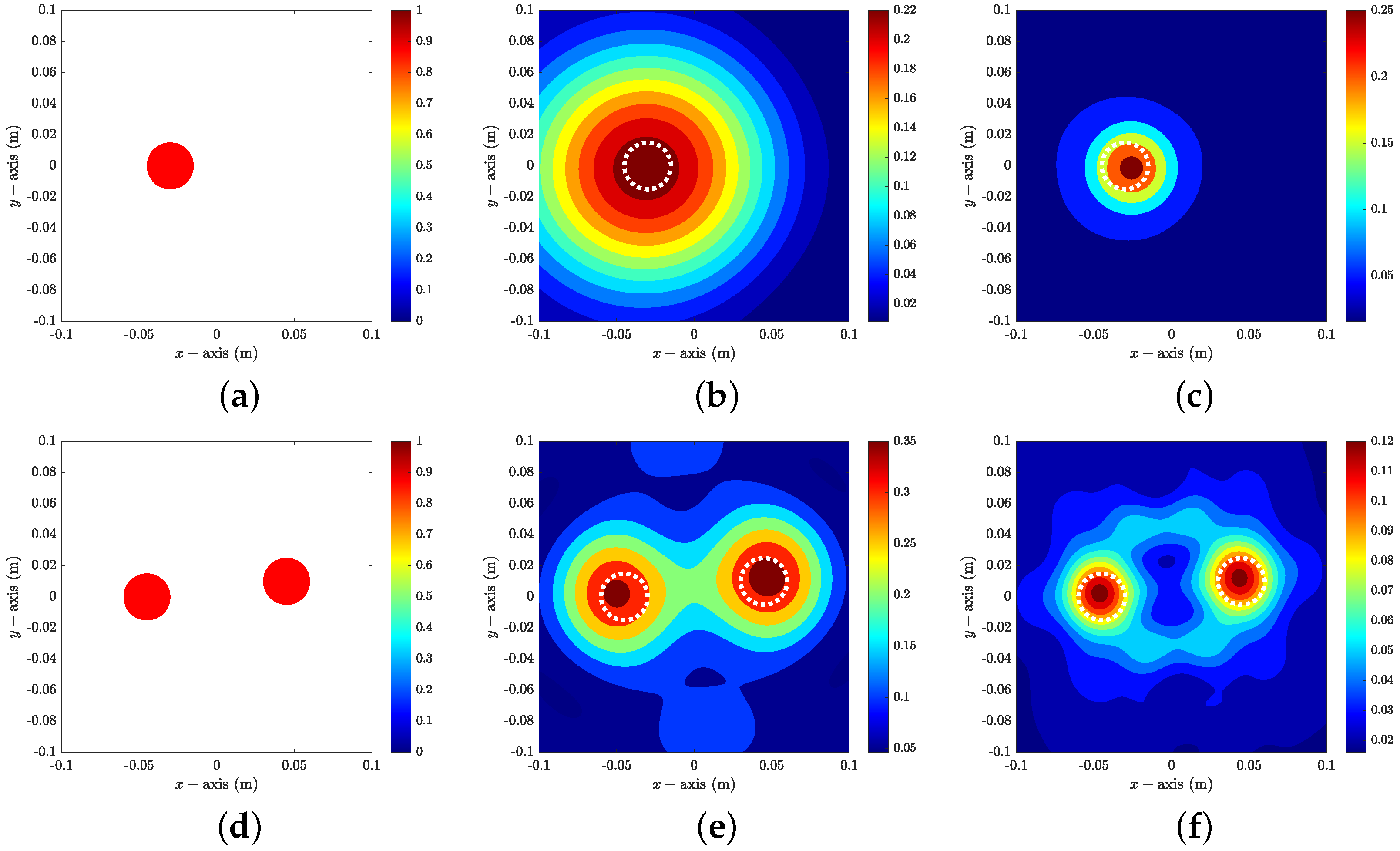
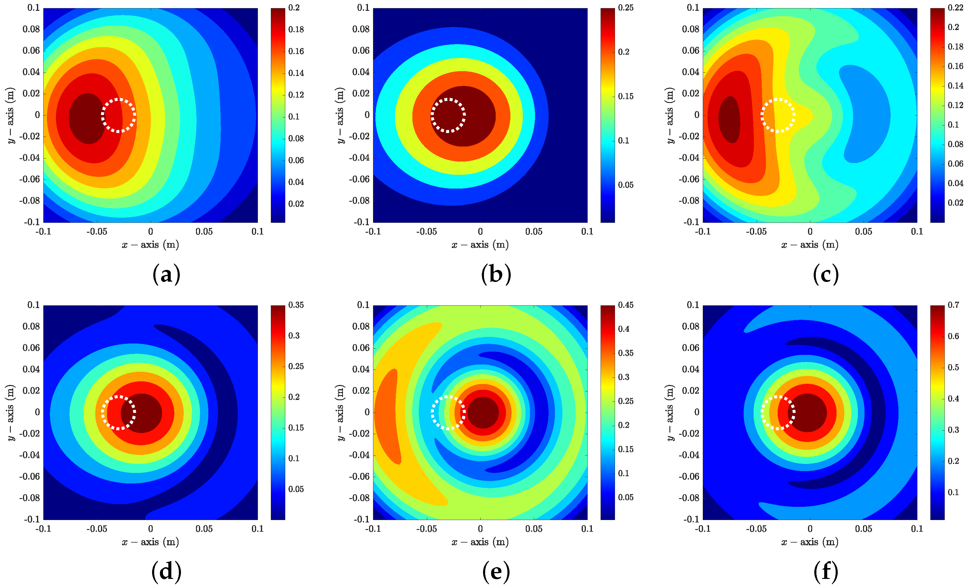
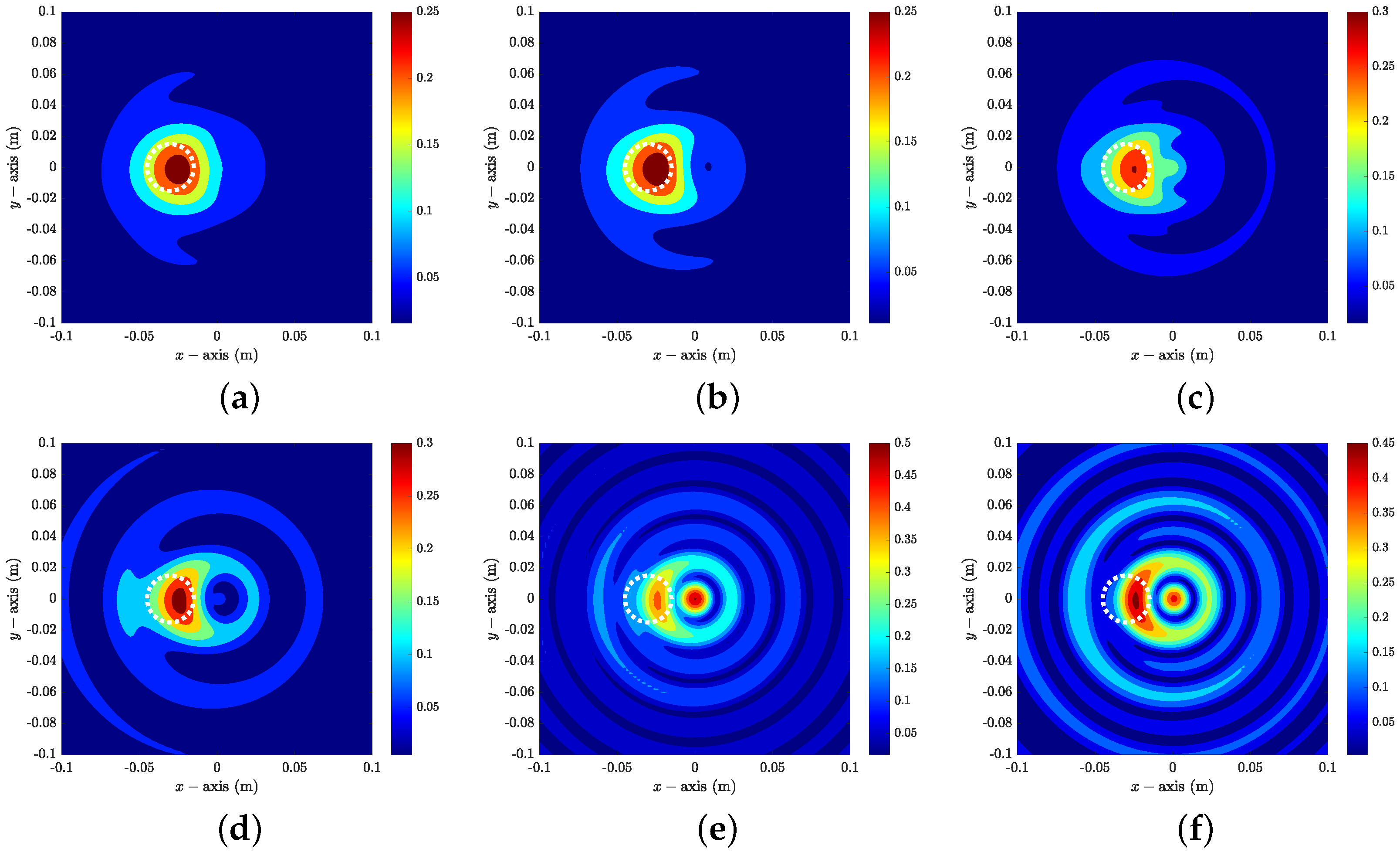
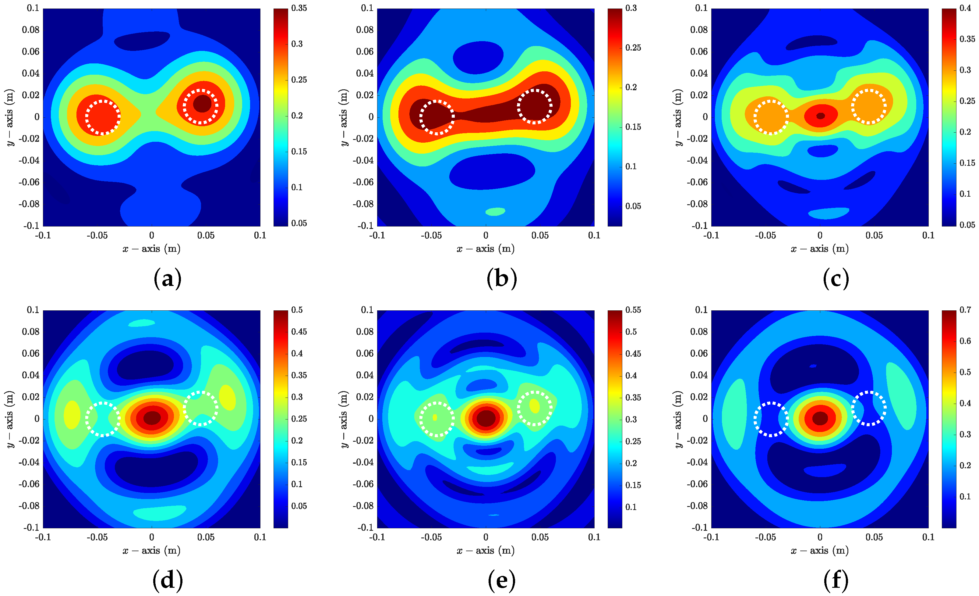
5. Simulation Results with Fresnel Dataset

Here, several numerical examples are presented and discussed to support the theoretical result and the identified properties of the KM technique. The “dielTM_dec8f.exp” dataset contains measured scattered field data in the presence of a circular object D with center $\mathbf{y}=(-0.030 \mathrm{m},0)$, radius $\alpha =0.015 \mathrm{m}$, and permittivity $\epsilon =(3\pm 0.3){\epsilon }_{\mathrm{b}}$. In addition, the “wodielTMdec8f.exp” dataset contains measured scattered field data in the presence of two circular objects $D_s$, $s=1,2$ with centers ${\mathbf{y}}_1=(-0.045 \mathrm{m},0)$, ${\mathbf{y}}_2=(0.045 \mathrm{m},0.010 \mathrm{m})$, radii ${\alpha }_s=0.015 \mathrm{m}$, and permittivities ${\epsilon }_s=(3\pm 0.3){\epsilon }_{\mathrm{b}}$. In order to show the robustness, a 20 dB white Gaussian random noise is added to the unperturbed measurement data.

Remark 1.

Note that the dataset was generated in the presence of two circular dielectric objects with the same radii and nearly the same permittivity values. Thus, differing from Discussion 4, two objects will be identified through the map of $\mathfrak{F}(\mathbf{x},0)$.

Example 1

(Imaging With Zero Constant). Figure 5 shows maps of $\mathfrak{F}(\mathbf{x},0)$ in the presence of a single object and multiple objects at $f=1,2,4,5 \mathrm{GHz}$. Based on the results, it is possible to recognize the existence, nearly accurate location, and the shape of small objects when $f=2$, 4, $5 \mathrm{GHz}$; however, it is possible to recognize the existence of D but is still difficult to identify its exact location due to the blurring effect in the imaging when $f=1 \mathrm{GHz}$. Thus, if the frequency of operation is not low, the objects were retrieved uniquely through the map of $\mathfrak{F}(\mathbf{x},0)$, which supports Discussion 3.

Example 2

(Imaging of Single Object With Nonzero Constant). Figure 6 shows maps of $\mathfrak{F}(\mathbf{x},C)$ in the presence of D at $f=1\mathrm{GHz}$. Opposite to Example 1, here, it is difficult to recognize the location and shape of D, and a large magnitude peak at the origin is included when $C=0.05i$, $0.1i$, $0.3$, and $0.3i$. Figure 7 shows maps of $\mathfrak{F}(\mathbf{x},C)$ in the presence of D at $f=4\mathrm{GHz}$. Opposite to the imaging at $f=1\mathrm{GHz}$, here, it is possible to recognize the existence, outline shape, and location of D when $\left|C\right|=0.1$ and $0.3$. However, the appearance of a large magnitude peak at the origin disturbs the identification of D when $\left|C\right|=1$.

Example 3

(Imaging of Multiple Objects With Nonzero Constant). Figure 8 shows maps of $\mathfrak{F}(\mathbf{x},C)$ in the presence of $D_1$ and $D_2$ at $f=2\mathrm{GHz}$. Opposite to Example 2, here, it is difficult to recognize the location and shape of $D_s$, and a large magnitude peak at the origin is included when $\left|C\right|\ge 0.3$. Here, two objects are recognized when $C=0.1$ but not when $C=0.1i$. In constrast to the imaging at $f=2\mathrm{GHz}$, it is possible to recognize the location of $D_1$ and $D_2$ when $f=5\mathrm{GHz}$ and $\left|C\right|=0.1$ (see Figure 9). Note that two large magnitude peaks are included in the map; however, it is very difficult to confirm the existence of two small objects because $\mathfrak{F}(\mathbf{x},C)$ reach their maximum value at the origin when $\left|C\right|\ge 0.3$.

Remark 2.

Based on the simulation results, we found that small objects can be identified through the map of $\mathfrak{F}(\mathbf{x},C)$ with a small $\left|C\right|$ value; however, it is very difficult to identify small objects with larger $\left|C\right|$ values. Note that the criteria for “small values” are ambiguous, and the selection of C is dependent on the permittivity value and the frequency of operation (refer to Discussion 2). Thus, we conclude that converting unavailable scattered field data into the zero constant is the best choice to identify small objects using the KM (refer to Discussion 3).

6. Concluding Remark

We have considered the application of the KM for fast identification of small dielectric objects from a Fresnel experimental dataset. To this end, an indicator function of the KM was designed by converting the unknown measurement data into a constant. In addition, to explain the applicability of the imaging function and the influence of the converted constant, we have demonstrated that the imaging function can be expressed by an infinite series of the Bessel functions of integer order of the first kind, the material properties, and the applied constant. Due to the theoretical result, we conclude that converting unknown measurement data into a zero constant guarantees good results and unique determination of the objects, and several simulation results were presented to verify the theoretical result.

In this study, we limited our focus to the inversion of the 2D Fresnel experimental dataset; thus, extension to the inversion of the 3D Fresnel experimental dataset [41] will be considered in future work.

References

1. Mojabi, P.; LoVetri, J. Microwave biomedical imaging using the multiplicative regularized Gauss-Newton inversion. IEEE Antennas Propag. Lett. 2009, 8, 645–648. [Google Scholar] [CrossRef]
2. Foudazix, A.; Mirala, A.; Ghasr, M.T.; Donnell, K.M. Active microwave thermography for nondestructive evaluation of surface cracks in metal structures. IEEE Trans. Instrum. Meas. 2019, 68, 576–585. [Google Scholar] [CrossRef]
3. Mallorqui, J.J.; Joachimowicz, N.; Broquetas, A.; Bolomey, J.C. Quantitative images of large biological bodies in microwave tomography by using numerical and real data. Electron. Lett. 1996, 32, 2138–2140. [Google Scholar] [CrossRef]
4. Chandra, R.; Johansson, A.J.; Gustafsson, M.; Tufvesson, F. A microwave imaging-based technique to localize an in-body RF source for biomedical applications. IEEE Trans. Biomed. Eng. 2015, 62, 1231–1241. [Google Scholar] [CrossRef]
5. Delbary, F.; Erhard, K.; Kress, R.; Potthast, R.; Schulz, J. Inverse electromagnetic scattering in a two-layered medium with an application to mine detection. Inverse Probl. 2008, 24, 015002. [Google Scholar] [CrossRef]
6. Dorn, O.; Lesselier, D. Level set methods for inverse scattering. Inverse Probl. 2006, 22, R67–R131. [Google Scholar] [CrossRef]
7. Ikeda, K.; Yoshimi, M.; Miki, C. Electrical potential drop method for evaluating crack depth. Int. J. Fract. 1991, 47, 25–38. [Google Scholar] [CrossRef]
8. Sokołowski, J.; Zochowski, A. On the topological derivative in shape optimization. SIAM J. Control Optim. 1999, 37, 1251–1272. [Google Scholar] [CrossRef]
9. Kress, R. Inverse scattering from an open arc. Math. Meth. Appl. Sci. 1995, 18, 267–293. [Google Scholar] [CrossRef]
10. Kwon, O.; Seo, J.K.; Yoon, J.R. A real-time algorithm for the location search of discontinuous conductivities with one measurement. Comm. Pur. Appl. Math. 2002, 55, 1–29. [Google Scholar] [CrossRef]
11. Park, W.K.; Lesselier, D. Reconstruction of thin electromagnetic inclusions by a level set method. Inverse Probl. 2009, 25, 085010. [Google Scholar] [CrossRef]
12. Kim, Y.J.; Jofre, L.; Flaviis, F.D.; Feng, M.Q. Microwave reflection tomographic array for damage detection of civil structures. IEEE Trans. Antennas Propag. 2003, 51, 3022–3032. [Google Scholar]
13. Jofre, L.; Broquetas, A.; Romeu, J.; Blanch, S.; Toda, A.P.; Fabregas, X.; Cardama, A. UWB tomographic radar imaging of penetrable and impenetrable objects. Proc. IEEE 2009, 97, 451–464. [Google Scholar] [CrossRef]
14. Park, W.K. Theoretical study on non-improvement of the multi-frequency direct sampling method in inverse scattering problem. Mathematics 2022, 10, 1674. [Google Scholar] [CrossRef]
15. Son, S.H.; Lee, K.J.; Park, W.K. Application and analysis of direct sampling method in real-world microwave imaging. Appl. Math. Lett. 2019, 96, 47–53. [Google Scholar] [CrossRef]
16. Boukari, Y.; Haddar, H. The factorization method applied to cracks with impedance boundary conditions. Inverse Probl. Imaging 2013, 7, 1123–1138. [Google Scholar] [CrossRef]
17. Coşğun, S.; Bilgin, E.; Çayören, M. Microwave imaging of breast cancer with factorization method: SPIONs as contrast agent. Med. Phys. 2020, 47, 3113–3122. [Google Scholar] [CrossRef]
18. Scholz, B. Towards virtual electrical breast biopsy: Space frequency MUSIC for trans-admittance data. IEEE Trans. Med. Imaging 2002, 21, 588–595. [Google Scholar] [CrossRef]
19. Park, W.K. Application of MUSIC algorithm in real-world microwave imaging of unknown anomalies from scattering matrix. Mech. Syst. Signal Proc. 2021, 153, 107501. [Google Scholar] [CrossRef]
20. Alqadah, H.F. A compressive multi-frequency linear sampling method for underwater acoustic imaging. IEEE Trans. Image Process. 2016, 25, 2444–2455. [Google Scholar] [CrossRef]
21. Audibert, L.; Haddar, H. The generalized linear sampling method for limited aperture measurements. SIAM J. Imaging Sci. 2017, 10, 845–870. [Google Scholar] [CrossRef]
22. Park, W.K. Fast localization of small inhomogeneities from far-field pattern data in limited-aperture inverse scattering problem. Mathematics 2021, 9, 2087. [Google Scholar] [CrossRef]
23. Park, W.K. Real-time detection of small anomaly from limited-aperture measurements in real-world microwave imaging. Mech. Syst. Signal Proc. 2022, 171, 108937. [Google Scholar] [CrossRef]
24. Park, W.K. Performance analysis of multi-frequency topological derivative for reconstructing perfectly conducting cracks. J. Comput. Phys. 2017, 335, 865–884. [Google Scholar] [CrossRef]
25. Muñoz, S.; Rapún, M.L. Towards flaw detection in welding joints via multi-frequency topological derivative methods. Comput. Math. Appl. 2024, 161, 121–136. [Google Scholar] [CrossRef]
26. Aprea, C.M.; Hildebrand, S.; Fehler, M.; Steck, L.; Baldridge, W.S.; Roberts, P.; Thurber, C.H.; Lutter, W.J. Three-dimensional Kirchhoff migration: Imaging of the Jemez volcanic field using teleseismic data. J. Geophys. Res. Solid Earth 2002, 107, ESE 11-1–ESE 11-15. [Google Scholar] [CrossRef]
27. Ahn, C.Y.; Ha, T.; Park, W.K. Kirchhoff migration for identifying unknown targets surrounded by random scatterers. Appl. Sci. 2019, 9, 4446. [Google Scholar] [CrossRef]
28. Bardsley, P.; Vasquez, F.G. Kirchhoff migration without phases. Inverse Probl. 2016, 32, 105006. [Google Scholar] [CrossRef]
29. Dorney, T.D.; Johnson, J.L.; Rudd, J.V.; Baraniuk, R.G.; Symes, W.W.; Mittleman, D.M. Terahertz reflection imaging using Kirchhoff migration. Opt. Lett. 2001, 26, 1513–1515. [Google Scholar] [CrossRef]
30. Park, W.K. Real-time identification of small anomalies from scattering matrix without background information. Int. J. Appl. Electromagn. Mech. 2024, 74, 289–297. [Google Scholar] [CrossRef]
31. Son, S.H.; Lee, K.J.; Park, W.K. Real-time tracking of moving objects from scattering matrix in real-world microwave imaging. AIMS Math. 2024, 9, 13570–13588. [Google Scholar] [CrossRef]
32. Zhuge, X.; Yarovoy, A.G.; Savelyev, T.; Ligthart, L. Modified Kirchhoff migration for UWB MIMO array-based radar imaging. IEEE. Trans. Geosci. Remote Sens. 2010, 48, 2692–2703. [Google Scholar] [CrossRef]
33. Kim, J.Y.; Lee, K.J.; Kim, B.R.; Jeon, S.I.; Son, S.H. Numerical and experimental assessments of focused microwave thermotherapy system at 925MHz. ETRI J. 2019, 41, 850–862. [Google Scholar] [CrossRef]
34. Belkebir, K.; Saillard, M. Special section: Testing inversion algorithms against experimental data. Inverse Probl. 2001, 17, 1565–1571. [Google Scholar] [CrossRef]
35. Ammari, H.; Kang, H. Reconstruction of Small Inhomogeneities from Boundary Measurements; Lecture Notes in Mathematics; Springer: Berlin/Heidelberg, Germany, 2004; Volume 1846. [Google Scholar]
36. Bleistein, N.; Cohen, J.; Stockwell, J.S., Jr. Mathematics of Multidimensional Seismic Imaging, Migration, and Inversion; Interdisciplinary Applied Mathematics; Springer: New York, NY, USA, 2001; Volume 13. [Google Scholar]
37. Ammari, H.; Garnier, J.; Kang, H.; Park, W.K.; Sølna, K. Imaging schemes for perfectly conducting cracks. SIAM J. Appl. Math. 2011, 71, 68–91. [Google Scholar] [CrossRef]
38. Eom, J.; Park, W.K. Real-time detection of small objects in transverse electric polarization: Evaluations on synthetic and experimental datasets. AIMS Math. 2024, 9, 22665–22679. [Google Scholar] [CrossRef]
39. Colton, D.; Kress, R. Inverse Acoustic and Electromagnetic Scattering Problems; Mathematics and Applications Series; Springer: New York, NY, USA, 1998; Volume 93. [Google Scholar]
40. Park, W.K. Multi-frequency subspace migration for imaging of perfectly conducting, arc-like cracks in full- and limited-view inverse scattering problems. J. Comput. Phys. 2015, 283, 52–80. [Google Scholar] [CrossRef]
41. Geffrin, J.M.; Sabouroux, P.; Eyraud, C. Free space experimental scattering database continuation: Experimental set-up and measurement precision. Inverse Probl. 2005, 21, S117–S130. [Google Scholar] [CrossRef]
Figure 1. Receiver arrangements corresponding to the transmitter location.
Mathematics 12 03253 g001
Figure 2. Visualization of the modulus of M ( C ) : (a) C = 0 , (b) C = 0.05 , and (c) C = 0.1 .
Mathematics 12 03253 g002
Figure 3. 1D plots of Φ ( x , 0 ) at f = 2 , 5 , 10   GHz .
Mathematics 12 03253 g003
Figure 4. 1D plots of Ψ ( x ) at f = 2 , 5 , 10   GHz .
Mathematics 12 03253 g004
Figure 5. (a) illustration of single object; (b) map of F ( x , 0 ) at 1   GHz ; (c) map of F ( x , 0 ) at 4   GHz ; (d) illustration of multiple objects; (e) map of F ( x , 0 ) at 2   GHz ; (f) map of F ( x , 0 ) at 5   GHz . The white dashed lines describe the boundaries of the objects.
Mathematics 12 03253 g005
Figure 6. Maps of F ( x , C ) at 1   GHz : (a) C = 0.05 ; (b) C = 0.05 i ; (c) C = 0.1 ; (d) C = 0.1 i ; (e) C = 0.3 ; (f) C = 0.3 i . The white dashed lines describe the boundaries of the objects.
Mathematics 12 03253 g006
Figure 7. Maps of F ( x , C ) at 4   GHz : (a) C = 0.1 ; (b) C = 0.1 i ; (c) C = 0.3 ; (d) C = 0.3 i ; (e) C = 1 ; (f) C = 1 i . The white dashed lines describe the boundaries of the objects.
Mathematics 12 03253 g007
Figure 8. Maps of F ( x , C ) at 2   GHz : (a) C = 0.1 ; (b) C = 0.1 i ; (c) C = 0.3 ; (d) C = 0.3 i ; (e) C = 0.5 ; (f) C = 0.5 i . The white dashed lines describe the boundaries of the objects.
Mathematics 12 03253 g008
Figure 9. Maps of F ( x , C ) at 5   GHz : (a) C = 0.1 ; (b) C = 0.1 i ; (c) C = 0.3 ; (d) C = 0.3 i ; (e) C = 0.5 ; (f) C = 0.5 i . The white dashed lines describe the boundaries of the objects.
Mathematics 12 03253 g009
Disclaimer/Publisher’s Note: The statements, opinions and data contained in all publications are solely those of the individual author(s) and contributor(s) and not of MDPI and/or the editor(s). MDPI and/or the editor(s) disclaim responsibility for any injury to people or property resulting from any ideas, methods, instructions or products referred to in the content.