Pricing of a Binary Option Under a Mixed Exponential Jump Diffusion Model

Abstract

This paper focuses on the pricing problem of binary options under stochastic interest rates, stochastic volatility, and a mixed exponential jump diffusion model. Considering the negative interest rates in the market in recent years, this paper assumes that the stochastic interest rate follows the Hull–White (HW) model. In addition, we assume that the stochastic volatility follows the Heston volatility model, and the price of the underlying asset follows the jump diffusion model in which the jumps follow the mixed exponential jump model. Considering these factors comprehensively, the mixed exponential jump diffusion of the Heston–HW (abbreviated as MEJ-Heston–HW) model is established. Using the idea of measure transformation, the pricing formula of binary call options is derived by the martingale method, eigenfunction, and Fourier transform. Finally, the effects of the volatility term and the parameters of the mixed-exponential jump diffusion model on the option price in the O-U process are analyzed. In the numerical simulation, compared with the double exponential jump Heston–HW (abbreviated as DEJ-Heston–HW) model and the Heston–HW model, the mixed exponential jump model is an extension of the double exponential jump model, which can approximate any distribution in the sense of weak convergence, including arbitrary discrete distributions, normal distributions, and various thick-tailed distributions. Therefore, the MEJ-Heston–HW model adopted in this paper can better describe the price of the underlying asset.

1. Introduction

A binary option, also known as a digital option, is an exotic option with discontinuous payoffs, where the holder can obtain a pre-determined fixed amount of money if the underlying asset exceeds the finalized price on expiration date T, or nothing at all otherwise. The gain and loss structure of binary options is predefined, so that investors can better control the risk. Due to the nature of the binary option itself, investors do not need to go through in-depth research and evaluation to accurately predict the price changes in the underlying asset, and can establish a larger trading position with a minimum investment amount flow.

Black et al. [1] pioneered the derivation of a pricing formula for European options, which laid the foundation of a paradigm for the study of option pricing problems. It assumes that the stock price satisfies geometric Brownian motion, and expected return rate and volatility are fixed constants. Rubinstein et al. [2] derived the pricing formula for binary options under the Black–Scholes model (hereafter referred to as the BS model). In the BS model, the interest rate and the volatility are both constants.

In recent years, many scholars have found that the price fluctuation of financial assets is a biased random walk, and the return rate of assets does not follow the normal distribution, but show the phenomenon of “peak and thick tail” [3]. To better depict these features, many scholars change the assumption that the interest rate and volatility are constant on the basis of BS model, and add the jump process to better depict the nature of assets themselves.

Heston [4] assumed that the volatility was consistent with the stochastic differential equation, and the closed solution of the European option was obtained under the single factor stochastic volatility model. The model in this paper is the classical Heston volatility model used by many scholars. On the basis of this classic model, scholars have made many improvements. Da Fonseca et al. [5] extended the Heston model to a multi-factor volatility model, and proved the applicability of the extended multi-factor volatility. He et al. [6] obtained the analytical formula of European option pricing under the mixed model, and that the volatility of Heston volatility model follows Markov chain.

In addition to volatility, the stochastic interest rate is also a significant risk term; the most commonly used interest rate model is the Vasicek model [7]. However, the parameters of Vasicek model are constant. Cox et al. [8] used the square root process of mean reversion to model interest rates and proposed a non-negative CIR interest rate model. Hull et al. [9] proposed a Hull–White model where the parameter is a function and the interest rate may be negative. Considering the negative interest rate in some areas in recent years, the HW model is adopted in this paper to describe the actual interest rate.

Meanwhile, it is one of the current research trends to add the jump diffusion model to the option pricing model to describe the jump situation of underlying asset prices. The jump diffusion model was first introduced into option pricing by Merton [10], who adopted a compound Poisson process to simulate discontinuous changes in stock prices. Kou [11] proposed a double exponential jump-diffusion (DEJ) model. On the basis of DEJ model, Cai et al. [12] proposed a mixed exponential jump diffusion (MEJ) model, it is a weighted average of the exponential distribution, and the weights may be negative. It can approximate any distribution in the sense of weak convergence, including arbitrary discrete distributions, normal distributions, and various thick-tailed distributions, such as the gamma, Weibull, and Pareto distributions. In order to better characterize the changes in the underlying assets, this paper adopts the MEJ model, and assumes that the interest rate follows the HW model, and the volatility follows the Heston model. The Heston–HW model with mixed exponential jump diffusion is established.

Binary options are popular in the Over-The-Counter market, and are a fundamental tool in the construction of more complex options products. It has aroused the interest of many scholars to study binary options. Kolková et al. [13] introduced the significance of binary options as a modern financial instrument. Liu et al. [14] applied the martingale method to the binary option pricing problem, and the pricing formula for the binary fragile options under stochastic interest rates was solved. Thavaneswaran et al. [15] used fuzzy theory to price binary options, and obtained option pricing formulas for different price intervals. He et al. [16] studied Monte Carlo methods for pricing binary options on credit default swaps under regime switching. Gao [17] studied British binary options, and derived a closed expression for the no-arbitrage price using the ideal strike boundary condition. Qin et al. [18] investigated the pricing of binary options in a fuzzy environment. Nikita [19] examined binary barrier option pricing, and gave a formula for binary barrier option pricing in a financial market model. Yang et al. [20] derived an explicit pricing formula for binary options under uncertainty theory.

The existing literature has not involved research on the pricing problem of binary options under the model that the price of underlying assets obey the mixed-exponential jump, stochastic volatility, and stochastic interest rate. In addition, due to the impact of the COVID-19 epidemic, the interest rate is negative in some countries and regions. Therefore, it is necessary to study the pricing problem of binary options under the MEJ-Heston–HW model.

In summary, this paper investigates the pricing problem of binary call options under the MEJ-Heston–HW model, and obtains the pricing formula of binary call options using the Fourier transform method. The results obtained in this paper generalize the existing related conclusions about binary option pricing, and have certain theoretical and practical significance.

2. Model Assumptions

Given the complete probability space $(\mathsf{\Omega },\mathcal{F},{\mathcal{F}}_t,Q)$, ${\mathcal{F}}_t$ is the $\sigma$-algebraic flow, Q is the neutral risk measure, and all stochastic processes in this paper are measurable in this probability space.

Assume that the interest rate $\{r_t,0\le t\le T\}$ obeys the following HW interest rate model:

$$d{r}_t=k(\theta -r_t)dt+{\sigma }_{r}d{B}_r\left(t\right),$$

(1)

where $\{B_r\left(t\right),0\le t\le T\}$ is the standard Brownian motion, $\theta$ is the long-term mean, k is the tensile velocity, and k, $\theta$, and ${\sigma }_r$ are all positive constants. When the interest rate deviates from $\theta$, it will converges to $\theta$ at a rate k.

Assume that the stochastic volatility $\{v_t,0\le t\le T\}$ obeys the following Heston volatility model:

$$d{v}_t=\alpha \left(\beta -v_t\right)dt+{\sigma }_v\sqrt{v_t}d{B}_v\left(t\right)$$

(2)

where $\{B_v\left(t\right),0\le t\le T\}$ is the standard Brownian motion, $\alpha$ is the tensile velocity, $\beta$ is the long term mean, ${\sigma }_v$ is the volatility coefficient, and ${\sigma }_v$, $\alpha$, and $\beta$ are all positive constants that satisfy Feller condition $2\alpha \beta >{{\sigma }_v}^2$, which ensures that the process $\{v_t,0\le t\le T\}$ is strictly positive when started from any positive value.

Assume that the jump-diffusion process of the underlying asset $\{S_t,0\le t\le T\}$ satisfies

$$d{S}_t=S_t\left(r_t-\lambda h\right)dt+S_t\sqrt{v_t}dB\left(t\right)+S_t\left(j-1\right)dN\left(t\right),$$

(3)

where $\left\{B\right(t),0\le t\le T\}$ is the standard Brownian motion, $\left\{N\right(t),0\le t\le T\}$ is the Poisson process with intensity $\lambda$, $h=E(j-1)$, and j is the jump intensity of the underlying asset.

According to $It$$\widehat{o}$ Lemma [21] and Theorem 8.33 [22], Equation (3) can be rewritten as

$$ln{S}_T=ln{S}_t+{\int }_t^T(r_s-\lambda h-{\displaystyle \frac{v_s}{2}})ds+{\int }_t^T\sqrt{v_s}dB\left(s\right)+\sum _{\mathrm{i}=1}^{N_{T-t}}{Z}_{\mathrm{i}},$$

(4)

where $Z=ln\left(j\right)$. Assume that Z is a random variable obeying a mixed exponential distribution, and its probability density is

$$f_Z\left(z\right)=p_u\sum _{k_1=1}^m{p}_{k_1}{\eta }_{k_1}{e}^{-{\eta }_{k_1}z}{I}_{\{z\ge 0\}}+q_d\sum _{k_2=1}^n{q}_{k_2}{\theta }_{k_2}{e}^{-{\theta }_{k_2}z}{I}_{\{z<0\}}.$$

(5)

Here is a mixture of m exponential distributions on the positive semiaxis and n exponential distributions on the negative semiaxis, the probability of a positive jump is $p_u\ge 0$, the probability of a negative jump is $q_d=1-p_u\ge 0$, the weight ratio of each index in the mixed index satisfies ${\sum }_{k_1=1}^m{p}_{k_1}={\sum }_{k_2=1}^n{q}_{k_2}=1$, and ${\eta }_{k_1}$ and ${\theta }_{k_2}$ are the parameters of each index distribution, which satisfy the following constraints:

$$\left\{\begin{array}{c}{\sum }_{k_1=1}^{U_1}{p}_{k_1}{\eta }_{k_1}\ge 0,\forall U_1=1,2,\cdots ,m,\hfill \\ {\sum }_{k_2=1}^{U_2}{q}_{k_2}{\theta }_{k_2}\ge 0,\forall U_2=1,2,\cdots ,n,\hfill \\ {\eta }_{k_1}>1,\forall k_1=1,2,\cdots ,m,\hfill \\ {\theta }_{k_2}>0,\forall k_2=1,2,\cdots ,n.\hfill \end{array}\right.$$

(6)

According to Equations (1)–(6), we establish the MEJ-Heston–HW model of this paper as

$$\left\{\begin{array}{c}d{S}_t=S_t\left(r_t-\lambda h\right)dt+S_t\sqrt{v_t}dB\left(t\right)+S_t\left(j-1\right)dN\left(t\right),\hfill \\ d{r}_t=k\left(\theta -r_t\right)dt+{\sigma }_{r}d{B}_r\left(t\right),\hfill \\ d{v}_t=\alpha \left(\beta -v_t\right)dt+{\sigma }_v\sqrt{v_t}d{B}_v\left(t\right).\hfill \end{array}\right.$$

(7)

where $\left\{B\right(t),0\le t\le T\}$, $\{B_r\left(t\right),0\le t\le T\}$, $\{B_v\left(t\right),0\le t\le T\}$, and $\{N_t,0\le t\le T\}$ are all independent of each other.

3. Pricing Formulas for Binary Call Option Under the MEJ-Heston–HW Model

There are two typical types of binary call options: cash-or-nothing call options (abbreviated as CONC) and asset-or nothing-call options (abbreviated as ANOC); their value at the expiration date T are defined by

$$V\left(T\right)=\left\{\begin{array}{c}{S}_{T}H(S_T-K),\left(ANOC\right)\hfill \\ H(S_T-K),\left(CNOC\right)\hfill \end{array}\right.$$

(8)

where $H\left(x\right)$ is the Heviside function, i.e., $H\left(x\right)=\left\{\begin{array}{c}1,x>0\hfill \\ 0,x\le 0\hfill \end{array}\right.$. In the following, $V_A$ and $V_C$ denote the price of ANOC and CONC, respectively.

The pricing formula of $V_A$ for a binary option under the MEJ-Heston–HW model is given below.

Theorem 1.

If the financial market satisfies the modeling assumptions in Equation (7), the price of the asset or worthless call option $V_A\left(t\right)$ at time $t\in [0,T]$ is

$$\begin{array}{c}\hfill V_A\left(t\right)=S_t\left({\displaystyle \frac{1}{2}}+{\displaystyle \frac{1}{\pi }}{\int }_0^{+\infty }Real\left[{\displaystyle \frac{{\varphi }_1\left(u\right){\mathrm{e}}^{-iulnK}}{iu}}\right]du\right),\end{array}$$

where

$$\begin{array}{cc}& \tau =(T-t),\hfill \\ & {\varphi }_1\left(u\right)={\displaystyle \frac{e^{(iu+1)ln{S}_t-\lambda h(iu+1)\tau }{\mathrm{e}}^{A\left(t\right)+B\left(t\right)v+C\left(t\right)+D\left(t\right)r+\lambda \tau \left(p_u{\sum }_{k_1=1}^m\frac{p_{k_1}{\eta }_{k_1}}{{\eta }_{k_1}-iu}+q_d{\sum }_{k_2=1}^n\frac{q_{k_2}{\theta }_{k_2}}{{\theta }_{k_2}+iu}-1\right)}}{S_t}},\hfill \\ & A\left(t\right)={\displaystyle \frac{\alpha \beta c_1}{2{{\sigma }_v}^{2}c}}ln\left({\displaystyle \frac{m_1{\mathrm{e}}^{-2c\tau }+1}{m_1+1}}\right)+{\displaystyle \frac{m_1\alpha \beta c_1}{2{{\sigma }_v}^{2}c}}ln\left({\displaystyle \frac{m_1{\mathrm{e}}^{-2c\tau }+1}{{\mathrm{e}}^{-2c\tau }(m_1+1)}}\right)\hfill \\ & B\left(t\right)={\displaystyle \frac{-c_1{\mathrm{e}}^{-2c\tau }-1}{{{\sigma }_v}^2({\mathrm{e}}^{-2c\tau }-1+\frac{2c}{c_2})}},\hfill \\ & C\left(t\right)=-{\displaystyle \frac{{\sigma }_r^2}{4k}}\left[{\mathrm{e}}^{-2k\tau }-1\right]+{\displaystyle \frac{{\sigma }_r^2+iu{k}^2\theta }{k^3}}\left[{\mathrm{e}}^{-k\tau }-1\right]+\left({\displaystyle \frac{{\sigma }_r^2{\left(iu\right)}^2-2k^2\theta iu}{2k^2}}\right)\tau ,\hfill \\ & D\left(t\right)=-{\displaystyle \frac{iu}{k}}({\mathrm{e}}^{-k\tau }-1),\hfill \\ & m_1={\displaystyle \frac{c_2}{2c-c_2}},\hfill \\ & c=\sqrt{{\alpha }^2-({(iu+1)}^2-(iu+1)){\sigma }_v^2},\hfill \\ & c_1=-\alpha -c,c_2=-\alpha +c.\hfill \end{array}$$

Proof of Theorem 1. 

Similarly to [23], the risk-neutral measure Q can be transformed into the measure $Q_1$ by the Radon–Nikodym derivative

$${\displaystyle \frac{d{Q}_1}{dQ}}\mid {\mathcal{F}}_t={\mathrm{e}}^{-{\int }_t^T{r}_{s}ds}{\displaystyle \frac{S_T}{S_t}}.$$

(9)

By Girsanov’s theorem, $Q_1$ is a probability measure, and is equivalent to Q. So, we obtain

$$\begin{array}{cc}\hfill V_A\left(t\right)& =E^Q\left[{\mathrm{e}}^{-{\int }_t^T{r}_{s}ds}{S}_{T}H(S_T-K)\mid {\mathcal{F}}_t\right]\hfill \\ & =S_t{E}^{Q_1}[H(S_T-K)\mid {\mathcal{F}}_t]\hfill \\ & =S_t{Q}_{1}H(S_T-K)\hfill \\ & =S_t{Q}_1(ln{S}_T>lnK).\hfill \end{array}$$

(10)

In the following, the closed-form solution of the probability $Q_1(ln{S}_T>lnK)$ is obtained by the unique deterministic relation between the characteristic function and the distribution function. First, let us find the eigenfunction of $ln{S}_T$, i.e.,

$${\varphi }_1\left(u\right)=E^{Q_1}\left[{\mathrm{e}}^{iuln{S}_T}\mid {\mathcal{F}}_t\right].$$

(11)

The Fourier inverse transform gives

$$Q_1(ln{S}_T>lnK)={\displaystyle \frac{1}{2}}+{\displaystyle \frac{1}{\pi }}{\int }_0^{+\infty }Real\left[{\displaystyle \frac{{\varphi }_1\left(u\right){\mathrm{e}}^{-iulnK}}{iu}}\right]du.$$

(12)

Substituting Equation (4) into Equation (11) yields

$$\begin{array}{c}\hfill E^{Q_1}\left[{\mathrm{e}}^{iuln{S}_T}\mid {\mathcal{F}}_t\right]=E^{Q_1}\left[{\mathrm{e}}^{iu(ln{S}_t+{\int }_t^T(r_s-\lambda h-{\displaystyle \frac{v_s}{2}})ds+{\int }_t^T\sqrt{v_s}dB\left(s\right)+{\sum }_{\mathrm{i}=1}^{N_{T-t}}{Z}_{\mathrm{i}})}\mid {\mathcal{F}}_t\right].\end{array}$$

By means of the measure transformation, we can obtain

$$\begin{array}{cc}\hfill & E^{Q_1}\left[{\mathrm{e}}^{iuln{S}_T}\mid {\mathcal{F}}_t\right]\hfill \\ \hfill & =E^Q\left[{\displaystyle \frac{S_T}{S_t}}{\mathrm{e}}^{-{\int }_t^T{r}_{s}ds}{\mathrm{e}}^{iu(ln{S}_t+{\int }_t^T(r_s-\lambda h-{\displaystyle \frac{v_s}{2}})ds+{\int }_t^T\sqrt{v_s}dB\left(s\right)+{\sum }_{\mathrm{i}=1}^{N_{T-t}}{Z}_{\mathrm{i}})}\mid {\mathcal{F}}_t\right]\hfill \\ \hfill & ={\displaystyle \frac{1}{S_t}}{E}^Q\left[{\mathrm{e}}^{-{\int }_t^T{r}_{s}ds}{\mathrm{e}}^{(iu+1)(ln{S}_t+{\int }_t^T(r_s-\lambda h-{\displaystyle \frac{v_s}{2}})ds+{\int }_t^T\sqrt{v_s}dB\left(s\right)+{\sum }_{\mathrm{i}=1}^{N_{T-t}}{Z}_{\mathrm{i}})}\mid {\mathcal{F}}_t\right]\hfill \\ \hfill & ={\varphi }_1\left(u\right).\hfill \end{array}$$

(13)

In the following, we calculate $E^Q[{\mathrm{e}}^{{\displaystyle \frac{1}{2}}({(iu+1)}^2-(iu+1)){\int }_t^T{v}_{s}ds}\mid {\mathcal{F}}_t]$ firstly, and let

$$E^Q\left[{\mathrm{e}}^{{\displaystyle \frac{1}{2}}({(iu+1)}^2-(iu+1)){\int }_t^T{v}_{s}ds}\mid {\mathcal{F}}_t\right]=g(v,t),$$

(14)

We will prove that ${\mathrm{e}}^{{\displaystyle \frac{1}{2}}({(iu+1)}^2-(iu+1)){\int }_0^t{v}_{s}ds}g(v,t)$ is a martingale. In fact, for $0\le t_1\le t\le T$, we have

$$\begin{array}{cc}\hfill & E^Q\left[E^Q\left[{\mathrm{e}}^{{\displaystyle \frac{1}{2}}({(iu+1)}^2-(iu+1)){\int }_0^t{v}_{s}ds}{\mathrm{e}}^{{\displaystyle \frac{1}{2}}({(iu+1)}^2-(iu+1)){\int }_t^T{v}_{s}ds}\mid {\mathcal{F}}_t\right]\mid {\mathcal{F}}_{t_1}\right]\hfill \\ \hfill & =E^Q\left[{\mathrm{e}}^{{\displaystyle \frac{1}{2}}({(iu+1)}^2-(iu+1)){\int }_0^T{v}_{s}ds}\mid {\mathcal{F}}_{t_1}\right]\hfill \\ \hfill & ={\mathrm{e}}^{{\displaystyle \frac{1}{2}}({(iu+1)}^2-(iu+1)){\int }_0^{t_1}{v}_{s}ds}{E}^Q\left[{\mathrm{e}}^{{\displaystyle \frac{1}{2}}({(iu+1)}^2-(iu+1)){\int }_{t_1}^T{v}_{s}ds}\mid {\mathcal{F}}_{t_1}\right]\hfill \\ \hfill & ={\mathrm{e}}^{{\displaystyle \frac{1}{2}}({(iu+1)}^2-(iu+1)){\int }_0^{t_1}{v}_{s}ds}g(v,t_1).\hfill \end{array}$$

According to the $It$$\widehat{o}$ lemma, for the differential form of ${\mathrm{e}}^{{\displaystyle \frac{1}{2}}({(iu+1)}^2-(iu+1)){\int }_0^t{v}_{s}ds}g(v,t)$ we have

$$\begin{array}{cc}\hfill & d{\mathrm{e}}^{{\displaystyle \frac{1}{2}}({(iu+1)}^2-(iu+1)){\int }_0^t{v}_{s}ds}g(v,t)\hfill \\ \hfill & =g(v,t)d{\mathrm{e}}^{{\displaystyle \frac{1}{2}}({(iu+1)}^2-(iu+1)){\int }_0^t{v}_{s}ds}+{\mathrm{e}}^{{\displaystyle \frac{1}{2}}({(iu+1)}^2-(iu+1)){\int }_0^t{v}_{s}ds}dg(v,t)\hfill \\ \hfill & ={\mathrm{e}}^{{\displaystyle \frac{1}{2}}({(iu+1)}^2-(iu+1)){\int }_0^t{v}_{s}ds}\left[{\displaystyle \frac{\partial g}{\partial t}}dt+{\displaystyle \frac{\partial g}{\partial v}}dv+{\displaystyle \frac{1}{2}}{\displaystyle \frac{{\partial }^{2}g}{\partial v^2}}{\left(dv\right)}^2\right]\hfill \\ \hfill & +{\mathrm{e}}^{{\displaystyle \frac{1}{2}}\left({(iu+1)}^2-(iu+1)\right){\int }_0^t{v}_{s}ds}{\displaystyle \frac{1}{2}}\left({(iu+1)}^2-1\right)g(v,t)vdt\hfill \\ \hfill & ={\mathrm{e}}^{{\displaystyle \frac{1}{2}}({(iu+1)}^2-(iu+1)){\int }_0^t{v}_{s}ds}[\left(\left({\displaystyle \frac{\partial g}{\partial t}}+{\displaystyle \frac{1}{2}}({(iu+1)}^2-(iu+1\right)\right)g(v,t)v+{\displaystyle \frac{1}{2}}{\displaystyle \frac{{\partial }^{2}g}{\partial v^2}}{{\sigma }_v}^{2}v\hfill \\ \hfill & +{\displaystyle \frac{\partial g}{\partial v}}\left(\alpha (\beta -v)\right))dt+{\sigma }_v\sqrt{v}{\displaystyle \frac{\partial g}{\partial v}}d{B}^v\left(t\right)].\hfill \end{array}$$

By the the proposition of the martingale that a continuous finite-variation martingale with initial value 0 is 0, the drift term in the differential form of martingale is 0, and we can obtain

$$\left\{\begin{array}{c}{\displaystyle \frac{\partial g}{\partial t}}+{\displaystyle \frac{1}{2}}\left({(iu+1)}^2-(iu+1)\right)g(v,t)v+{\displaystyle \frac{1}{2}}{\displaystyle \frac{{\partial }^{2}g}{\partial v^2}}{{\sigma }_r}^{2}v+{\displaystyle \frac{\partial g}{\partial v}}\alpha (\beta -v)=0,\hfill \\ g(v,T)=1.\hfill \end{array}\right.$$

(15)

Based on Duffie’s idea of the affine structure solution, let

$$g(v,t)={\mathrm{e}}^{A\left(t\right)+B\left(t\right)v}.$$

(16)

Substituting Equation (16) into Equation (15) gives the following equations:

$$\left\{\begin{array}{c}{\displaystyle \frac{dA}{dt}}+B\alpha \beta =0,\hfill \\ {\displaystyle \frac{dB}{dt}}+{\displaystyle \frac{1}{2}}\left({(iu+1)}^2-(iu+1)\right)+{\displaystyle \frac{1}{2}}{B}^2{{\sigma }_v}^2-\alpha \beta =0.\hfill \end{array}\right.$$

(17)

According to $g(v,T)=1$, we can know the terminal value condition $A\left(T\right)=B\left(T\right)=0$, and substituting into Equation (17), we obtain

$$B\left(t\right)={\displaystyle \frac{-c_1({\mathrm{e}}^{-2c\tau }-1)}{{{\sigma }_v}^2\left({\mathrm{e}}^{-2c\tau }-1+\frac{2c}{c_2}\right)}}.$$

(18)

and

$$A\left(t\right)={\displaystyle \frac{\alpha \beta c_1}{2{{\sigma }_v}^{2}c}}ln\left({\displaystyle \frac{m_1{\mathrm{e}}^{-2c\tau }+1}{m_1+1}}\right)+{\displaystyle \frac{m_1\alpha \beta c_1}{2{{\sigma }_v}^{2}c}}ln\left({\displaystyle \frac{m_1{\mathrm{e}}^{-2c\tau }+1}{m_1+1}}\right).$$

(19)

Then, we will solve for the stochastic interest rate part below. Let

$$E^Q\left[{\mathrm{e}}^{iu{\int }_t^T{r}_{s}ds}\mid {\mathcal{F}}_t\right]=f(r,t).$$

(20)

We will prove that ${\mathrm{e}}^{iu{\int }_0^t{r}_{s}ds}f(r,t)$ is a martingale. In fact, for $0\le t_1\le t\le T$, we have

$$\begin{array}{cc}\hfill & E^Q\left[{\mathrm{e}}^{iu{\int }_t^T{r}_{s}ds}\mid {\mathcal{F}}_{t_1}\right]\hfill \\ \hfill & =E^Q\left[E^Q\left[{\mathrm{e}}^{iu{\int }_0^T{r}_{s}ds}{\mathrm{e}}^{iu{\int }_t^T{r}_{s}ds}\mid {\mathcal{F}}_t\right]\mid {\mathcal{F}}_{t_1}\right]\hfill \\ \hfill & ={\mathrm{e}}^{iu{\int }_0^{t_1}{r}_{s}ds}{E}^Q\left[{\mathrm{e}}^{iu{\int }_{t_1}^T{r}_{s}ds}\mid {\mathcal{F}}_{t_1}\right]\hfill \\ \hfill & ={\mathrm{e}}^{iu{\int }_0^{t_1}{r}_{s}ds}f(r,t_1).\hfill \end{array}$$

According to the $It$$\widehat{o}$ lemma, for the differential form of ${\mathrm{e}}^{iu{\int }_0^t{r}_{s}ds}f(r,t)$, we have

$$\begin{array}{cc}\hfill & d{\mathrm{e}}^{iu{\int }_0^t{r}_{s}ds}f(r,t)\hfill \\ \hfill & =f(r,t)d{\mathrm{e}}^{iu{\int }_0^t{r}_{s}ds}+{\mathrm{e}}^{iu{\int }_0^t{r}_{s}ds}df(r,t)\hfill \\ \hfill & ={\mathrm{e}}^{iu{\int }_0^t{r}_{s}ds}\left[{\displaystyle \frac{\partial f}{\partial t}}dt+{\displaystyle \frac{\partial f}{\partial r}}dr+{\displaystyle \frac{1}{2}}{\displaystyle \frac{{\partial }^{2}f}{\partial r^2}}{\left(dr\right)}^2\right]+{\mathrm{e}}^{iu{\int }_0^t{r}_{s}ds}iuf(r,t)rdt\hfill \\ \hfill & ={\mathrm{e}}^{iu{\int }_0^t{r}_{s}ds}\left[{\displaystyle \frac{\partial f}{\partial t}}+{\displaystyle \frac{1}{2}}{\displaystyle \frac{{\partial }^{2}f}{\partial r^2}}{{\sigma }_r}^2+{\displaystyle \frac{\partial f}{\partial r}}k(\theta -r)+iuf(r,t)r\right]dt+{\mathrm{e}}^{iu{\int }_0^t{r}_{s}ds}{\displaystyle \frac{\partial f}{\partial r}}{\sigma }_{r}d{B}_r\left(t\right)dt,\hfill \end{array}$$

When $t=T$, $f(r,T)=1$, by the proposition of the martingale, the drift term in the differential form of ${\mathrm{e}}^{iu{\int }_0^t{r}_{s}ds}f(r,t)$ is 0, so we can obtain the following PDE equation:

$$\left\{\begin{array}{c}{\displaystyle \frac{\partial f}{\partial t}}+{\displaystyle \frac{1}{2}}{\displaystyle \frac{{\partial }^{2}f}{\partial r^2}}{{\sigma }_r}^{2}v+{\displaystyle \frac{\partial f}{\partial r}}k(\theta -r)+iuf(r,t)=0,\hfill \\ f(r,T)=1.\hfill \end{array}\right.$$

(21)

According to Duffie’s idea of an affine structure solution, let

$$f(r,t)={\mathrm{e}}^{C\left(t\right)+D\left(t\right)r}.$$

(22)

Substituting Equation (22) into Equation (21), we can obtain the following ODE:

$$\left\{\begin{array}{c}{\displaystyle \frac{\mathrm{d}C}{\mathrm{d}t}}+{\displaystyle \frac{1}{2}}{D}^2{{\sigma }_r}^2+Dk\theta =0,\hfill \\ {\displaystyle \frac{\mathrm{d}D}{\mathrm{d}t}}-KD+iu=0.\hfill \end{array}\right.$$

(23)

Similarly to the process of solving Equation (17), according to $f(r,T)=1$, the final value condition $C\left(T\right)=D\left(T\right)=0$ can be found. By solving (23), we can obtain

$$\left\{\begin{array}{c}C\left(t\right)=-{\displaystyle \frac{{\sigma }_r^2}{4k}}\left[e^{-2k\tau }-1\right]+{\displaystyle \frac{{\sigma }_r^2-iu{k}^2\theta }{k^3}}\left[e^{-k\tau }-1\right]+\left({\displaystyle \frac{{\sigma }_r^2{\left(iu\right)}^2-2k^2\theta iu}{2k^2}}\right)\tau ,\hfill \\ D\left(t\right)=-{\displaystyle \frac{iu}{k}}\left(e^{-k\tau }-1\right).\hfill \end{array}\right.$$

(24)

Finally, we will solve $E\left({\mathrm{e}}^{iu{\sum }_{\mathrm{i}=1}^{N_{T-t}}{Z}_{\mathrm{i}}}\mid {\mathcal{F}}_t\right)$ as follows:

$$\begin{array}{cc}\hfill E\left({\mathrm{e}}^{iu{\sum }_{\mathrm{i}=1}^{N_{T-t}}{Z}_{\mathrm{i}}}\mid {\mathcal{F}}_t\right)& ={\mathrm{e}}^{\lambda \tau [E({\mathrm{e}}^{(iu+1)Z}-1]},\hfill \\ \hfill & ={\mathrm{e}}^{\lambda \tau \left(p_u{\sum }_{k_1=1}^m{\displaystyle \frac{p_{k_1}{\eta }_{k_1}}{{\eta }_{k_1}-iu}}+q_d{\sum }_{k_2=1}^n{\displaystyle \frac{q_{k_2}{\theta }_{k_2}}{{\theta }_{k_2}+iu}}-1\right)}.\hfill \end{array}$$

(25)

Substituting (14), (16), (18), (19), (20), (24), and (25) into Equation (13), then, by (12) and (10), we can obtain the result of Theorem 1. □

The pricing formula of $V_C$ for a binary option under the MEJ-Heston–HW model is given below.

Theorem 2.

If the financial market satisfies the modeling assumptions in Equation (7), the price of the asset or worthless call option $V_C\left(t\right)$ at the time $t\in [0,T]$ is

$$\begin{array}{c}\hfill V_C\left(t\right)=P(r,t)\left({\displaystyle \frac{1}{2}}+{\displaystyle \frac{1}{\pi }}{\int }_0^{+\infty }Real\left[{\displaystyle \frac{{\varphi }_2\left(u\right){\mathrm{e}}^{-iulnK}}{iu}}\right]du\right),\end{array}$$

where

$$\begin{array}{cc}& {\varphi }_2\left(u\right)={\displaystyle \frac{{\mathrm{e}}^{iuln{S}_t-iu\lambda h\tau }{\mathrm{e}}^{G\left(t\right)+H\left(t\right)r+J\left(t\right)+K\left(t\right)v+\lambda \tau \left(p_u{\sum }_{k_1=1}^m\frac{p_{k_1}{\eta }_{k_1}}{{\eta }_{k_1}-iu}+q_d{\sum }_{k_2=1}^n\frac{q_{k_2}{\theta }_{k_2}}{{\theta }_{k_2}+iu}-1\right)}}{P(r,t)}},\hfill \\ & P(r,t)={\mathrm{e}}^{E\left(t\right)+F\left(t\right)r},\hfill \\ & E\left(t\right)=-{\displaystyle \frac{{\sigma }_r^2}{4k}}\left[e^{-2k\tau }-1\right]+{\displaystyle \frac{{\sigma }_r^2-k^2\theta }{k^3}}\left[e^{-k\tau }-1\right]+\left({\displaystyle \frac{{\sigma }_r^2-2k^2\theta }{2k^2}}\right)\tau ,F\left(t\right)={\displaystyle \frac{e^{-k\tau }-1}{k}},\hfill \\ & G\left(t\right)=-{\displaystyle \frac{{\sigma }_r^2}{4k}}\left[e^{-2k\tau }-1\right]+{\displaystyle \frac{{\sigma }_r^2+(iu-1)k^2\theta }{k^3}}\left[e^{-k\tau }-1\right]+\left({\displaystyle \frac{{(iu-1)}^2{\sigma }_r^2{\left(iu\right)}^2-2k^2\theta (iu-1)}{2k^2}}\right)\tau ,\hfill \\ & H\left(t\right)=-{\displaystyle \frac{(iu-1)}{k}}(e^{-k\tau }-1),\hfill \\ & J\left(t\right)={\displaystyle \frac{\alpha \beta c_4}{2{{\sigma }_v}^2{c}_3}}ln\left({\displaystyle \frac{m_2{\mathrm{e}}^{-2c_3\tau }+1}{m_2+1}}\right)+{\displaystyle \frac{m_2\alpha \beta c_4}{2{{\sigma }_v}^2{c}_3}}ln\left({\displaystyle \frac{m_2{\mathrm{e}}^{-2c_3\tau }+1}{{\mathrm{e}}^{-2c_3\tau }(m_2+1)}}\right),\hfill \\ & K\left(t\right)={\displaystyle \frac{-c_4{\mathrm{e}}^{-2c_3\tau }-1}{{{\sigma }_v}^2\left({\mathrm{e}}^{-2c_3\tau }-1+\frac{2c_3}{c_5}\right)}},m_2={\displaystyle \frac{c_5}{2c_3-c_5}},\hfill \\ & c_3=\sqrt{{\alpha }^2-({\left(iu\right)}^2-iu){\sigma }_v^2},c_4=-\alpha -c_3,c_5=-\alpha +c_3.\hfill \end{array}$$

Proof of Theorem 2. 

The price of the asset or worthless call option at the time of $t\in [0,T]$$V_C\left(t\right)$ under the risk-neutral measure Q is

$$V_C\left(t\right)=E^Q\left[{\mathrm{e}}^{-{\int }_t^T{r}_{s}ds}H\left(S_T-K\right)\mid {\mathcal{F}}_t\right].$$

(26)

The Radon–Nikodym derivative allows for transforming the risk-neutral measure Q to the measure $Q_2$ [23]

$${\displaystyle \frac{d{Q}_2}{dQ}}\mid {\mathcal{F}}_T={\mathrm{e}}^{-{\int }_t^T{r}_{s}ds}{\displaystyle \frac{1}{P(r,t)}},$$

(27)

where $P(r,t)$ is a zero-coupon bond with maturity T and payment period 1 under the risk-neutral measure Q. Its affine structure is defined as

$$P(r,t)={\mathrm{e}}^{E\left(t\right)+F\left(t\right)r}.$$

(28)

According to the $It$$\widehat{o}$ lemma, for the differential form of ${\mathrm{e}}^{{\int }_0^t{r}_{s}ds}P(r,t)$ we have

$$\begin{array}{cc}\hfill d{e}^{-{\int }_0^t{r}_{s}ds}P(r,t)& =P(r,t)d{e}^{-{\int }_0^t{r}_{s}ds}+e^{-{\int }_0^t{r}_{s}ds}dP(r,t)\hfill \\ & =e^{-{\int }_0^t{r}_{s}ds}\left[{\displaystyle \frac{\partial P}{\partial t}}dt+{\displaystyle \frac{\partial P}{\partial r}}dr+{\displaystyle \frac{{\partial }^{2}P}{\partial r^2}}{\left(dr\right)}^2\right]-e^{-{\int }_0^t{r}_{s}ds}P(r,t)rdt\hfill \\ \hfill & =e^{-{\int }_0^t{r}_{s}ds}\left[{\displaystyle \frac{\partial P}{\partial t}}dt+{\displaystyle \frac{\partial P}{\partial r}}\left[k\left(\theta -r\right)dt+{\sigma }_{r}d{B}_r\left(t\right)\right]+{\displaystyle \frac{1}{2}}{\displaystyle \frac{{\partial }^{2}P}{\partial r^2}}{\sigma }_r^{2}dt-P(r,t)rdt\right]\hfill \\ \hfill & =e^{-{\int }_0^t{r}_{s}ds}\left[{\displaystyle \frac{\partial P}{\partial t}}+{\displaystyle \frac{\partial P}{\partial r}}k\left(\theta -r\right)+{\displaystyle \frac{1}{2}}{\displaystyle \frac{{\partial }^{2}P}{\partial r^2}}{\sigma }_r^2-P(r,t)r\right]dt+e^{-{\int }_0^t{r}_{s}ds}{\displaystyle \frac{\partial P}{\partial r}}{\sigma }_{r}d{B}_r\left(t\right),\hfill \end{array}$$

By the the proposition of the martingale that a continuous finite-variation martingale with initial value 0 is 0, we can obtain the following PDE:

$$\left\{\begin{array}{c}{\displaystyle \frac{\partial P}{\partial t}}+{\displaystyle \frac{\partial P}{\partial r}}k\left(\theta -r\right)+{\displaystyle \frac{1}{2}}{\displaystyle \frac{{\partial }^{2}P}{\partial r^2}}{\sigma }^2-P(r,t)r=0,\hfill \\ P(r,T)=1.\hfill \end{array}\right.$$

(29)

Substituting Equation (28) into Equation (29) yields that

$$\left\{\begin{array}{c}{\displaystyle \frac{\mathrm{d}E}{\mathrm{d}t}}+Fk\theta +{\displaystyle \frac{1}{2}}{F}^2{\sigma }_r^2=0,\hfill \\ {\displaystyle \frac{\mathrm{d}F}{\mathrm{d}t}}-kF-1=0.\hfill \end{array}\right.$$

(30)

According to $P(r,T)=1$, the final value condition $E\left(T\right)=F\left(T\right)=0$ can be found. Solving (30) gives

$$\left\{\begin{array}{c}E\left(t\right)=-{\displaystyle \frac{{\sigma }_r^2}{4k}}\left[e^{-2k\tau }-1\right]+{\displaystyle \frac{{\sigma }_r^2-k^2\theta }{k^3}}\left[e^{-k\tau }-1\right]+\left({\displaystyle \frac{{\sigma }_r^2-2k^2\theta }{2k^2}}\right)\tau ,\hfill \\ F\left(t\right)={\displaystyle \frac{e^{-k\tau }-1}{k}}.\hfill \end{array}\right.$$

(31)

By (26) and (27), we have

$$\begin{array}{cc}\hfill V_C\left(t\right)& =E^Q[{\mathrm{e}}^{-{\int }_t^T{r}_{s}ds}H(S_T-K)\mid {\mathcal{F}}_t]\hfill \\ & =P(r,t)Q_2(ln{S}_T>lnK).\hfill \end{array}$$

(32)

By the Fourier inverse transform, we have

$$Q_2(ln{S}_T>lnK)={\displaystyle \frac{1}{2}}+{\displaystyle \frac{1}{\pi }}{\int }_0^{+\infty }Real\left[{\displaystyle \frac{{\varphi }_2\left(u\right){\mathrm{e}}^{-iulnK}}{iu}}\right]du,$$

(33)

where

$${\varphi }_2\left(u\right)=E^{Q_2}\left[{\mathrm{e}}^{iuln{S}_T}\mid {\mathcal{F}}_t\right]={\displaystyle \frac{1}{P(r,t)}}{E}^Q\left[{\mathrm{e}}^{-{\int }_t^T{r}_{s}ds}{\mathrm{e}}^{iuln{S}_T}\mid {\mathcal{F}}_t\right].$$

(34)

Substituting Equation (4) into Equation (34) yields

$$\begin{array}{cc}\hfill {\varphi }_2\left(u\right)& ={\displaystyle \frac{1}{P(r,t)}}{E}^Q\left[{\mathrm{e}}^{-{\int }_t^T{r}_{s}ds}{\mathrm{e}}^{iu\left(ln{S}_t+{\int }_t^T(r_s-\lambda h-{\displaystyle \frac{v_s}{2}})ds+{\int }_t^T\sqrt{v_s}dB\left(s\right)+{\sum }_{\mathrm{i}=1}^{N_{T-t}}{Z}_{\mathrm{i}}\right)}\mid {\mathcal{F}}_t\right],\hfill \\ \hfill & ={\displaystyle \frac{e^{iuln{S}_t}{\mathrm{e}}^{-iu\lambda h\tau }{E}^Q\left[{\mathrm{e}}^{(iu-1){\int }_t^T{r}_{s}ds}\mid {\mathcal{F}}_t\right]E^Q\left[{\mathrm{e}}^{\frac{1}{2}({\left(iu\right)}^2-iu){\int }_t^T{v}_{s}ds}\mid {\mathcal{F}}_t\right]E^Q\left[{\mathrm{e}}^{iu{\sum }_{\mathrm{i}=1}^{N_{T-t}}{Z}_{\mathrm{i}}}\mid {\mathcal{F}}_t\right]}{P(r,t)}},\hfill \end{array}$$

Set $E^Q\left[{\mathrm{e}}^{(iu-1){\int }_t^T{r}_{s}ds}\mid {\mathcal{F}}_t\right]=h(r,t)$, $E^Q\left[{\mathrm{e}}^{{\displaystyle \frac{1}{2}}({\left(iu\right)}^2-iu){\int }_t^T{v}_{s}ds}\mid {\mathcal{F}}_t\right]=n(v,t)$, and by Duffie’s idea of affine structure solution, we have

$$h(r,t)={\mathrm{e}}^{G\left(t\right)+H\left(t\right)r},n(v,t)={\mathrm{e}}^{J\left(t\right)+K\left(t\right)v}.$$

(35)

Similarly to the Proof of Theorem 1, we can obtain

$$\left\{\begin{array}{c}G\left(t\right)=-{\displaystyle \frac{{\sigma }_r^2}{4k}}\left[e^{-2k\tau }-1\right]+{\displaystyle \frac{{\sigma }_r^2+(iu-1)k^2\theta }{k^3}}\left[e^{-k\tau }-1\right]+\left({\displaystyle \frac{{(iu-1)}^2{\sigma }_r^2{\left(iu\right)}^2-2k^2\theta (iu-1)}{2k^2}}\right)\tau ,\hfill \\ H\left(t\right)=-{\displaystyle \frac{(iu-1)}{k}}(e^{-k\tau }-1),\hfill \\ J\left(t\right)={\displaystyle \frac{\alpha \beta c_4}{2{{\sigma }_v}^2{c}_3}}ln\left({\displaystyle \frac{m_2{\mathrm{e}}^{-2c_3\tau }+1}{m_2+1}}\right)+{\displaystyle \frac{m_2\alpha \beta c_4}{2{{\sigma }_v}^2{c}_3}}ln\left({\displaystyle \frac{m_2{\mathrm{e}}^{-2c_3\tau }+1}{{\mathrm{e}}^{-2c_3\tau }(m_2+1)}}\right),\hfill \\ K\left(t\right)={\displaystyle \frac{-c_4{\mathrm{e}}^{-2c_3\tau }-1}{{{\sigma }_v}^2\left({\mathrm{e}}^{-2c_3\tau }-1+\frac{2c_3}{c_5}\right)}},\hfill \\ m_2={\displaystyle \frac{c_5}{2c_3-c_5}},\hfill \\ c_3=\sqrt{{\alpha }^2-({\left(iu\right)}^2-iu){\sigma }_v^2},\hfill \\ c_4=-\alpha -c_3,c_5=-\alpha +c_3.\hfill \end{array}\right.$$

(36)

Finally, we have

$$E\left({\mathrm{e}}^{iu{\sum }_{\mathrm{i}=1}^{N_{T-t}}{Z}_{\mathrm{i}}}\mid {\mathcal{F}}_t\right)={\mathrm{e}}^{\lambda \tau \left(p_u{\sum }_{k_1=1}^m{\displaystyle \frac{p_{k_1}{\eta }_{k_1}}{{\eta }_{k_1}-iu}}+q_d{\sum }_{k_2=1}^n{\displaystyle \frac{q_{k_2}{\theta }_{k_2}}{{\theta }_{k_2}+iu}}-1\right)}.$$

(37)

Substitute (28), (31) and (35)–(37) into Equation (34), and then, by (33) and (30), we can obtain the result of Theorem 2. □

4. Numerical Analysis

This section firstly compares the relationship between the binary option prices under the MEJ-Heston–HW model, DEJ-Heston–HW model, and Heston–HW model through numerical simulations. Then, the influence of each parameter in the MEJ-Heston–HW model on the price of the binary option is discussed.

The assumptions for the basic parameters are as follows: $m=n=2$, $r=0.03$, $k=0.3$, $\theta =0.1$, ${\sigma }_r=0.5$, ${\sigma }_v=0.5$, $\lambda =2$, $p_u=0.4$, $q_d=0.6$, $\beta =0.8$, $\alpha =0.8$, $p_1=0.6$, $q_1=0.6$, $p_2=0.4$, $q_2=0.4$, ${\eta }_1=50$, ${\eta }_2=40$, ${\theta }_1=30$, ${\theta }_2=20$, $S_t=10$, $K=5$, and $T=1$.

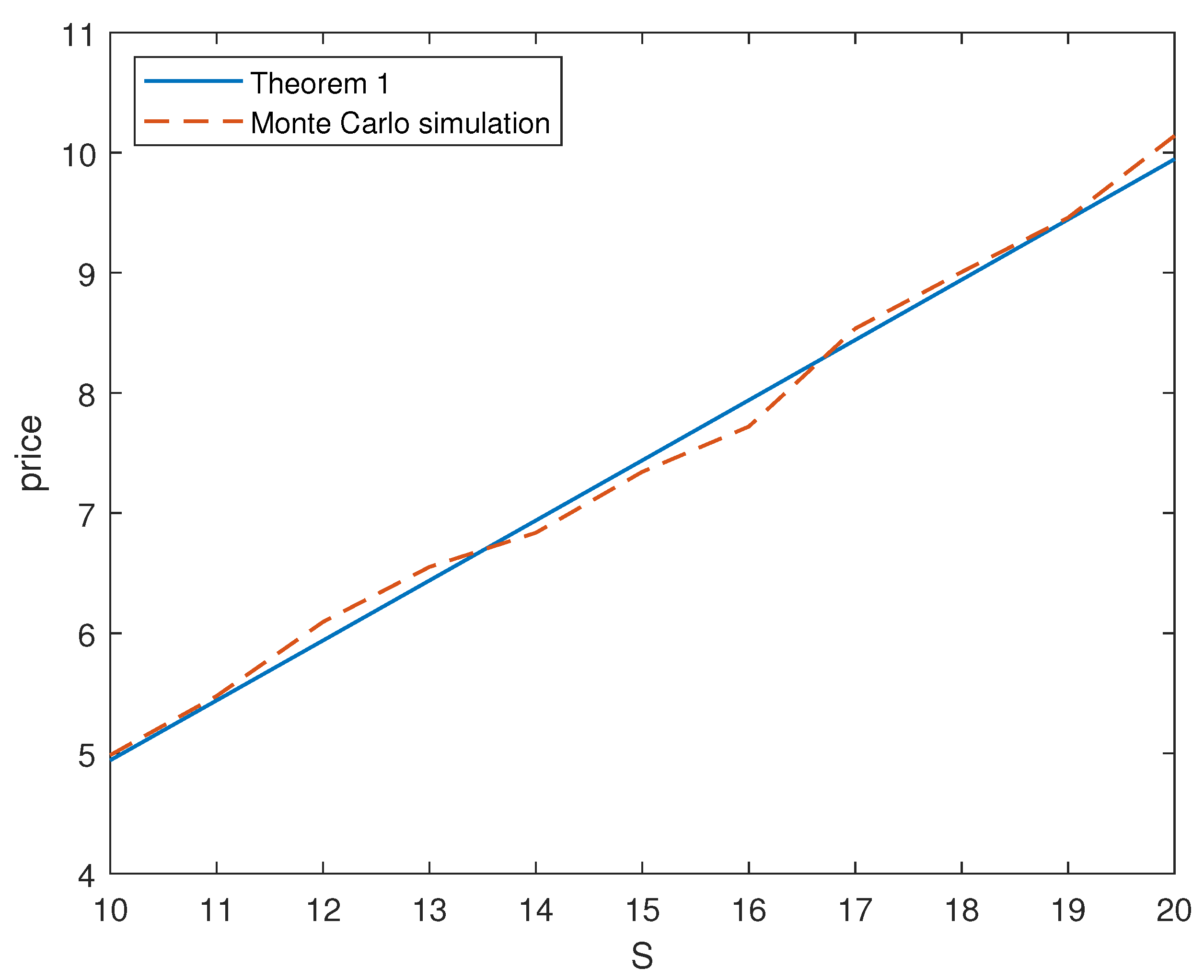
We simulate the prices of the binary option price under the MEJ-Heston–HW model according to Theorem 1 and the Monte Carlo method, which is shown in Figure 1. In Monte Carlo simulations, the parameters of the underlying asset are chosen as above, the number of simulations is 100,000, and the number of steps is set to 256. It can be seen from Figure 1 that the price trend simulated according to the formula of Theorem 1 and Monte Carlo method are consistent.

The percentage error of the ANOC price between Monte Carlo and Theorem 1 is shown in

Table 1. ANOC Price: Monte Carlo and Theorem 1 solution results for the MEJ-Heston–HW model.

S	Monte Carlo	Theorem 1	PE (%)
10	4.9855	4.9422	0.8685%
11	5.4779	5.4406	0.6809%
12	6.0942	5.9395	2.5385%
13	6.5517	6.4389	1.7212%
14	6.8364	6.9387	−1.4964%
15	7.3436	7.4389	−1.2977%
16	7.7197	7.9395	−2.8472%
17	8.5355	8.4404	0.1142%
18	9.0062	8.9417	0.7162%
19	9.4584	9.4433	0.1596%
20	10.1397	9.9452	1.9182%

. This indicates that the gap between the two methods is relatively small, which suggests that the pricing formula in this article is accurate and valid.

The binary option price under the MEJ-Heston–HW model is compared with the binary option price under the DEJ-Heston–HW and Heston–HW models. The exponent parameters of the DEJ-Heston–HW model are set to 50 and 40, and the Heston–HW models are obtained by removing the jump term from the MEJ-Heston–HW models; other parameters in the DEJ-Heston–HW and Heston–HW model are the same as in the MEJ-Heston–HW model. MATLAB(R2018b) is used to draw the price trend chart of the binary option that changes with the underlying asset (see Figure 2). We can see from the figure that the price of the option increases with an increase in the underlying asset. The binary option price of MEJ-Heston–HW model in this paper is always higher than the price of DEJ-Heston–HW model and Heston–HW model. The mixed exponential jump model is an extension of the double exponential jump model. Compared with the DEJ-Heston–HW model, the price volatility of the underlying asset described by the MEJ-Heston–HW model is larger, i.e., the risk of investment is higher, so the price of the binary option is higher.

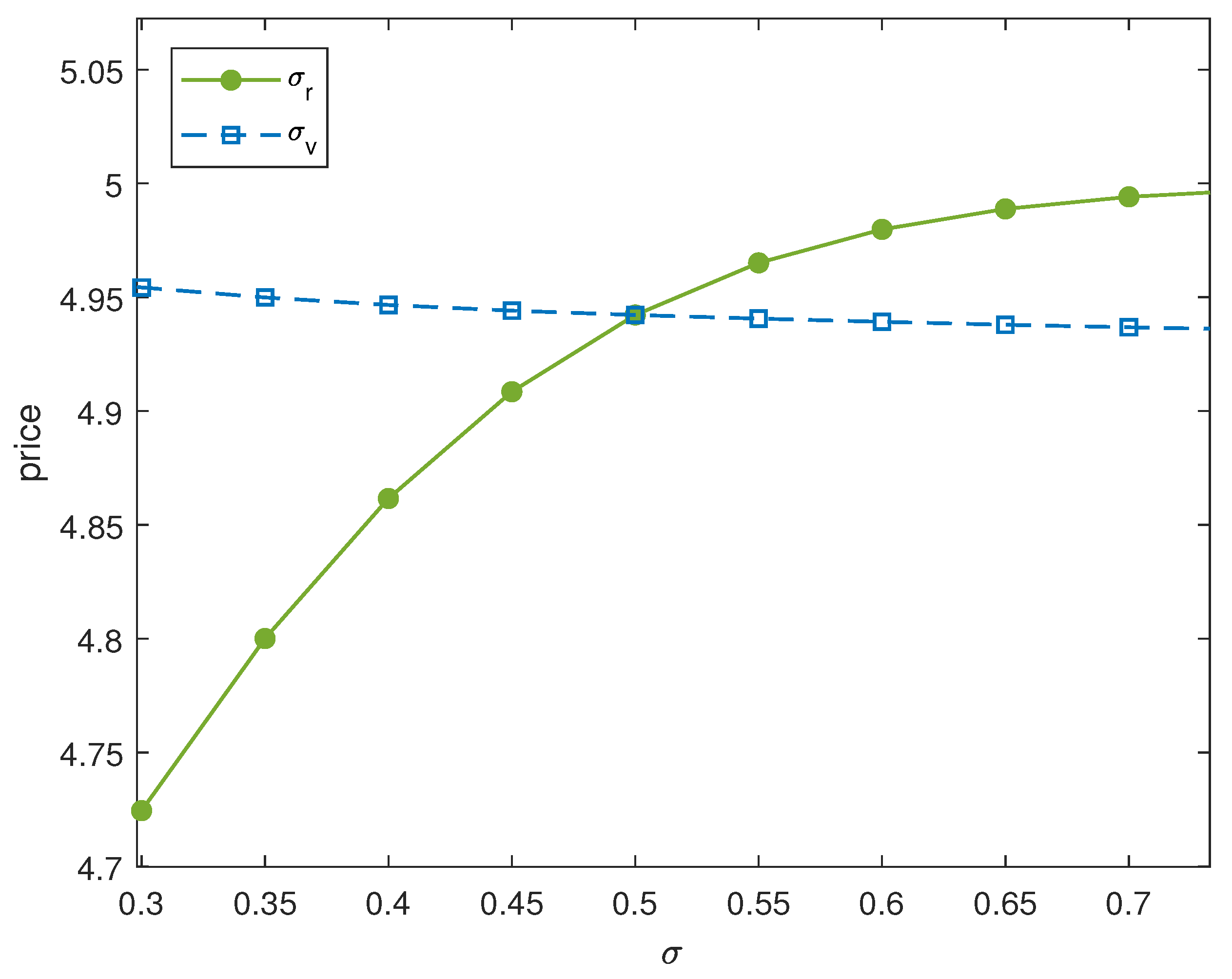
The effects of some parameters in the model on the price of the binary option are shown below. Figure 3 shows the relation between the price of binary options and the volatilities ${\sigma }_r$, ${\sigma }_v$. It can be observed from Figure 3 that the volatility term in the stochastic volatility model has a more positive impact on the option price, while the volatility term in the stochastic interest rate model is relatively stable for the option price.

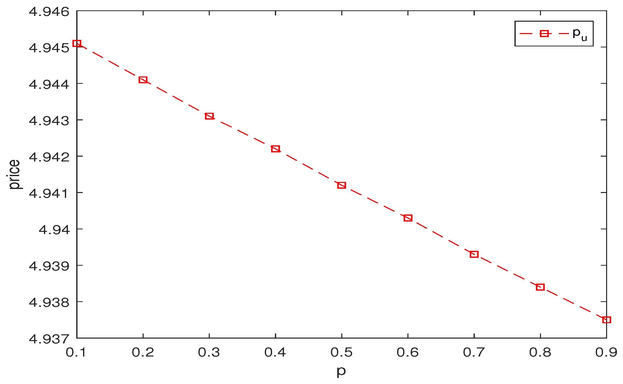
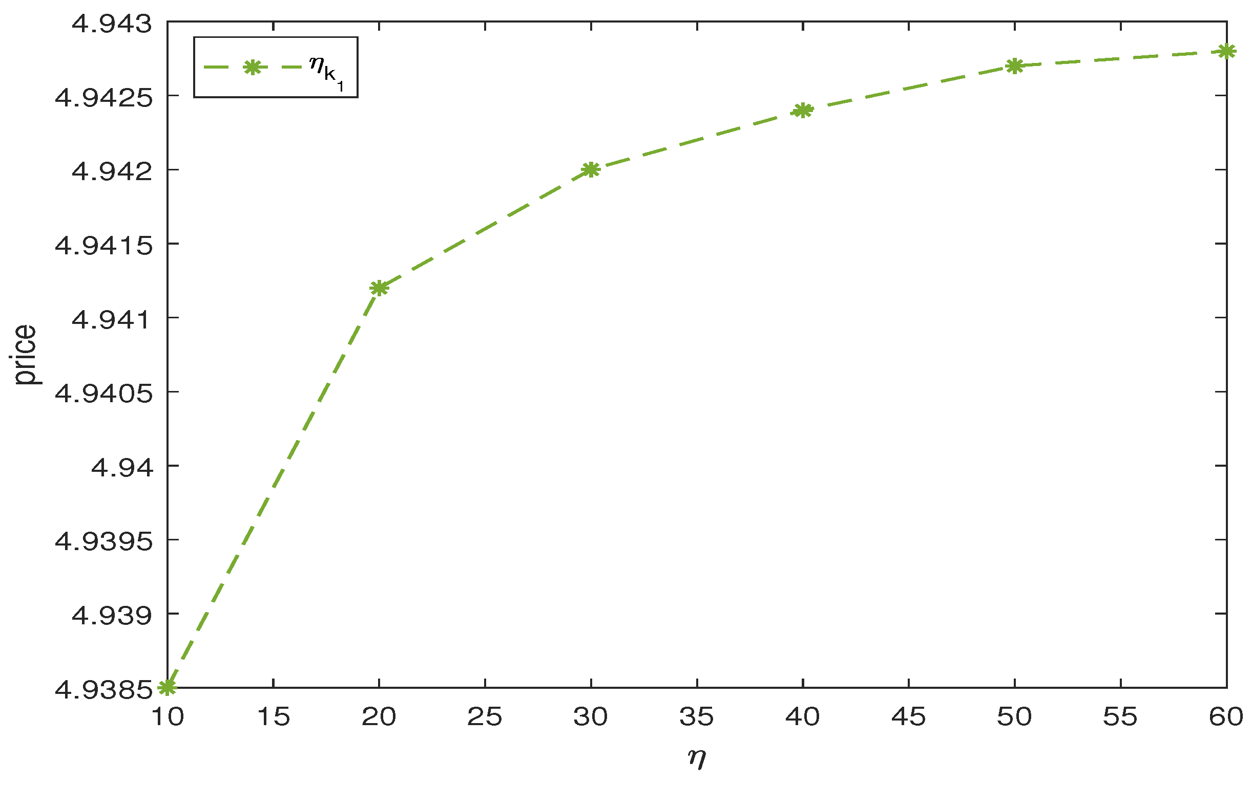
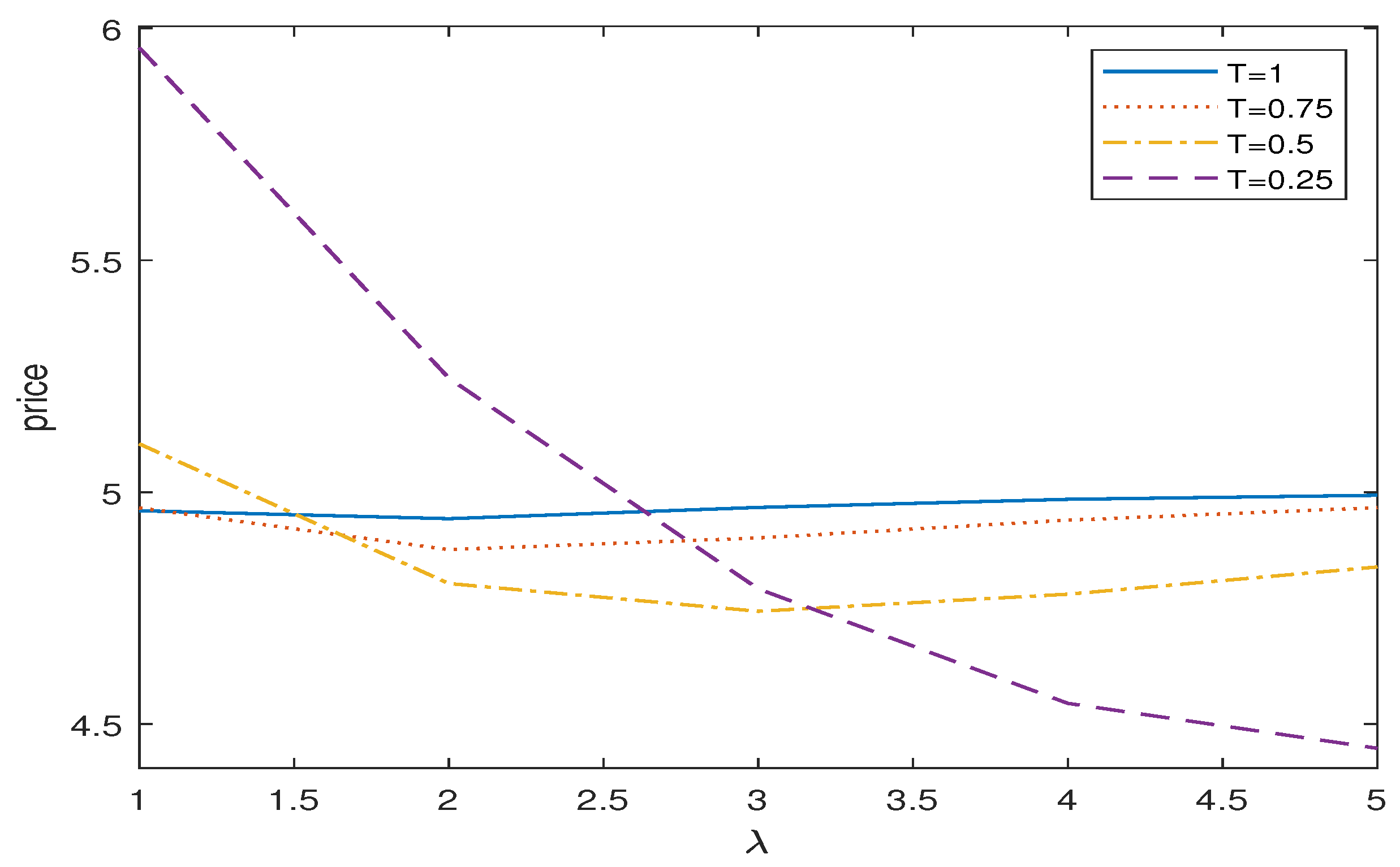
Figure 4, Figure 5, Figure 6 and Figure 7 give the relation between the binary call option price and the positive jump probability $p_u$, the exponential parameter ${\eta }_{k_1}$, ${\theta }_{k_1}$, and the jump intensity $\lambda$ in the jump-diffusion term of the MEJ-Heston–HW model, and it can be observed that the binary call option price is negatively correlated with the upward jump probability $p_u$ in Figure 4. Figure 5 and Figure 6 show that the binary call option price increases with an increase in the index parameter ${\theta }_{k_1}$ in the positive jump, and decreases with an increase in the index parameter ${\eta }_{k_1}$ in the negative jump in the mixed index jump. Figure 7 shows that the price of binary option presents a negative correlation trend with the increase in jump intensity, and the price fluctuation of binary options tends to be stable with the increase in expiration date. Therefore, when trading binary options, investors should not only pay attention to the systemic risk in a stable state, but also pay attention to the jump risk caused by the stock price due to unexpected events, so as to carry out effective financial risk management.

5. Conclusions

This paper studies the pricing problem of binary options under the assumption that the underlying asset price follows the MEJ-Heston–HW model. The pricing formula of the call binary option under the MEJ-Heston–HW model is obtained by using the Fourier transform. The binary option prices of MEJ-Heston–HW model, DEJ-Heston–HW model, and Heston–HW model are compared by numerical simulation, and the influence of parameters in MEJ-Heston–HW model on the binary option prices is studied and discussed. The results show that these parameters have an important impact on option price.

For future research, we can consider the pricing of other exotic options under the MEJ-Heston–HW model, such as vulnerable binary options and so on.

References

1. Black, F.; Scholes, M. The pricing of options and corporate liabilities. J. Political Econ. 1973, 81, 637–654. [Google Scholar] [CrossRef]
2. Rubinstein, M.; Reiner, E. Unscrambling the binary code. J. Risk 1991, 4, 75–83. [Google Scholar]
3. Chen, R.D.; Zhou, H.X.; Yu, L.A.; Jin, C.L.; Zhang, S.N. An efficient method for pricing foreign currency options. J. Int. Financ. Mark. Inst. Money 2021, 2, 101295. [Google Scholar] [CrossRef]
4. Heston, S.L. A closed-form solution for options with stochastic volatility with applications to bond and currency options. J. Rev. Financ. Stud. 1993, 6, 327–343. [Google Scholar] [CrossRef]
5. Fonseca, J.D.; Grasselli, M.; Tebaldi, C. A multifactor volatility heston model. J. Quant. Financ. 2008, 8, 591–604. [Google Scholar] [CrossRef]
6. He, X.J.; Zhu, S.P. An analytical approximation formula for European option pricing under a newstochastic volatility model with regime-switching. J. Econ. Dyn. Control 2016, 71, 77–85. [Google Scholar] [CrossRef]
7. Vasicek, O.A. An equilibrium characterization of the term structure. J. Financ. Econ. 1977, 5, 177–188. [Google Scholar] [CrossRef]
8. Cox, J.; Ingersoll, J.; Stephen, R. An intertemporal general equilibrium model of asset prices and a theory of the term structure of interest rates. Econometrica 1985, 52, 363–407. [Google Scholar] [CrossRef]
9. Hull, J.; Alan, W. Pricing interest rate derivative securities. J. Rev. Financ. Stud. 1990, 3, 573–592. [Google Scholar] [CrossRef]
10. Merton, R.C. Option pricing when underlying stock returns are discontinuous. J. Financ. Econ. 1976, 3, 125–144. [Google Scholar] [CrossRef]
11. Kou, S.G. A jump-diffusion model for option pricing. J. Manag. Sci. 2002, 48, 1086–1101. [Google Scholar] [CrossRef]
12. Cai, N.; Kou, S.G. Option pricing under a mixed-exponential jump diffusion model. J. Manag. Sci. 2011, 57, 2067–2081. [Google Scholar] [CrossRef]
13. Kolková, A.; Lenertová, L. Binary options as a modern fenomenon of financial business. Int. J. Entrep. Behav. R. 2016, 1, 52–59. [Google Scholar]
14. Liu, G.X.; Zhu, Q.X.; Yan, Z.W. The martingale approach for vulnerable binary option pricing under stochastic interest rate. Cogent. Math. 2017, 4, 1340073. [Google Scholar] [CrossRef]
15. Thavaneswaran, A.; Appadoo, S.S.; Frank, J. Binary Option Pricing Using Fuzzy Numbers. J. Appl. Math. Lett. 2013, 26, 65–72. [Google Scholar] [CrossRef]
16. He, X.J.; Chen, W.T. A Monte-Carlo based approach for pricing credit default swaps with regime switching. Comput. Math. Appl. 2018, 7, 1758–1766. [Google Scholar] [CrossRef]
17. Gao, M. The British binary options. J. Math. Financ. 2019, 9, 747–762. [Google Scholar] [CrossRef]
18. Qin, X.; Lin, X.; Shang, Q. Fuzzy pricing of binary option based on the long memory property of financial markets. J. Intell. Fuzzy. Syst. 2020, 4, 4889–4900. [Google Scholar] [CrossRef]
19. Nikita, R. On barrier binary options in the telegraph-like financial market model. Computation 2022, 9, 163. [Google Scholar] [CrossRef]
20. Yang, M.; Gao, Y. Pricing formulas of binary options in uncertain financial markets. AIMS Math. 2023, 8, 23336–23351. [Google Scholar] [CrossRef]
21. Klebaner, F.C. Introduction to Stochastic Calculus with Applications; Imperial College Press: London, UK, 2012; pp. 91–120. [Google Scholar]
22. Shreve, S.E. Stochastic Calculus for Finance II; Springer: New York, NY, USA, 2007; pp. 234–237. [Google Scholar]
23. Deng, G.H. Pricing European option in a double exponential jump-diffusion model with two market structure risks and its comparisons. J. Appl. Math. Ser. B 2007, 22, 127–137. [Google Scholar] [CrossRef]
Figure 1. Monte Carlo simulation and numerical simulation of Theorem 1.
Mathematics 12 03233 g001
Figure 2. Comparison of binary call option prices under MEJ-Heston–HW model with the Heston–HW model and the DEJ-Heston–HW model.
Mathematics 12 03233 g002
Figure 3. The relation between binary call option price and volatility σ r , σ v under the MEJ-Heston–HW model.
Mathematics 12 03233 g003
Figure 4. The effect of the upward jump probability P u on the price of the binary call option.
Mathematics 12 03233 g004
Figure 5. The effect of the index parameter θ k 1 on the price of the binary call option.
Mathematics 12 03233 g005
Figure 6. The effect of the index parameter η k 1 on the price of the binary call option.
Mathematics 12 03233 g006
Figure 7. T takes different values of binary call option prices vary with λ .
Mathematics 12 03233 g007