
A Graph-Refinement Algorithm to Minimize Squared Delivery Delays Using Parcel Robots


Abstract
1. Introduction
- We present and model a real-world problem, the TBDRP, as a MIQP. This model accounts for battery consumption, soft time-window constraints and supports partial recharging.
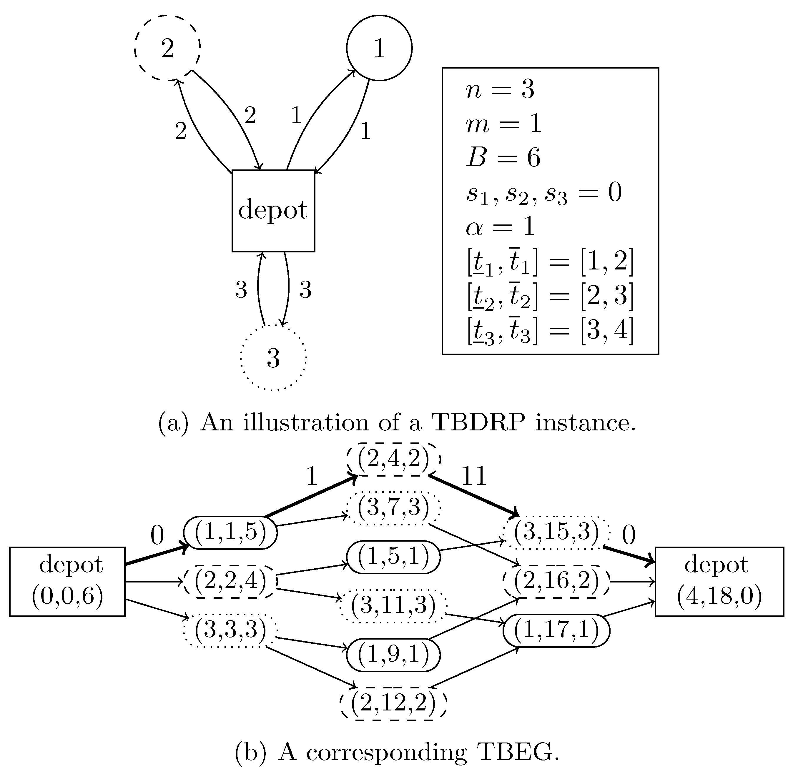
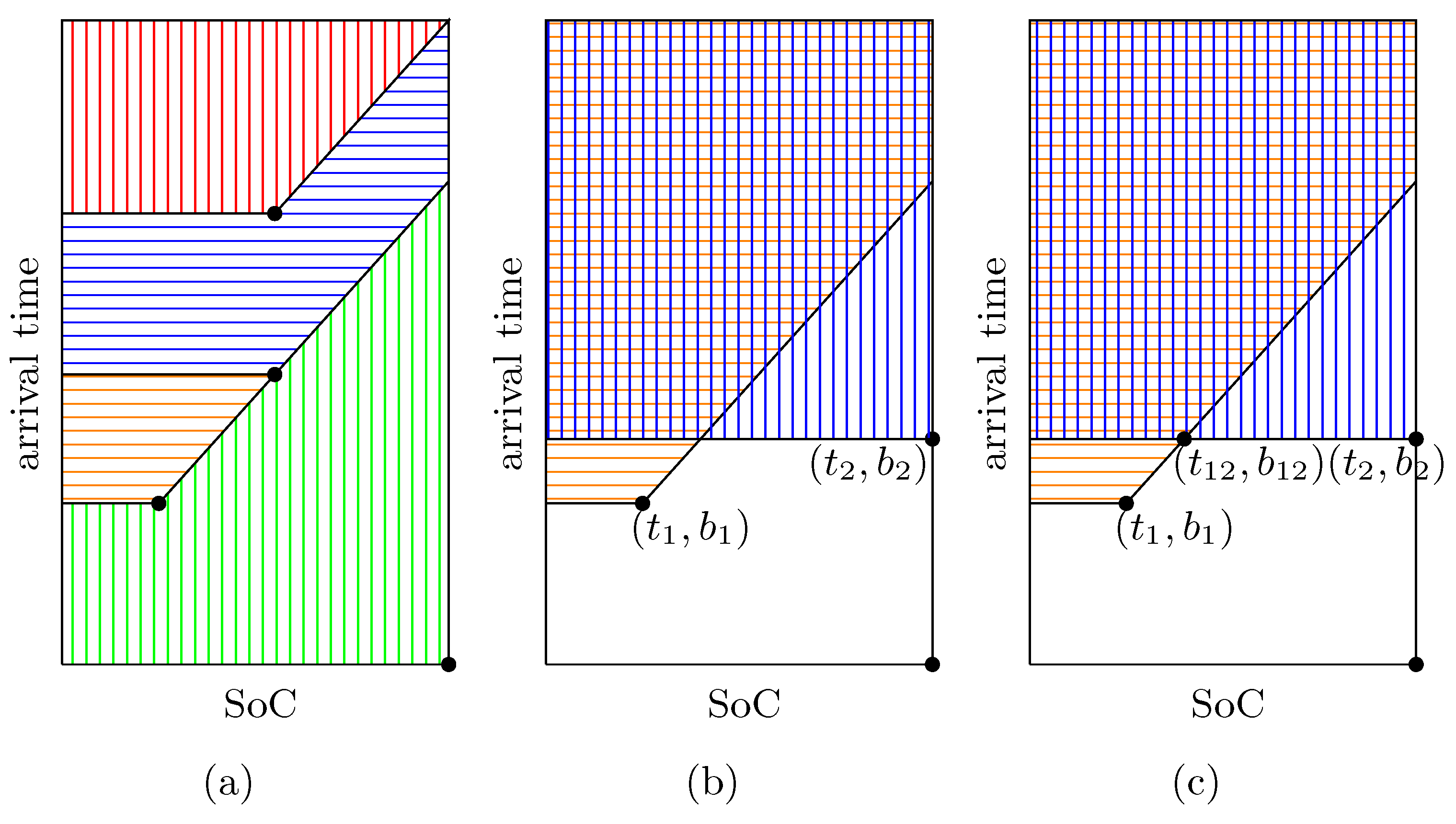
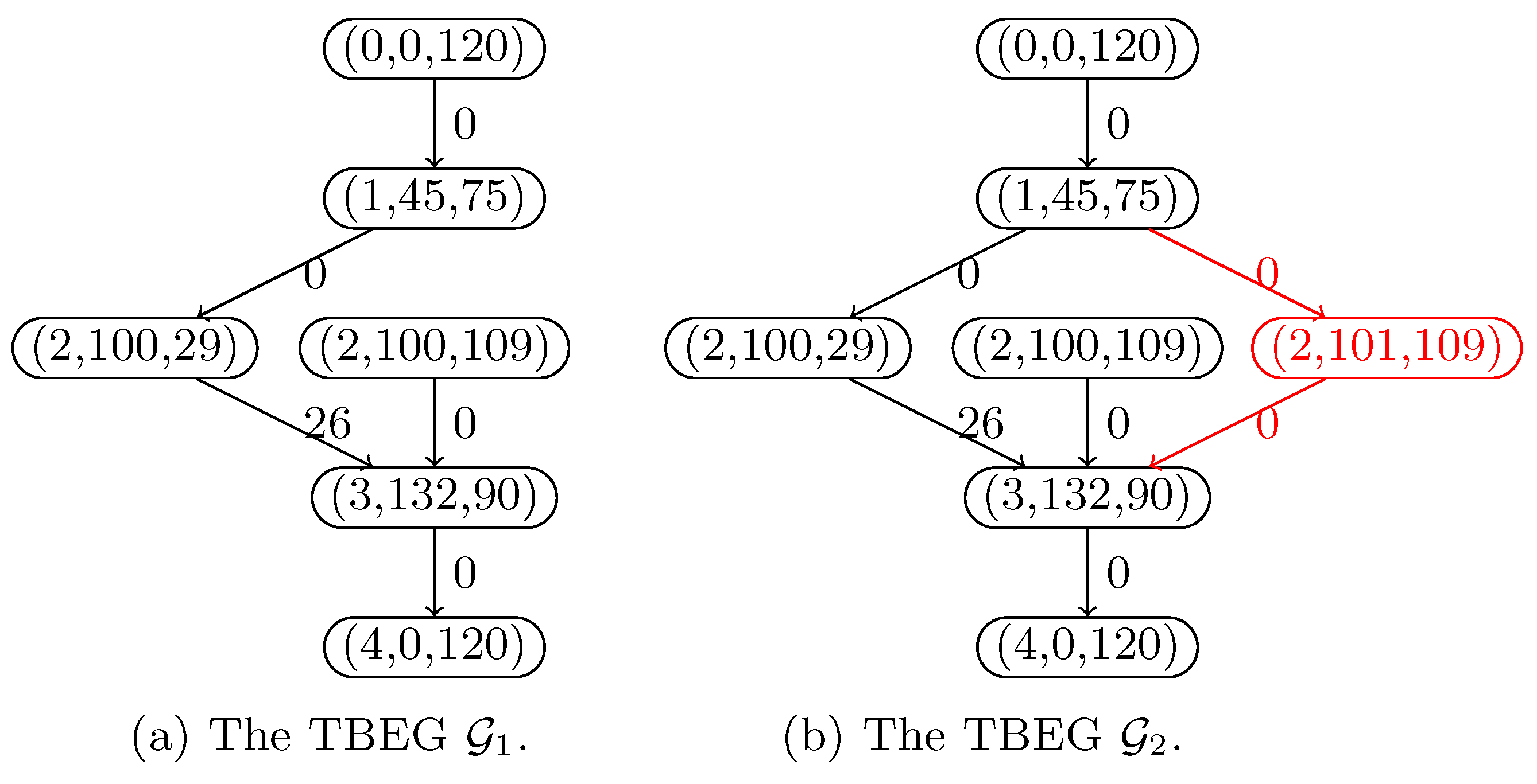
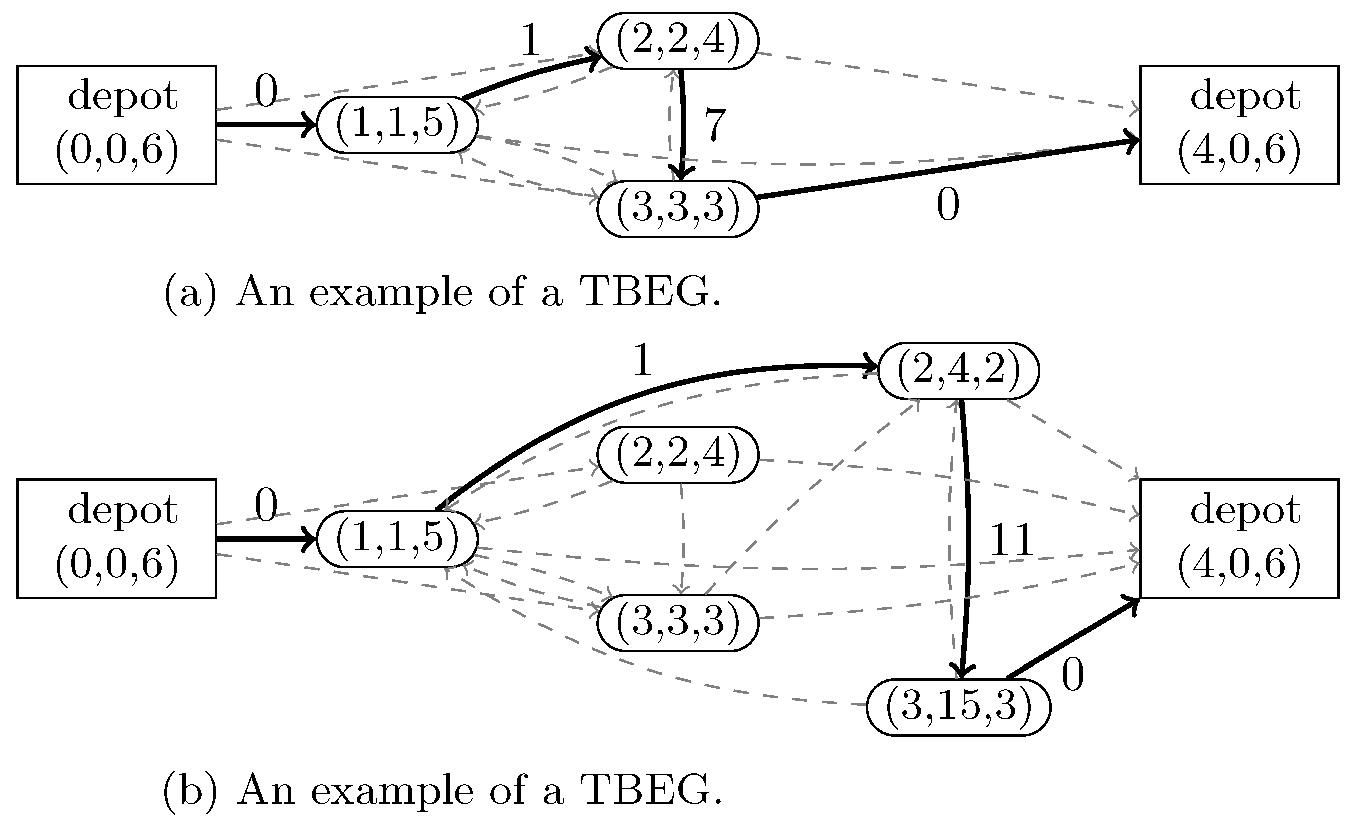
- We propose an alternative formulation using two-dimensional layered graphs and demonstrate that aggregated layered graphs can be employed to find relaxations of the TBDRP.
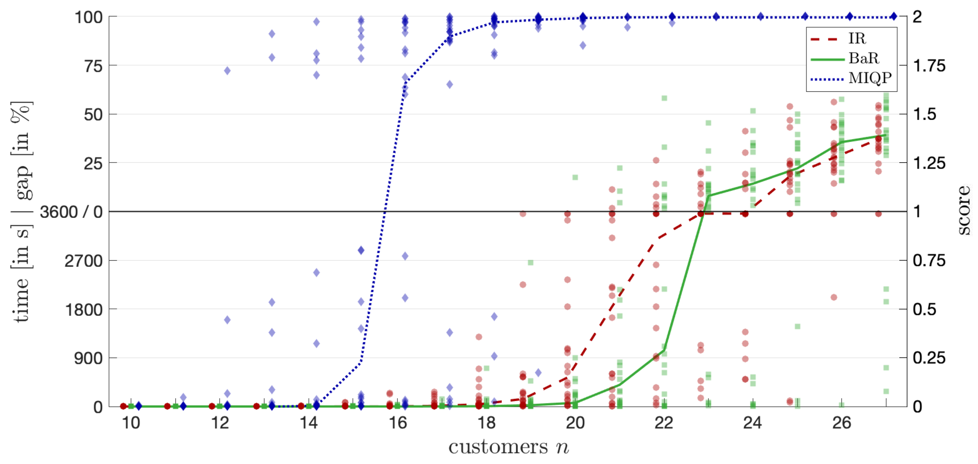
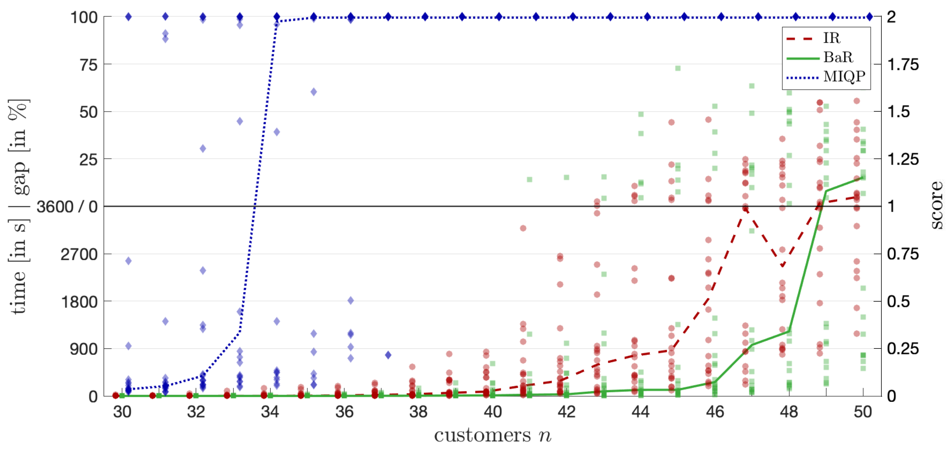
- We develop two algorithms based on these relaxations and show through computational experiments that they outperform direct approaches to solving the MIQP formulation using state-of-the-art solvers.
2. Literature Review
3. Problem Description and Mathematical Formulation
3.1. Exact Mixed-Integer Formulations
3.2. The Time- and Battery-Expanded Formulation
| Algorithm 1: |
 |
| Algorithm 2: |
1 Input: A node representative of some location and another location j, such that ; 2 ; (forced charging time) 3 ; (forced wait time) 4 ; (time at depot) 5 ; (arrival time at j) 6 ; (SoC at j) 7 Output: A node representative of j; |
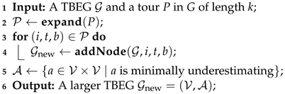
| Algorithm 3: expand |
 |
4. Relaxations of the Time- and Battery-Expanded Formulation
| Algorithm 4: |
1 Input: Node representatives and of some location ; 2 ; 3 ; 4 ; 5 ; 6 Output: A node representative of j; |
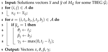
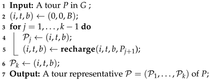
| Algorithm 5: |
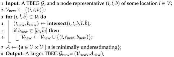 |
| Algorithm 6: |
 |
5. Refinement Algorithms
| Algorithm 7: Iterative Refinement Algorithm |
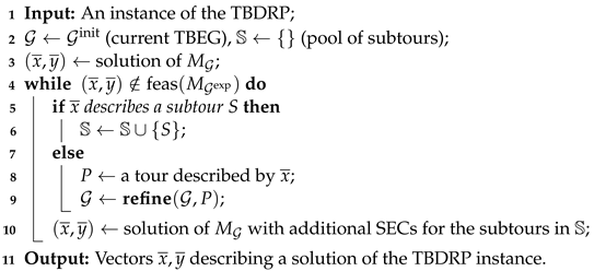 |
| Algorithm 8: Branch and Refine |
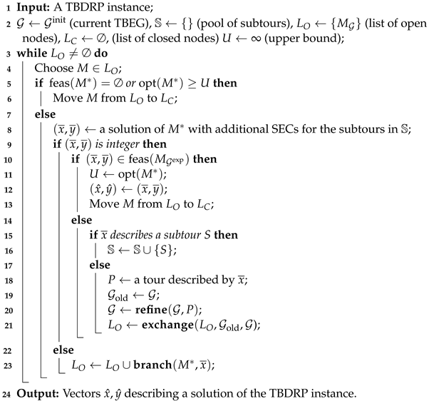 |
6. Computational Experiments and Implementation Details
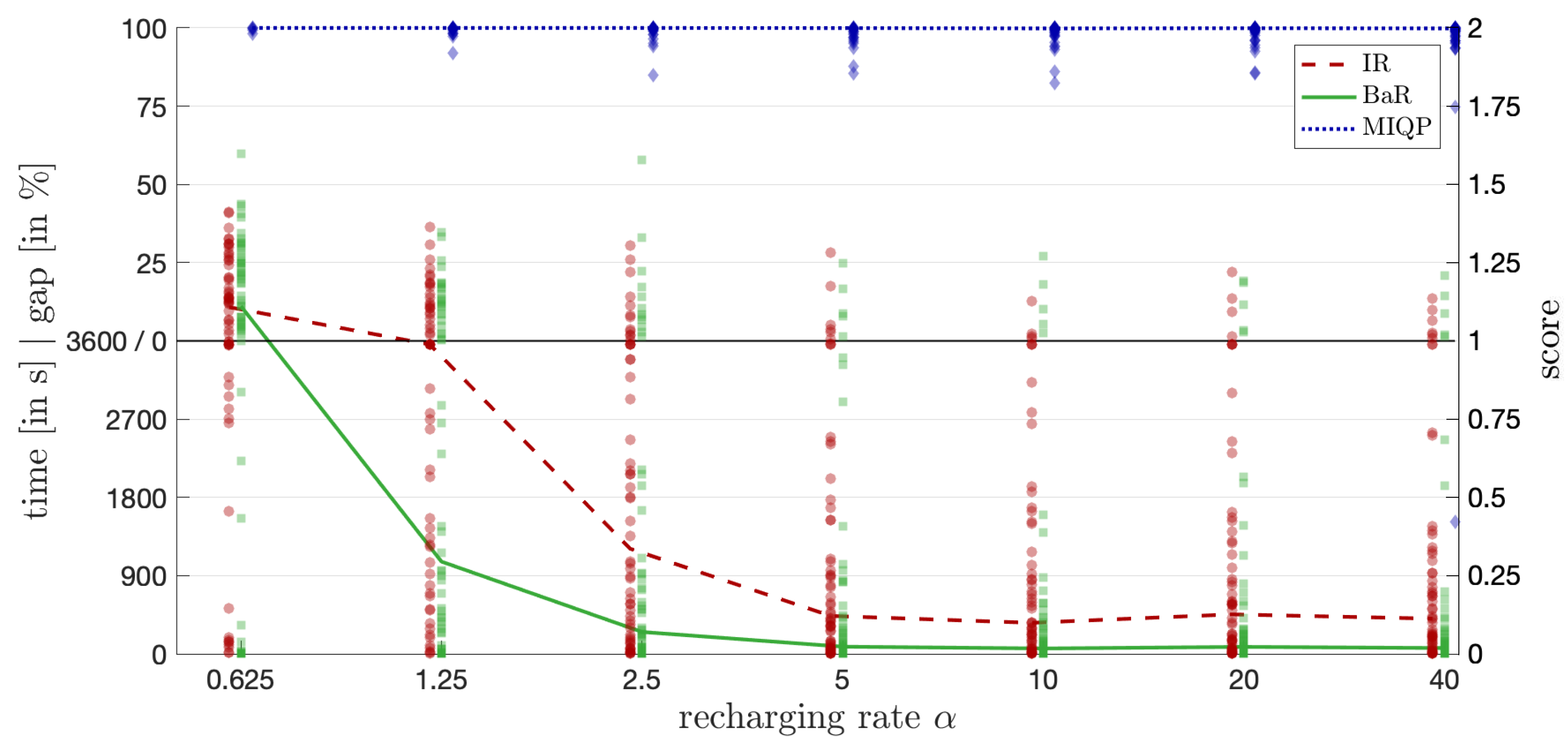
- Computation Time Score (): For instances solved to proven optimality within the time limit s, we compute a normalized computation time score:where t is the computation time in seconds. This maps the computation time linearly onto the interval , with lower values indicating better performance.
- Optimality Gap Score (): For instances not solved to proven optimality within the time limit, we record the optimality gap at termination:where and are the best upper and lower bounds found by the algorithm, respectively. We normalize the gap to a score between 0 and 1:with higher values indicating a larger gap and thus poorer performance.
- Total Score (): The total score for each instance is the sum of the computation time score and the optimality gap score:This results in a total score s ranging from 0 (best possible performance) to 2 (worst possible performance), effectively combining both time and solution quality into a single metric.
7. Conclusions and Future Work
Author Contributions
Funding
Data Availability Statement
Acknowledgments
Conflicts of Interest
References
- Statista Digital Market Outlook. Ecommerce Report 2022. 2022. Available online: https://www.statista.com/study/42335/ecommerce-report/ (accessed on 7 October 2024).
- Pitney Bowes Inc. Pitney Bowes Parcel Shipping Index Reports Continued Growth as Global Parcel Volume Exceeds 100 Billion for First Time Ever. 2020. Available online: https://www.businesswire.com/news/home/20180828005237/en/ (accessed on 7 October 2024).
- Heinemann, G. Der Neue Online-Handel; Springer Fachmedien: Wiesbaden, Germany, 2018. [Google Scholar]
- Kreuz, F.; Clausen, U. Einsatzfelder von eLastenrädern im Städtischen Wirtschaftsverkehr; Springer Fachmedien: Wiesbaden, Germany, 2017; pp. 323–333. [Google Scholar]
- Boysen, N.; Fedtke, S.; Schwerdfeger, S. Last-mile delivery concepts: A survey from an operational research perspective. OR Spectr. 2020, 43, 1–58. [Google Scholar] [CrossRef]
- Engesser, V.; Rombaut, E.; Vanhaverbeke, L.; Lebeau, P. Autonomous Delivery Solutions for Last-Mile Logistics Operations: A Literature Review and Research Agenda. Sustainability 2023, 15, 2774. [Google Scholar] [CrossRef]
- Speranza, M.G. Trends in transportation and logistics. Eur. J. Oper. Res. 2018, 264, 830–836. [Google Scholar] [CrossRef]
- Boysen, N.; Schwerdfeger, S.; Weidinger, F. Scheduling last-mile deliveries with truck-based autonomous robots. Eur. J. Oper. Res. 2018, 271, 1085–1099. [Google Scholar] [CrossRef]
- Ostermeier, M.; Heimfarth, A.; Hübner, A. Cost-optimal truck-and-robot routing for last-mile delivery. Networks 2022, 79, 364–389. [Google Scholar] [CrossRef]
- Poeting, M.; Schaudt, S.; Clausen, U. Simulation of an Optimized Last-Mile Parcel Delivery Network Involving Delivery Robots. In Advances in Production, Logistics, and Traffic—Proceedings of the 4th Interdisciplinary Conference on Production Logistics and Traffic 2019; Clausen, U., Langkau, S., Kreuz, F., Eds.; Lecture Notes in Logistics; Springer Nature Switzerland AG: Cham, Switzerland, 2019; pp. 1–19. [Google Scholar]
- Poeting, M.; Schaudt, S.; Clausen, U. A comprehensive case study in last-mile delivery concepts for parcel robots. In Proceedings of the 2019 Winter Simulation Conference (WSC), National Harbor, MD, USA, 8–11 December 2019. [Google Scholar]
- Sonneberg, M.-O.; Leyerer, M.; Kleinschmidt, A.; Knigge, F.; Breitner, M.H. Autonomous unmanned ground vehicles for urban logistics: Optimization of last mile delivery operations. In Proceedings of the 52nd Hawaii International Conference on System Sciences, Hawaii International Conference on System Sciences, Hawaii, HI, USA, 8–11 January 2019. [Google Scholar]
- Maio, A.D.; Ghiani, G.; Laganá, D.; Manni, E. Sustainable last-mile distribution with autonomous delivery robots and public transportation. Transp. Res. Part C Emerg. Technol. 2024, 163, 104615. [Google Scholar] [CrossRef]
- Viloria, D.R.; Solano-Charris, E.L.; Muñoz-Villamizar, A.; Montoya-Torres, J.R. Unmanned aerial vehicles/drones in vehicle routing problems: A literature review. Int. Trans. Oper. Res. 2021, 28, 1626–1657. [Google Scholar] [CrossRef]
- Boysen, N.; Briskorn, D.; Fedtke, S.; Schwerdfeger, S. Drone delivery from trucks: Drone scheduling for given truck routes. Networks 2018, 72, 506–527. [Google Scholar] [CrossRef]
- Poikonen, S.; Wang, X.; Golden, B. The vehicle routing problem with drones: Extended models and connections. Networks 2017, 70, 34–43. [Google Scholar] [CrossRef]
- Wang, Z.; Sheu, J.-B. Vehicle routing problem with drones. Transp. Res. Part B Methodol. 2019, 122, 350–364. [Google Scholar] [CrossRef]
- Erdelić, T.; Carić, T. A survey on the electric vehicle routing problem: Variants and solution approaches. J. Adv. Transp. 2019, 2019, 5075671. [Google Scholar] [CrossRef]
- Schneider, M.; Stenger, A.; Goeke, D. The electric vehicle-routing problem with time windows and recharging stations. Transp. Sci. 2014, 48, 500–520. [Google Scholar] [CrossRef]
- Keskin, M.; Çatay, B. Partial recharge strategies for the electric vehicle routing problem with time windows. Transp. Res. Part C Emerg. Technol. 2016, 65, 111–127. [Google Scholar] [CrossRef]
- Desaulniers, G.; Errico, F.; Irnich, S.; Schneider, M. Exact algorithms for electric vehicle-routing problems with time windows. Oper. Res. 2016, 64, 1388–1405. [Google Scholar] [CrossRef]
- Gouveia, L.; Leitner, M.; Ruthmair, M. Layered graph approaches for combinatorial optimization problems. Comput. Oper. Res. 2019, 102, 22–38. [Google Scholar] [CrossRef]
- Boland, N.L.; Savelsbergh, M.W. Perspectives on integer programming for time-dependent models. Top 2019, 27, 147–173. [Google Scholar] [CrossRef]
- Boland, N.; Hewitt, M.; Marshall, L.; Savelsbergh, M. The continuous-time service network design problem. Oper. Res. 2017, 65, 1303–1321. [Google Scholar] [CrossRef]
- Vu, D.M.; Hewitt, M.; Boland, N.; Savelsbergh, M. Dynamic discretization discovery for solving the time-dependent traveling salesman problem with time windows. Transp. Sci. 2020, 54, 703–720. [Google Scholar] [CrossRef]
- He, E.; Boland, N.; Nemhauser, G.; Savelsbergh, M. A dynamic discretization discovery algorithm for the minimum duration time-dependent shortest path problem. In International Conference on the Integration of Constraint Programming, Artificial Intelligence, and Operations Research; Springer: Berlin/Heidelberg, Germany, 2018; pp. 289–297. [Google Scholar]
- Riedler, M.; Ruthmair, M.; Raidl, G.R. Strategies for iteratively refining layered graph models. In International Workshop on Hybrid Metaheuristics; Springer: Berlin/Heidelberg, Germany, 2019; pp. 46–62. [Google Scholar]
- Gnegel, F.; Fügenschuh, A. An iterative graph expansion approach for the scheduling and routing of airplanes. Comput. Oper. Res. 2020, 114, 104832. [Google Scholar] [CrossRef]
- Bärmann, A.; Liers, F.; Martin, A.; Merkert, M.; Thurner, C.; Weninger, D. Solving network design problems via iterative aggregation. Math. Program. Comput. 2015, 7, 189–217. [Google Scholar] [CrossRef]
- Clautiaux, F.; Hanafi, S.; Macedo, R.; Voge, M.-E.; Alves, C. Iterative aggregation and disaggregation algorithm for pseudo-polynomial network flow models with side constraints. Eur. J. Oper. Res. 2017, 258, 467–477. [Google Scholar] [CrossRef]
- Marra, F.; Yang, G.Y.; Træholt, C.; Larsen, E.; Rasmussen, C.N.; You, S. Demand profile study of battery electric vehicle under different charging options. In Proceedings of the 2012 IEEE Power and Energy Society General Meeting, San Diego, CA, USA, 22–26 July 2012; pp. 1–7. [Google Scholar]
- Solomon, M.M. Algorithms for the vehicle routing and scheduling problems with time window constraints. Oper. Res. 1987, 35, 254–265. [Google Scholar] [CrossRef]


| Variable | Description |
|---|---|
| indicator if location i precedes location j for | |
| start of the service at location | |
| SoC at location | |
| delay at location | |
| m | number of vehicles |
| n | number of customers |
| service time at customer | |
| travel time from the depot to customer | |
| traveling plus service time for | |
| battery consumption for | |
| T | time horizon |
| time window of location | |
| B | battery capacity |
| battery window of location | |
| recharging rate |
| Customer | Time Window | Depot Distance | Battery Interval |
|---|---|---|---|
| 1 | 45 | ||
| 2 | 11 | ||
| 3 | 30 |
Disclaimer/Publisher’s Note: The statements, opinions and data contained in all publications are solely those of the individual author(s) and contributor(s) and not of MDPI and/or the editor(s). MDPI and/or the editor(s) disclaim responsibility for any injury to people or property resulting from any ideas, methods, instructions or products referred to in the content. |
© 2024 by the authors. Licensee MDPI, Basel, Switzerland. This article is an open access article distributed under the terms and conditions of the Creative Commons Attribution (CC BY) license (https://creativecommons.org/licenses/by/4.0/).
Share and Cite
Gnegel, F.; Schaudt, S.; Clausen, U.; Fügenschuh, A. A Graph-Refinement Algorithm to Minimize Squared Delivery Delays Using Parcel Robots. Mathematics 2024, 12, 3201. https://doi.org/10.3390/math12203201
Gnegel F, Schaudt S, Clausen U, Fügenschuh A. A Graph-Refinement Algorithm to Minimize Squared Delivery Delays Using Parcel Robots. Mathematics. 2024; 12(20):3201. https://doi.org/10.3390/math12203201
Chicago/Turabian StyleGnegel, Fabian, Stefan Schaudt, Uwe Clausen, and Armin Fügenschuh. 2024. "A Graph-Refinement Algorithm to Minimize Squared Delivery Delays Using Parcel Robots" Mathematics 12, no. 20: 3201. https://doi.org/10.3390/math12203201
APA StyleGnegel, F., Schaudt, S., Clausen, U., & Fügenschuh, A. (2024). A Graph-Refinement Algorithm to Minimize Squared Delivery Delays Using Parcel Robots. Mathematics, 12(20), 3201. https://doi.org/10.3390/math12203201