On the Number of Customer Classes in a Single-Period Inventory System

Abstract

A common practice in inventory systems with several customers requiring differentiated service levels is to group them into two or three classes, where a customer class is a group of customers with the same preset service level in terms of product availability. However, there is no evidence that grouping customers into two or three classes is optimal in terms of the ordering policy parameters. This paper studies the effect of the number of customer classes on the inventory level of a single-period inventory system with stochastic demand and individual service-level requirements from multiple customer classes. Using a Sample Average Approximation approach, we formulate computationally tractable multi-class service level models, under responsive and anticipative priority policies in cases of shortage, as mixed integer linear problems (MIPs). The effect of the number of classes on the inventory level is determined using a round-up aggregation scheme; i.e., given a sufficiently large initial number of classes, it is reduced by adding the lower service level classes to the next higher class. We analytically characterize the optimal inventory level under responsive and anticipative priority policies as a function of the initial number of classes and the number of classes grouped based on the round-up aggregation scheme. Under a responsive priority policy, we show that there is an optimal number of classes, while under an anticipative priority policy, the optimal number of classes is equal to the initial number of classes. The effect of free-riders resulting from the round-up aggregation scheme on the optimal inventory level is studied through numerical experiments.

1. Introduction

Research on inventory systems subject to multiple customer classes is based on the fact that, for the same product, demand may arise from different customer groups with varying requirements for delivery times or service levels regarding product availability. Although these inventory systems have been extensively studied, less attention has been focused on the single-period problem under stochastic demand and individual service-level requirements from multiple customer classes. This scenario is not unusual; we are talking about a relatively common situation, e.g., wholesalers supplying products to different customers in a retail market, and where the attention priority of each customer, as well as their demand, is different.

In these scenarios, a key challenge is to minimize the amount of products the wholesaler needs to meet customer demand, all while ensuring a specified service level. This is especially important in shortage situations. A common practice is to group customers into two or three customer classes, using Pareto or ABC classifications, respectively, where A-class represents priority customers who can demand high service levels. However, to the best of our knowledge, there is no evidence that grouping customers into two or three classes achieves inventory level minimization in a single-period inventory system with multiple customer classes. The complexity of this problem, arising when customers are grouped into more than three classes, has hindered research on the effect of the number of customer classes on inventory level in this type of inventory system.

In this paper, we consider a seasonal product wholesaler who serves several customer classes with different service level requirements in terms of product availability; the wholesaler is likely to face shortages because the purchase order is made before knowing the real demand of its different customer classes. Given this situation, the wholesaler has to make two decisions. The first one is the amount of products to purchase and the second decision involves determining how to allocate the available inventory when the purchased quantity is less than the total demand. Two types of priority policies can be identified in the case of shortage, (i) responsive priority policies, where the order in which customer classes are going to be served (priority list) is defined using the realized demand information, and (ii) anticipative priority policies, where a priority list is defined before demand realization. The simplest responsive policy is the greedy allocation priority policy (GP policy), where customers are served in ascending order according to the demand realization, while the simplest anticipative policy is the fixed-list allocation priority policy (FLP policy), where customers are served in descending order based on the preset service level of each customer class.

The objective of this paper is to determine the effect of the number of customer classes on the inventory level of a single-period inventory system with stochastic demand and individual service level requirements from multiple customer classes. The research questions we consider in this paper are as follows: (i) How does the number of customer classes affect the inventory level under different priority policies? (ii) What is the optimal number of customer classes under different demand configurations? and (iii) What priority policy performs better under different demand configurations?

To address this issue, both priority policies mentioned above, GP and FLP, are used, and the service level, considered to ensure product availability for each customer class, is measured by the probability of satisfying the entire demand for each class, namely, the $\alpha$ service-level. For each priority policy, we formulate a multi-customer class service-level constraint (SLC) problem under the $\alpha$ service level as a chance-constrained stochastic programming model. These $\alpha$-SLC problems are difficult to solve since they imply leading with convolutions and multiple integrals when customers are grouped into more than three classes, which limits the study of how the number of classes affects the inventory level. An efficient way to deal with chance constraints is to utilize the Sample Average Approximation (SAA) approach. The basic idea of SAA in problems where chance constraints are involved is to replace the theoretical distribution function by the empirical distribution obtained from random sampling. Thus, we show how to formulate the multi-customer class SLC models with chance constraints as mixed integer linear problems (MIPs) using a sample-based approach (SAA models), and taking advantage of the SAA method, we obtain a feasible solution with guaranteed quality in terms of its optimality gap. Then, assuming knowledge of the number of initial classes ($n>>1$) and using a round-up aggregation scheme to reduce the customer classes, we study how the number of classes affects the inventory level under GP and FLP policies. Based on the SAA models, structural insights into the number of classes when a round-up aggregation scheme is used are derived. Under this aggregation scheme, which does not harm the service level of the aggregated classes, the variation in the inventory level is caused by the free-rider classes (free-rider effect) and by the aggregation scheme (cluster effect). We isolated and separately measured the effect induced by the free riders and the aggregation scheme on the order quantity. We show in this paper that the order quantities under the GP and FLP policies have different behaviors regarding the number of classes. The order quantity under the GP policy is not monotonous with respect to the number of classes, while the quantity ordered under a FLP policy is.

The main contributions of this study are summarized as follows: (1) To the best of our knowledge, this is the first time that the effect of the number of customer classes on the inventory level has been studied. (2) We show how to reformulate the multi-class $\alpha$-SLC problem under GP and FLP policies as MIPs using a sample-based approach. (3) An efficient mechanism for grouping customer classes (round-up aggregation scheme) is presented. (4) Novel propositions to analytically characterize the optimal inventory level under GP and FLP policies are provided. (5) To the best of our knowledge, this is the first time that the effect of free-riders and the customer class aggregation scheme on the inventory level under GP and FLP policies, respectively, has been explored.

The remainder of this paper is structured as follows. A review of related work is discussed in Section 2. Section 3 presents the multi-class $\alpha$-SLC problems under the GP and FLP policies, respectively. In Section 4, we show how to reformulate the $\alpha$-SLC problems as MIPs using a sample-based approach. Section 5 presents the SAA method to obtain $\alpha$-SLC model bounds under GP and FLP policies and measure the solution quality in terms of the optimality gap. Section 6 presents the customer class aggregation scheme and addresses the relationship between inventory level and the number of customer classes under GP and FLP policies. Computational results are reported in Section 7. Finally, we conclude with managerial insights and future extensions to this work in Section 8.

2. Literature Review

Inventory systems with several customer classes have been extensively studied in various contexts, in which four dimensions are distinguished according to Schulte and Pibernik [1]: (i) the frequency with which rationing decisions are made (static or dynamic), (ii) the number of customer classes (two or an arbitrary number), (iii) the number of periods (single or multi-period, with different ordering inventory policies in the latter case), and (iv) the shortage approach (backorders or lost sales). A comprehensive review of multi-class inventory systems can be found in Kleijn and Dekker [2], and the details of classification are well documented in Teunter and Haneveld [3].

Several priority policies have been studied under a single-period inventory system with multiple customer classes. Lagodimos [4] proposed two priority policies when faced with inventory shortages, namely fair share rationing and priority rationing. Fair share rationing consists of rationing the available inventory among different customers to achieve the same stockout probabilities, while priority rationing satisfies customer demands in the sequence defined by a priority list. Two rules for building priority lists are proposed. The first one is the GP policy, and the second one is to assign random priorities (randomized list policy). Lagodimos [4] also introduced the availability assumption, which states that the demand of only one customer is not completely satisfied in the case of a shortage. More precisely, given a rationing policy, the last customer on the list will not be fully served. Alptekinoğlu et al. [5] classifies the priority rules according to whether they make use of actual demand information or not, i.e., responsive and anticipative priority policies, respectively. According to Alptekinoğlu et al. [5], a GP policy is responsive, while the FLP and randomized-list policies are anticipative priority policies. Chen and Thomas [6] analyzed four responsive priority policies: the GP policy; the proportional priority policy, which gives each customer the same fraction of his order; the linear priority policy, which satisfies each customer minus a common amount corresponding to the difference between total orders and capacity divided by the number of customers; and the uniform priority policy, which allocates an equal inventory quantity for every customer and evenly redistributes any excess inventory to customers whose demands are not yet fully satisfied.

In this paper, we consider a single-period inventory problem under stochastic demand and individual service-level constraints from multiple customer classes, where given a priority policy in the case of shortage, it is required to determine the minimum order quantity such that the preset service levels of each customer class are met. In

Table 1. Studies on single-period inventory problems with multi-class service level requirements.

	Priority Policy		Service Level		Model Approach	Solution Approach	Number of Classes
Author	R	A	$\mathit{\alpha }$	$\mathit{\beta }$
Swaminathan and Srinivasan [7]	x		x		CC	H	$\le 2$
Zhang [8]		x	x		CC	CF	-
Alptekinoğlu et al. [5]	x	x	x		CC	CF	$\le 3$
Zhong et al. [9]		x		x	SI-LP	H	$\le 3$
Lyu et al. [10]		x		x	SI-LP	SAA	$\le 4$
Lyu et al. [11]	x		x	x	TS	H	$\le 6$
Jiang et al. [12]	x		x	x	TS	H	$\le 10$
This paper	x	x	x		CC	SAA	$\le 8$

R: responsive; A: anticipative; CC: chace-constraint; SI-LP: semi-infinite linear programming; TS: two-stage; H: heuristic; CF; closed form; SAA: Sample Average Approximation.

, we classify these works according to (i) the priority policy (responsive or anticipative), (ii) the service level ($\alpha$ or $\beta$), (iii) the stochastic programming model approach, (iv) the solution approach, and (v) the number of customer classes reported in the numerical results.

Swaminathan and Srinivasan [7] studied the single-period problem with individual $\alpha$ service levels. They formulated a service-level problem with chance constraints under a responsive priority policy. To solve this problem, the authors partitioned the demand space into mutually excluded regions, where each region has a unique combination of service customers and an occurrence probability. They proposed an algorithm that defines the regions and obtains an upper bound for the optimal order quantity. A binary search is performed within the pre-established regions to find the optimum value of the order quantity. The combinatorial complexity of the problem and hence the difficulty of obtaining a solution are evident from their work.

Zhang [8] analyzed the single-period problem with individual $\alpha$ service levels under a randomized priority policy. Firstly, he formulated a service-level model with chance constraints for two customers, where the service level constraints are based on the probability of using one of the two feasible lists, which is equivalent to the probability that one customer is in the first or second place on the list. The author concludes that it is difficult to extend his results to n-customers because this involves determining the probabilities for all $n!$ possible priority lists. To formulate the problem for multiple customers, this author employed the availability assumption of Lagodimos [4] and defined an approximation for the service level of each customer based on the probability that the customer is the last one on the list. Consequently, he developed a stochastic programming model to determine the minimum order quantity such that the service level provided to a customer should be higher than his/her preset service level. Finally, Zhang [8] determined the optimum probability of a customer being in the last place on the list to make a minimum purchase.

Alptekinoğlu et al. [5] proposed a single-period model with individual $\alpha$ service levels from multiple customers as a service level problem with chance constraints. The objective is to minimize the order quantity and to determine an optimal priority policy that satisfies the service levels of each customer. They obtain complete solutions for the anticipative priority policy and partial solutions for the responsive priority policy in the form of bounds. The numerical experiments shown by Alptekinoğlu et al. [5] are up to three customer classes. Zhong et al. [9] studied the single period problem with individual fill-rate ($\beta$) service levels under an anticipative priority policy called the largest-debt-first policy. The problem is formulated as a semi-infinite linear model. The solution approach is a sample-based heuristic, where the priority policy of the tth scenario is built in descending order to the average debt for the first $t-1$ samples. Zhong et al. [9] showed results for only three customers since the solution of a larger number is computationally prohibitive due to the exponential number of constraints involved. Lyu et al. [10] studied the same problem as Zhong et al. [9] but solved it using SAA. They show results in up to four customer classes.

Lyu et al. [11] study a single-period multi-customer inventory system under $\alpha$ and $\beta$ service levels and responsive priority policy. The responsive priority policy problem is formulated in two stages, where in the first stage, the optimal order quantity is determined using the bisection method, and in the second stage, the optimal allocation rule is determined by solving a knapsack problem. They, using their two-stage formulation, determine bounds for the order quantity based on an anticipative policy with respect to the responsive policy. They show results for up to six customer classes.

Jiang et al. [12] present a framework to study a single-period multi-customer inventory system under the $\alpha$ and $\beta$ service levels and responsive priority policy. The problem is formulated as a two-stage stochastic problem with chance constraints (service-level constraints). In the first stage, they assume a feasible order quantity and solve the dual problem using the stochastic gradient descent (SGD) algorithm. Thus, they obtain the optimal responsive priority policy, denoted as max-weighted-service policy, where the weights are the Lagrangian multipliers of each service level constraint. In the second stage, given the optimal priority policy, they determine the optimal order quantity using a min-max stochastic programming formulation of the original problem, which is solved using the descent stochastic approximation (SA) algorithm of Juditsky and Nemirovski [13]. They show results for up to ten customer classes.

In summary, only a few papers have considered single-period inventory systems with individual service-level requirements from multiple customers under priority policies in the case of shortage. Furthermore, given its combinatorial complexity or its multidimensional integration requirements, the single-period problem under priority policies is difficult to solve. This has limited the study of the effect of the number of customer classes on the inventory level. Unlike previous works, we study the effect of the number of customer classes on the inventory level under responsive and anticipative policies.

An efficient way to deal with chance constraints is to utilize the Sample Average Approximation (SAA) approach. The basic idea of SAA in problems where chance constraints are involved is to replace the theoretical distribution function with the empirical distribution obtained from random sampling. In this sense Calafiore and Campi [14] studied an alternative ‘randomized’ or ‘scenario’ approach for dealing with uncertainty in optimization based on constraint sampling. They show that a convex optimization problem in which constraints are imprecisely known can be efficiently solved in the $ϵ-level$ sense using a randomized algorithm, i.e., the probability that a candidate solution violates the constraint of the problem is at most $ϵ$. Calafiore and Campi [15] extended their work by focusing on the robust control and showing the usefulness of probabilistic optimization in this context. Ahmed and Shapiro [16], in addressing a chance-constrained problem with a discrete distribution that can be quite difficult to solve, presented several approaches based on integer programming for solving the SAA problem. In contrast, Luedtke and Ahmed [17] studied the utilization of sample approximation to generate feasible solutions and optimality bounds for general chance-constrained problems. They show an approach to choosing the number of replications that is independent of the size of the sample and the risk level and showed how the sample approximation scheme can be used to obtain lower bounds that are valid with high confidence. Finally, Pagnoncelli et al. [18] applied SAA in a chance-constrained portfolio selection problem and obtained the upper bounds as well as candidate solutions to the problem. Furthermore, they presented a way to choose the size of the sample such that the optimal solution of the SAA problem is feasible for the corresponding true problem with high confidence.

3. Problem Description and Formulation

Consider a wholesaler who supplies a single product to several customers, including large retail chains that request high service level in terms of product availability, from a centralized inventory pool in a single period. The inventory can also be viewed as various capacities in manufacturing or service systems.

The wholesaler classifies its consumers in I ($i=1,\dots ,n$) customer classes, where each class is a group of customers with the same preset service level in terms of product availability. Let class 1 ($i=1$) be the high-priority class, which corresponds to large retail chains, and let class n ($i=n$) be the lowest-priority class, which represents retailers who have to settle for the lowest service level. Let $X_i$ be the demand of class i with non-negative continuous distribution function $F_{x_i}(·)$ and density function $f_{x_i}(·)$, and let ${\xi }_i$ be the realization of customer class i. Throughout the paper, we use boldface letters to denote vectors; for example, the demand vector is denoted as $\mathbf{X}:=(X_1,\dots ,X_n)$.

At the beginning of a period, the wholesaler orders a lot of sizes $S>0$, without knowing the actual demand of the customer classes. Next, the demand is realized for each customer, who then orders from the wholesaler. After learning the demand of each customer class, two mutually exclusive events could happen: (i) no rationing is required, because ${\sum }_{i\in I}{\xi }_i\le S$, or (ii) rationing occurs, because ${\sum }_{i\in I}{\xi }_i>S$, and the wholesaler must allocate S according to an explicit priority policy.

The objective of the wholesaler is to determine the minimum order quantity S under an explicit priority policy that meets the preset service level of each customer class. In this paper, we consider the $\alpha$ service level defined as the probability of no stockout [19]. In the case of several customer classes, we interpret the $\alpha$ service level of class i, with $i=1,\dots ,n$, as the probability of satisfying the entire demand of class i. Let ${\alpha }_i\left(S\right)$ and ${\overline{\alpha }}_i\in (0,1)$ be the provided and preset $\alpha$ service-levels for class i, respectively, with ${\overline{\alpha }}_1\ge \dots \ge {\overline{\alpha }}_n$.

Using the $\alpha$ service-level definitions described above and the priority list approach of Alptekinoğlu et al. [5] to model the GP and FLP policies, we present two multi-customer class SLC problems, which are denoted as $\alpha {-\mathrm{SLC}}_{\mathrm{P}}\left(n\right)$, with $\mathrm{P}=\{\mathrm{G},\mathrm{F}\}$ specifying the GP and FLP policies, respectively.

3.1. Multi-Class SLC Problem under the $\alpha$ Service Level and a GP Policy

A priority list under a GP policy is constructed using a smaller-demand-filled-first rule; i.e., this list serves the customer classes in ascending order of demand realizations. Let $\pi \left(k\right)$ be the customer class in the kth position of the priority list and ${\mathsf{\Pi }}_{\mathrm{G}}=\{\pi \left(1\right),\dots ,\pi \left(n\right):{\xi }_{\pi \left(1\right)}\le {\xi }_{\pi \left(2\right)}\le \dots \le {\xi }_{\pi \left(n\right)}\}$ be the priority list under a GP policy.

The conditions required to fully meet the demand of class i under a non-negative demand and a GP policy are as follows: (i) there does not exist rationing, i.e., ${\sum }_{i\in I}{\xi }_i\le S$, or (ii) rationing occurs and all demands for classes before i in the priority list are less than or equal to S, including customer class i, i.e., ${\sum }_{i\in I}{\xi }_i>S$ and $\pi \left(k\right)=i$, ${\sum }_{l=1}^k{\xi }_{\pi \left(l\right)}\le S$, for any $k=1, \dots ,n$. Therefore, the $\alpha$ service level provided to the class i under a GP policy is ${\alpha }_i\left(S\right)=\mathbb{P}({\sum }_{i\in I}{X}_i\le S)+{\sum }_{k=1}^n\mathbb{P}({\sum }_{i\in I}{X}_i>S,\pi \left(k\right)=i,{\sum }_{l=1}^k{X}_{\pi \left(l\right)}\le S)$. Using the total probability law, we have

$${\alpha }_i\left(S\right)=\sum _{k=1}^n\mathbb{P}\left(\pi \left(k\right)=i,\sum _{l=1}^k{X}_{\pi \left(l\right)}\le S\right).$$

(1)

Using (1), we formulate a multi-customer class SLC problem under a GP policy and $\alpha$ service level as the following NLP problem.

$$\begin{array}{cc}\hfill \alpha {-\mathrm{SLC}}_{\mathrm{G}}\left(n\right):\underset{S}{min}& S\hfill \end{array}$$

(2)

$$\begin{array}{cc}\hfill \mathrm{s}.\mathrm{t}:& \sum _{k=1}^n\mathbb{P}\left(\pi \left(k\right)=i,\sum _{l=1}^k{X}_{\pi \left(l\right)}\le S\right)\ge {\overline{\alpha }}_i\forall i\in I\hfill \end{array}$$

(3)

$$\begin{array}{cc}\hfill & S\ge 0.\hfill \end{array}$$

(4)

The objective is to determine the minimum order quantity S that satisfies the preset service level for each customer class. Constraint (3) ensures that the $\alpha$ service level provided to class i, under the GP policy, is greater than or equal to its preset service level, and constraint (4) is the non-negativity constraint.

The $\alpha {-\mathrm{SLC}}_{\mathrm{G}}\left(n\right)$ model is difficult to solve because the events that describe the position of class i in the priority list increase with the number of classes, which induces $n(n-1)!$ terms in (1) for any $i\le n$. Furthermore, (1) must be conditioned in n random variables, which induces expressions with multiple integrals when $n>2$. A simple illustrative example with two customer classes is provided in Appendix A.

3.2. Multi-Class SLC Problem under $\alpha$ Service-Level and FLP Policy

A priority list under an FLP policy is constructed using a high-service-level-first rule; i.e., this list serves customer classes in decreasing order according to the preset service level of each customer class. Thus, under an FLP policy, $\pi \left(i\right)=i$ for any $i\in I$.

The conditions to fully meet the demand of class i, under non-negative demand and FLP policy, are as follows: (i) rationing does not exist, i.e., ${\sum }_{i\in I}{\xi }_i\le S$, or (ii) rationing occurs, and all demands for classes before i in the priority list are less than or equal to S, including the customer class i, i.e., ${\sum }_{i\in I}{\xi }_i>S$ and ${\sum }_{l=1}^i{\xi }_l\le S$. Therefore, the $\alpha$ service level provided to the class i under a FLP policy is ${\alpha }_i\left(S\right)=\mathbb{P}({\sum }_{i\in I}{X}_i\le S)+\mathbb{P}({\sum }_{i\in I}{X}_i>S,{\sum }_{l=1}^i{X}_l\le S)$. Using the total probability law, we have:

$${\alpha }_i\left(S\right)=\mathbb{P}\left(\sum _{l=1}^i{X}_l\le S\right).$$

(5)

It should be noted that ${\alpha }_i\left(S\right)$ is independent of n for any $i\le n$ because the position of class i in the priority list is fixed. Then, using (5), we formulate a multi-customer class SLC problem under an FLP policy and an $\alpha$ service level as the following NLP problem.

$$\begin{array}{cc}\hfill \alpha {-\mathrm{SLC}}_{\mathrm{F}}\left(n\right):\underset{S}{min}& S\hfill \\ \hfill \mathrm{s}.\mathrm{t}:& \mathbb{P}\left(\sum _{l=1}^i{X}_l\le S\right)\ge {\overline{\alpha }}_i\forall i\in I\hfill \\ \hfill & S\ge 0.\hfill \end{array}$$

(6)

Constraint (6) ensures that the $\alpha$ service-level provided to class i, under the FLP policy, is greater than or equal to its preset service level.

Alptekinoğlu et al. [5] shows that the optimal solution to the $\alpha {-\mathrm{SLC}}_{\mathrm{F}}\left(n\right)$ problem is ${max}_{i\in I}\left\{G_{\sum }^{-1}\left({\overline{\alpha }}_i\right)\right\}$, where $G_{\sum }(·)$ is the distribution function of ${\sum }_{l=1}^i{X}_l$ for $i=1,\dots ,n$. This solution is difficult to compute when $X_1,\dots ,X_n$ have different distribution functions, which implies leading with convolutions.

4. A Sample-Based Formulation of Multi-Class SLC Problems

The $\alpha {-\mathrm{SLC}}_{\mathrm{P}}\left(n\right)$ models, with $\mathrm{P}=\{\mathrm{G},\mathrm{F}\}$, are difficult to solve for more than three customer classes $(n>3)$ since they require multidimensional integration. In this section, we present a sample-based reformulation of $\alpha {-\mathrm{SLC}}_{\mathrm{G}}\left(n\right)$ and $\alpha {-\mathrm{SLC}}_{\mathrm{F}}\left(n\right)$, respectively, using the SAA approach.

Consider a sample with N scenarios (${\mathit{\xi }}^{\mathbf{1}},\dots ,{\mathit{\xi }}^N$) of the random vector $\mathbf{X}$. Let J ($j=1,\dots ,N$) be the set of scenarios and let ${\xi }_i^j$ be the demand realization for the customer class i in the jth scenario. Let $Z_i^j$ be equal to 1 if the class i is fully satisfied in the jth scenario, and 0 otherwise. Under a sampling-based approach, the $\alpha$ service level provided to the class i is defined as

$${\widehat{\alpha }}_i\left({\mathbf{Z}}_i\right)={\displaystyle \frac{1}{N}}\sum _{j=1}^N{Z}_i^j,$$

i.e., the number of times the demand for class i is fully satisfied over the total number of scenarios sampled.

The GP policy under a sample-based approach is modeled for class i using the indexed set $N_{ij}$, defined as the set of customer classes that must be satisfied completely before customer class i in the jth scenario, i.e., $N_{ij}=\left\{r\in I:{\xi }_r^j<{\xi }_i^j\right\}$, for any $i\in I,j\in J$. Thus, the sampled version of $\alpha {-\mathrm{SLC}}_{\mathrm{G}}\left(n\right)$ can be formulated as the following MIP:

$$\begin{array}{ccc}\hfill \alpha {-\mathrm{SAA}}_{\mathrm{G}}\left(n\right):\underset{S,\mathbf{Z}}{min}& S\hfill & \hfill \end{array}$$

(7)

$$\begin{array}{ccc}\hfill \mathrm{s}.\mathrm{t}:& {\displaystyle \frac{1}{N}}\sum _{j=1}^N{Z}_i^j\ge {\overline{\alpha }}_i\hfill & \hfill \hspace{1em}\hspace{1em}\hspace{1em}\hspace{1em}\forall i\in I\phantom{,j\in J,r\in N_{ij}}\end{array}$$

(8)

$$\begin{array}{ccc}\hfill & \sum _{i\in I}{\xi }_i^j{Z}_i^j\le S\hfill & \hfill \hspace{1em}\hspace{1em}\hspace{1em}\hspace{1em}\forall j\in J\phantom{,i\in I,r\in N_{ij}}\end{array}$$

(9)

$$\begin{array}{ccc}\hfill & Z_i^j\le Z_r^j\hfill & \hfill \hspace{1em}\hspace{1em}\hspace{1em}\hspace{1em}\hspace{1em}\forall i\in I,j\in J,r\in N_{ij}\\ \hfill & S\ge 0\hfill & \hfill \phantom{\forall i\in I,j\in J,r\in N_{ij}}\end{array}$$

(10)

$$\begin{array}{ccc}\hfill & Z_i^j\in \{0,1\}\hfill & \hfill \hspace{1em}\hspace{1em}\hspace{1em}\hspace{1em}\hspace{1em}\forall i\in I,j\in J.\phantom{r\in N_{ij}}\end{array}$$

(11)

Constraint (8) ensures that the sampled $\alpha$ service level provided to the class i is greater than or equal to its preset service level. Constraint (9) prevents the total satisfied demand in the jth realization from exceeding the order quantity S. Constraint (10) satisfies the demands of the customer classes according to the GP policy. Constraint (11) is an integrality constraint.

In the same way, the sampled version of $\alpha {-\mathrm{SLC}}_{\mathrm{F}}\left(n\right)$ can be formulated as the following MIP:

$$\begin{array}{ccc}\hfill \alpha {-\mathrm{SAA}}_{\mathrm{F}}\left(n\right):\underset{S,\mathbf{Z}}{min}& S\hfill & \hfill \\ \hfill \mathrm{s}.\mathrm{t}:& {\displaystyle \frac{1}{N}}\sum _{j=1}^N{Z}_i^j\ge {\overline{\alpha }}_i\hfill & \hfill \hspace{1em}\hspace{1em}\hspace{1em}\hspace{1em}\forall i\in I\phantom{,i=2,\dots ,n}\\ \hfill & \sum _{i\in I}{\xi }_i^j{Z}_i^j\le S\hfill & \hfill \hspace{1em}\hspace{1em}\hspace{1em}\hspace{1em}\forall j\in J\phantom{,i=2,...,n}\\ \hfill & Z_i^j\le Z_{i-1}^j\hfill & \hfill \hspace{1em}\hspace{1em}\hspace{1em}\hspace{1em}\hspace{1em}\forall j\in J,i=2,\dots ,n\\ \hfill & S\ge 0\hfill & \hfill \phantom{\forall j\in J,i=2,\dots ,n}\\ \hfill & Z_i^j\in \{0,1\}\hfill & \hfill \hspace{1em}\hspace{1em}\hspace{1em}\hspace{1em}\hspace{1em}\forall i\in I,j\in J,\phantom{i\in I}\end{array}$$

(12)

where constraint (12) ensures that customer classes are satisfied according to an FLP policy (high-service-level-first rule).

5. The SAA Method and Validation Procedure

Let $S_{\mathrm{P}\left(n\right)}^{\ast }$ and ${\widehat{S}}_{\mathrm{P}\left(n\right)}$ be the optimal solutions of $\alpha {-\mathrm{SLC}}_{\mathrm{P}}\left(n\right)$ and $\alpha {-\mathrm{SAA}}_{\mathrm{P}}\left(n\right)$, respectively, with $P=\{\mathrm{G},\mathrm{F}\}$. In the SAA approach, M independent batches are generated, each of which has N scenarios, and the SAA problem is solved M times. Therefore, M optimal solutions are obtained, one for each batch $({\widehat{S}}_{\mathrm{P}\left(n\right)}^r,r=1,\dots ,M)$.

According to Pagnoncelli et al. [18], the value ${\widehat{S}}_{\mathrm{P}\left(n\right)}$ converges to optimality as N tends towards infinity. Since the determination of the true optimal value $S_{\mathrm{P}\left(n\right)}^{\ast }$ of the optimal solution is impossible due to the extremely large number of scenarios required, we statistically estimated the lower and upper bounds. In this sense, Luedtke and Ahmed [17] shows that the minimum of the objective function values from these M replications provides a statistical estimation of a lower bound of the true optimum. In contrast, Ahmed and Shapiro [16] took any optimal solution by solving the SAA problem $({\widehat{S}}_{\mathrm{P}\left(n\right)}^r,r=1,\dots ,M)$ and validated the result according to a given confidence level $1-\delta$, as a feasible solution of the true problem by obtaining an upper bound for the optimal value $S_{\mathrm{P}\left(n\right)}^{\ast }$. These statistical estimates of the upper and lower bounds allow us to compute an estimation of the optimality gap and the construction of confidence intervals.

The SAA procedure to determine estimates of the bounds for the $\alpha {-\mathrm{SLC}}_{\mathrm{P}}\left(n\right)$ models, with $\mathrm{P}=\{\mathrm{G},\mathrm{F}\}$, can be stated as follows:

• SAA Procedure:
• Initialize: Generate M independent replications, each with N random samples of $\mathbf{X}$, given by ${\xi }_j^r$ for $r=1,\dots ,M$, and $j=1,\dots ,N$. For each r, solve the $\alpha {-\mathrm{SAA}}_{\mathrm{P}}\left(n\right)$ model. Let ${\widehat{S}}_{\mathrm{P}\left(n\right)}^1,{\widehat{S}}_{\mathrm{P}\left(n\right)}^2,\dots ,{\widehat{S}}_{\mathrm{P}\left(n\right)}^M$ be the corresponding optimal solutions. Also, independently generate a large enough sample of $N^{\prime }$ scenarios where $N^{\prime }\gg N$.
• Step 1: To estimate a lower bound, rearrange the calculated optimal solutions in increasing order as follows: ${\widehat{S}}_{\mathrm{P}\left(n\right)}^{\left(1\right)}\le {\widehat{S}}_{\mathrm{P}\left(n\right)}^{\left(2\right)}\le \cdots \le {\widehat{S}}_{\mathrm{P}\left(n\right)}^{\left(M\right)}$. Then, with a probability of at least $1-\delta$, the random quantity ${\widehat{S}}_{\mathrm{P}\left(n\right)}^{\left(L\right)}$, $1\le L\le M$, gives a lower bound for the true optimal solution $S_{\mathrm{P}\left(n\right)}^{\ast }$. Following Luedtke and Ahmed [17], use the minimum of the optimal solutions from these M replications. Thus, the lower bound is expressed as ${\widehat{S}}_{\mathrm{P}\left(n\right)}^{\left(1\right)}$.
• Step 2: To estimate an upper bound, first verify the feasibility of the candidate solution ${\widehat{S}}_{\mathrm{P}\left(n\right)}^r$ in the true problem $\alpha {-\mathrm{SAA}}_{\mathrm{P}}\left(n\right)$. In this sense, there are different criteria for choosing candidate solutions that verify their feasibility, e.g., the feasibility of all the optimal solutions of the SAA problem can be verified $({\widehat{S}}_{\mathrm{P}\left(n\right)}^r,\forall r=1,\dots ,M)$, and the lowest feasible solution is determined. Another approach may be to select the greatest value of the optimal solution ${\widehat{S}}_{\mathrm{P}\left(n\right)}^{\left(M\right)}$.

Based on Ahmed and Shapiro [16], estimate the probability for the greedy and fixed-list service level problems such that constraint (3) and (6) are violated for the customer class i. Let ${\widehat{q}}_{N^{\prime }}^i\left({\widehat{S}}_{P,\alpha \left(n\right)}\right)={\Delta }_i/N^{\prime }$ be the estimation of the probability of violating the constraint, where ${\Delta }_i$ is the number of times the constraint is violated for the customer class i in $N^{\prime }$ samples. Note that it is not necessary to solve any optimization problems in this case. This leads to the following approximation $(1-\delta )$-confidence for the upper bound of this probability for each customer class i:

$$U{B}_{\delta ,N^{\prime }}^i\left({\widehat{S}}_{\mathrm{P}\left(n\right)}\right)={\widehat{q}}_{N^{\prime }}^i\left({\widehat{S}}_{\mathrm{P}\left(n\right)}\right)+z_{\delta }\sqrt{{\displaystyle \frac{{\widehat{q}}_{N^{\prime }}^i\left({\widehat{S}}_{\mathrm{P}\left(n\right)}\right)\left(1-{\widehat{q}}_{N^{\prime }}^i\left({\widehat{S}}_{\mathrm{P}\left(n\right)}\right)\right)}{N^{\prime }}}}\forall i=1,\cdots ,n,$$

where $z_{\delta }={\mathsf{\Phi }}^{-1}(1-\delta )$ is the inverse standard normal distribution for a confidence level $(1-\delta )$. If the bound results in $U{B}_{\delta ,N^{\prime }}^i\left({\widehat{S}}_{\mathrm{P}\left(n\right)}\right)\le 1-{\overline{\alpha }}_i$ for each $i=1,\dots ,n$, it is possible to ensure ‘up to a probability of bad sampling $\le \delta$’, that ${\widehat{S}}_{\mathrm{P}\left(n\right)}$ is feasible in the true problem and that it is an upper bound for the true optimal value $S_{\mathrm{P}\left(n\right)}^{\ast }$.

• Step 3: Compute an estimation of the optimality gap of the solution ${\widehat{S}}_{\mathrm{P}\left(n\right)}$, using the lower bound estimate in Step 1 and the upper bound estimated in Step 2, as follows:

  $$Ga{p}_P\left(n\right)=\left({\displaystyle \frac{{\widehat{S}}_{\mathrm{P}\left(n\right)}-{\widehat{S}}_{\mathrm{P}\left(n\right)}^{\left(1\right)}}{{\widehat{S}}_{\mathrm{P}\left(n\right)}}}\right).$$

  (13)

6. Relationship between the Number of Customer Classes and Order Quantity

In this section, we derive several properties of the ordered quantity resulting from solving $\alpha {-\mathrm{SAA}}_{\mathrm{P}}\left(n\right)$ models, with $\mathrm{P}=\{\mathrm{G},\mathrm{F}\}$. These properties allow us to establish how the number of classes affects the order quantity under GP and FLP policies.

To modify the number of customer classes, we consider a round-up aggregation scheme. This policy adds the demand of class i to the demand of class $i-1$, for any $i=2,\dots ,n$, and maintains the preset service level of class $i-1$. As a result, customers are grouped into $n-1$ classes. This procedure could continue until the customer classes are grouped into a single class.

The round-up aggregation scheme does not negatively affect the service level of the aggregate classes, because it is ensured that they receive a higher service level than their original preset service level. This implies that the customer classes added under a round-up aggregation scheme are free-riders, i.e., classes that receive a higher service level than required.

It should be noted that there are several rules for adding demand under the round-up scheme, e.g., (i) the low-service-level-first-rule, which always adds the demand of the class n to the demand of the class $n-1$; (ii) the high-service-level-first-rule, which always adds the demand of class 2 to the demand of class 1; and (iii) the random rule, which randomly chooses the class i whose demand is added to the demand of class $i-1$.

Let $n-m$ be the number of classes added under any aggregation rule of the round-up scheme, for any $m=1,\dots ,n$. In this case, the customers are grouped into $I^{\prime }$ ($i=1,\dots ,m$) classes. Let ${\xi }^{\prime }$ and ${\overline{\alpha }}^{\prime }$ be the demand and preset service levels for the new set of customer classes. To determine the minimum order quantity S such that the preset service level of each $i=1,\dots ,m$ customer class is satisfied, under a GP or FLP policy, we solve the $\alpha {-\mathrm{SAA}}_{\mathrm{P}}\left(m\right)$ model with ${\mathit{\xi }}^{\prime }$ and ${\overline{\mathit{\alpha }}}^{\prime }$. We denote this problem as $\alpha {-\mathrm{SAA}}_{\mathrm{P}}(n,m)$ and ${\widehat{S}}_{\mathrm{P}(n,m)}$ as its optimal solution. Under the low-service-level-first-rule round-up aggregation scheme, ${\overline{\alpha }}_i^{\prime }={\overline{\alpha }}_i$ for any $i=1,\dots ,m$, ${\xi }_i^{\prime }={\xi }_i$ for any $i=1,\dots ,m-1$, and ${\xi }_m^{\prime }={\sum }_{i=m}^n{\xi }_i$. The following propositions establish an ordering of the optimal order quantity when the number of customer classes varies according to the low-service-level-first-rule round-up aggregation scheme.

Proposition 1. 

${\widehat{S}}_{\mathrm{G}(n,m)}\le {\widehat{S}}_{\mathrm{G}(n,1)}$ for any $m\ge 1$, where ${\widehat{S}}_{\mathrm{G}(n,m)}$ and ${\widehat{S}}_{\mathrm{G}(n,1)}$ are the optimal solutions of $\alpha {-SAA}_G(n,m)$, with $m\ge 1$, and $\alpha {-SAA}_G(n,1)$, respectively.

Proof. 

The proof is provided in Appendix B. □

The main consequence of Proposition 1 is that grouping all classes in a single class with the highest preset service level (full-round up) induces the largest optimal order quantity. In other words, grouping customers into $m>1$ classes is better than grouping them into a single class. Proposition 1 is independent of the preset service levels; i.e., it is valid when ${\overline{\alpha }}_i^{\prime }=\overline{\alpha }$ for any $i=1,\dots ,m$. Thus, we conclude that the reduction in the order quantity by grouping customers in $m>1$ classes is not only caused by free-rider customer classes.

Proposition 2. 

${\widehat{S}}_{F(n,m)}\le {\widehat{S}}_{F(n,m-1)}$ for any $m=2,\dots ,n$, where ${\widehat{S}}_{F(n,m)}$ and ${\widehat{S}}_{F(n,m-1)}$ are the optimal solution of $\alpha {-SAA}_F(n,m)$ and $\alpha {-SAA}_F(n,m-1)$, respectively.

Proof. 

The proof is provided in Appendix C. □

The main consequence that we observe in Proposition 2 is that the order quantity induced by the FLP policy is non-increasing with the number of customer classes.

Proposition 3. 

${\widehat{S}}_{P\left(n\right)}\le {\tilde{S}}_{P(n,m)}$, where ${\widehat{S}}_{P\left(n\right)}$ is the optimal solution of $\alpha {-SAA}_P\left(n\right)$ model with preset service levels ${\overline{\alpha }}_1\ge {\overline{\alpha }}_2\ge \dots \ge {\overline{\alpha }}_n$, and ${\tilde{S}}_{P(n,m)}$ is the optimal solution of $\alpha {-SAA}_P\left(n\right)$ with preset service levels ${\overline{\alpha }}_i^{\prime }={\overline{\alpha }}_i$ for any $i=1,\dots ,m$ and ${\overline{\alpha }}_i^{\prime }={\overline{\alpha }}_m$ for any $i=m+1,\dots ,n$.

Proof. 

The proof is provided in Appendix D. □

The main consequence that we observe in Proposition 3 is that the order quantity induced by the GP and FLP policies is non-decreasing with the number of free-rider classes.

7. Computational Study

In this section, we present our numerical study and its results. The main objectives of the computational study are as follows: (i) to quantify Proposition 1, which establishes that the order quantity induced by the GP policy when customer classes are grouped in more than one class is less than or equal to the order quantity induced when customer classes are grouped into a single class; (ii) to quantify Proposition 2, which establishes that the order quantity induced by the FLP policy is non-increasing in the number of customer classes; (iii) to quantify separately the effect of the free-rider customer classes and the effect of the aggregation rule on the order quantity; and (iv) to evaluate the performance of the SAA approach in terms of quality solution (optimality gap).

To illustrate the performance of GP and FLP policies under the $\alpha$ service level, we generated several instances under different demand configurations. Each instance started with eight customer classes, i.e., $n=8$, which were then gradually merged according to the low-service-level-first-rule round-up aggregation scheme until all classes were grouped into a single class, solving $\alpha {-\mathrm{SAA}}_{\mathrm{P}}(n,m)$ models, with $\mathrm{P}=\{\mathrm{G},\mathrm{F}\}$, for any $m=1,\dots ,8$. Thus, it is possible to compute the effect of the number of customer classes on the order quantity.

We analyze four different configurations in terms of demand. What changes in each configuration is the set of classes that dominate in terms of demand in each initial instance. We generated 200 random instances. To illustrate the concept of dominance demand, consider any configuration where the dominant classes belong to the set $N_c$, where $N_c$ is the set of classes that dominate in terms of demand in the configuration $c=1,\dots ,4$. We say that the classes that belong to $N_c$ dominate in terms of demand if ${\sum }_{i\in N_c}{\mu }_i>{\sum }_{i\in I\setminus N_c}{\mu }_i$.

Table 2. Configurations.

Configuration	Demand Dominance	${\mathit{N}}_{\mathit{c}}$
1	Class 1, 2 and 3	$N_1=\{1,2,3\}$
2	Class 6, 7 and 8	$N_2=\{6,7,8\}$
3	Class 4 and 5	$N_3=\{4,5\}$
4	No class	$N_4=\varnothing$

shows the four configurations.

As shown in Table 2, the first configuration considers that the demand is concentrated on the first three classes; i.e., the high-priority classes dominate demand. The second configuration considers that the last three classes concentrate the demand; i.e., the low-priority classes dominate demand. The third configuration considers that the two middle classes concentrate the demand. Finally, in the fourth configuration, there are no demand dominant classes; i.e., all customer classes have similar demands.

Each initial instance with eight customer classes uses the following common criteria and parameters: service level requirements ${\overline{\alpha }}_1=0.99$ and ${\overline{\alpha }}_i=0.95-0.05(i-2)$ with $i=2,\dots ,8$, and normal demand distributions with a coefficient of variation $C{V}_i=0.4$ for any $i\in I$. In Appendix E, we show how each configuration is built. Once the instances for each configuration are built, we solve the $\alpha {-\mathrm{SAA}}_{\mathrm{P}}(n,m)$ models for any $m=1,\dots ,8$ for each instance using a number of replications and scenarios according to Luedtke and Ahmed [17] and Pagnoncelli et al. [18], respectively. Consequently, we use $M=10$ and $N=3000$. Furthermore, we determine the number of sufficiently large samples $N^{\prime }=10,000$ to obtain the upper bound. The bounds are determined with a confidence level of 99.9%, i.e., $\delta =0.001$.

The $\alpha {-\mathrm{SAA}}_{\mathrm{P}}(n,m)$ models, with $\mathrm{P}=\{\mathrm{G},\mathrm{F}\}$ are solved using CPLEX 20.1 for any $m=1,\dots ,n$. For each instance, the stopping criterion is ${10}^{-3}$ optimality gap. All tests were performed on a MacBook Pro with an Intel Core i7 2.3 GHz processor and 16 GB RAM, designed by Apple in Cupertino, CA, USA, and assembled in China.

We determined for each instance the CPU time of $\alpha {-\mathrm{SAA}}_{\mathrm{P}}(n,m)$ for any $m=1,\dots ,n$. The average and maximum CPU times for each instance under the GP policy were 3798 and 29,363 s, respectively, and under the FLP policy, they were 9618 and 19,253 s, respectively.

7.1. Number of Customer Classes Versus Order Quantity

From Propositions 1 and 2, we conclude that grouping customer classes into several classes has a positive effect on the order quantity. To quantify this effect, we computed the benefit of grouping customer classes into different numbers of classes versus a single class under GP and FLP policies. This benefit is measured for each instance as follows:

$$B_{\mathrm{P}}(n,m)={\displaystyle \frac{{\sum }_{r=1}^M\left({\displaystyle \frac{{\widehat{S}}_{\mathrm{P}(n,1)}^r-{\widehat{S}}_{\mathrm{P}(n,m)}^r}{{\widehat{S}}_{\mathrm{P}(n,1)}^r}}\right)}{M}}\forall m=1,\dots ,n,$$

(14)

where ${\widehat{S}}_{\mathrm{P}(n,1)}^r$ is the order quantity obtained by solving the rth replication of $\alpha {-\mathrm{SAA}}_{\mathrm{P}}(n,m)$ with $m=1$, and ${\widehat{S}}_{\mathrm{P}(n,m)}^r$ is the order quantity obtained by solving the rth replication of $\alpha {-\mathrm{SAA}}_{\mathrm{P}}(n,m)$ with $m=1,\dots ,n$.

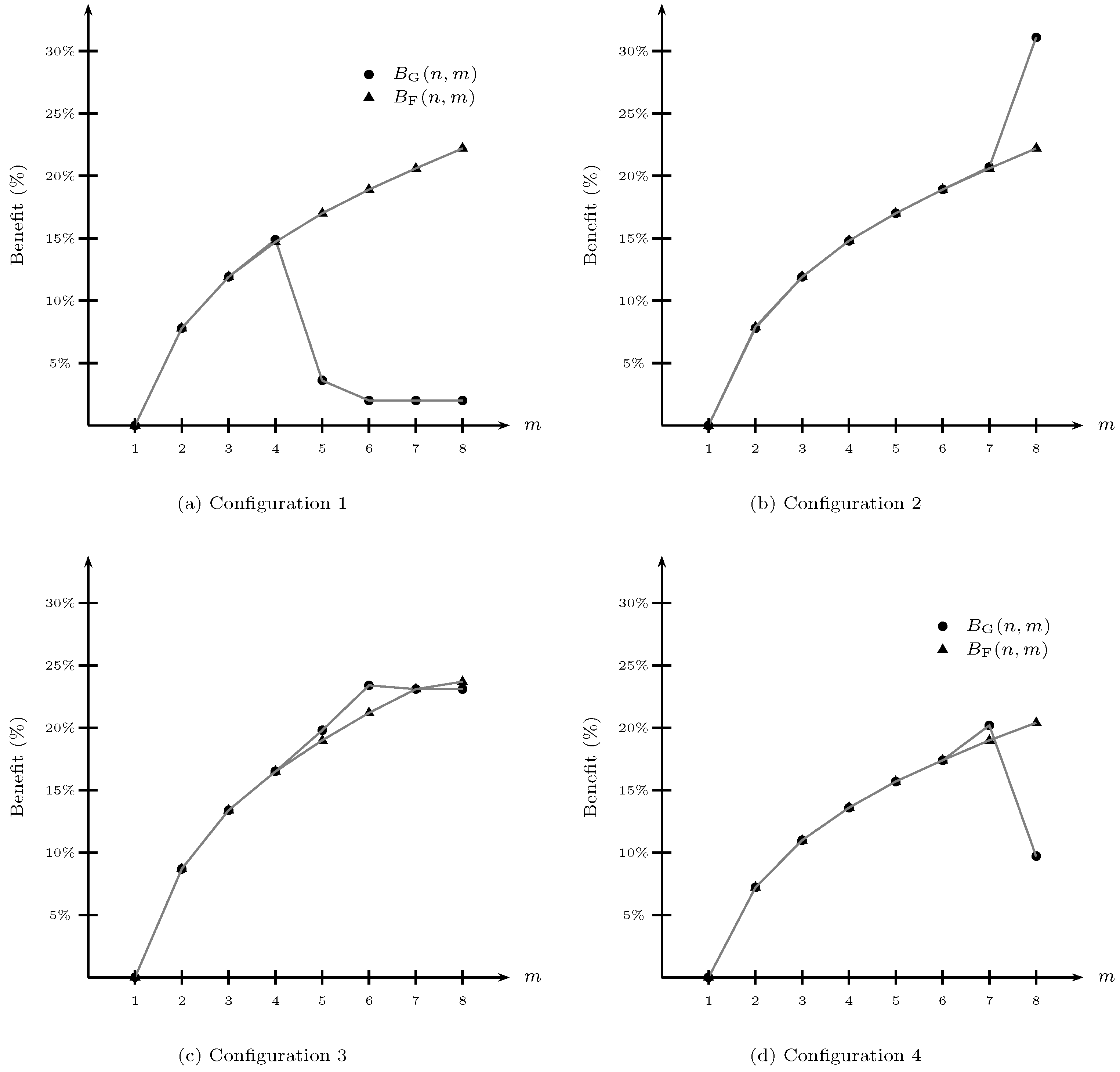
The benefit is interpreted as the percentage for which the order quantity of a single class is reduced. Note that the benefit of considering a single-class, i.e., $m=1$, will always be zero, and ${\widehat{S}}_{\mathrm{G}(n,m)}^r={\widehat{S}}_{\mathrm{F}(n,m)}^r$ for any $r=1,\dots ,M$ and $m=1$, allowing a comparison to the priority policy that yields the greater benefit. Figure 1 shows, for each demand configuration, the average benefits of grouping customer classes into different numbers of classes according to (14).

As we expected, Figure 1 shows that under GP and FLP policies, grouping all customer classes into more than a single class has a positive benefit on the order quantity (Proposition 1). The benefit is on average 22.4% and 22.1% for GP and FLP policies, respectively (Appendix F contains the details of the average and maximum benefit). In particular, under the FLP policy, the benefit monotonically increases with the number of customer classes (Proposition 2), increasing on average by 3.3% for each increase in the number of customer classes.

From Figure 1, we observe that the allocation under the GP policy is not always better than under the FLP policy. For example, when the high-priority classes dominate in terms of demand (configuration 1) and the customer classes are strictly grouped into more than four classes, the FLP policy performs better than the GP policy because $B_F(n,m)>B_G(n,m)$ for any $m=5,\dots ,8$. Under configurations 3 and 4, $B_F(n,8)>B_G(n,8)$. Unlike the case when low-priority classes dominate in terms of demand (configuration 2), the GP policy always performs better than the FLP policy, i.e., $B_F(n,m)<B_G(n,m)$ for any $m=2,\dots ,8$.

We also observe that for each configuration under the GP policy, there is an optimal number of customer classes $m^{\ast }$ such that the benefit obtained is always greater than or equal to the benefit obtained under the FLP policy. All grouping of customer classes into a number of customer classes that exceed the optimum $m^{\ast }$ will have a benefit under the FLP policy that is greater than that if the allocation is performed under the GP policy. Therefore, the optimal number of customer classes for configurations 1, 2, 3, and 4 under the GP policy are $m^{\ast }$ = 4, 8, 6, and 7 classes, respectively. In contrast, Figure 1 shows that the optimal number of customer classes under the FLP policy is to group the classes into eight customer classes for all demand configurations. This result is aligned with Proposition 2.

In particular, under the GP policy, Figure 1 shows that the maximum average benefit is achieved when the low-priority classes dominate demand (configuration 2) and the customer classes are grouped into eight classes. Its benefit has a value in excess of 30%. This occurs because the customer classes with high demand require a lower service level by increasing the number of customer classes, thus reducing the order quantity. Furthermore, under the FLP policy, Figure 1 shows that the maximum average benefit is achieved when the middle priority classes dominate demand (configuration 3) and the customer classes are grouped into eight classes. Its benefit has a value of 23.7%. Note that the benefit does not vary greatly according to the demand configuration. This is because the priority list is not built based on the demand realization;i.e., the allocation order in a shortage is defined previously.

The variation of the order quantity when grouping the customer classes into different numbers of classes is caused by the free riders and by the aggregation rule. In what follows, we quantify the effect induced by the free riders and the aggregation rule on the order quantity. We denote these effects as the free-rider effect and the cluster effect, respectively.

7.2. Free-Rider and Cluster Effects

Free-rider classes are customer classes that receive a higher service level than required. To isolate and measure the free-rider effect, we determine the variation in S by increasing the preset service level of $n-m$ customer classes to ${\overline{\alpha }}_i^{\prime }={\overline{\alpha }}_m$ for any $i=m+1,\dots ,n$. Consequently, under Sample Average Approximation, the variation of S induced by the free-rider effect is defined as:

$$F_P(n,m)={\displaystyle \frac{{\sum }_{r=1}^M\left({\displaystyle \frac{{\widehat{S}}_{P\left(n\right)}^r-{\tilde{S}}_{P(n,m)}^r}{{\widehat{S}}_{P\left(n\right)}^r}}\right)}{M}}\forall m=1,\dots ,n,$$

(15)

where ${\widehat{S}}_{\mathrm{P}\left(n\right)}^r$ is the order quantity obtained by solving the rth replication of the $\alpha {-\mathrm{SAA}}_{\mathrm{P}}\left(n\right)$ model, and ${\tilde{S}}_{\mathrm{P}(n,m)}^r$ is the order quantity obtained by solving the rth replication of the $\alpha {-\mathrm{SAA}}_{\mathrm{P}}\left(n\right)$ model with ${\overline{\alpha }}_i^{\prime }={\overline{\alpha }}_i$ for any $i=1,\dots ,m$ and ${\overline{\alpha }}_i^{\prime }={\overline{\alpha }}_m$ for any $i=m+1,\dots ,n$. The variation of the order quantity induced by the free-rider effect is the percentage at which the order quantity is only modified by providing a higher service level than that required, without modifying the number of customer classes. Under GP and FLP policies, the free-rider effect is always negative or zero, i.e., $F_P(n,m)\le 0$, because ${\widehat{S}}_{P\left(n\right)}\le {\tilde{S}}_{P(n,m)}$ for any $n>1$ and $m=1,\dots ,n$ (Proposition 3).

Table 3. Free-rider effect under GP and FLP policies, and $n=8$.

${\mathit{F}}_{\mathit{G}}(\mathit{n},\mathit{m})$
	Configuration 1		Configuration 2		Configuration 3		Configuration 4
m	Average	Max	Average	Max	Average	Max	Average	Max
1	0.0%	0.0%	−42.2%	−43.2%	−26.3%	−27.0%	−1.7%	−2.3%
2	0.0%	0.0%	−29.5%	−30.0%	−13.0%	−13.4%	0.0%	0.0%
3	0.0%	0.0%	−22.2%	−22.6%	−5.7%	−6.1%	0.0%	0.0%
4	0.0%	0.0%	−16.8%	−17.1%	−0.4%	−0.6%	0.0%	0.0%
5	0.0%	0.0%	−12.3%	−12.5%	0.0%	0.0%	0.0%	0.0%
6	0.0%	0.0%	−8.1%	−8.4%	0.0%	0.0%	0.0%	0.0%
7	0.0%	0.0%	−4.1%	−4.3%	0.0%	0.0%	0.0%	0.0%
8	0.0%	0.0%	0.0%	0.0%	0.0%	0.0%	0.0%	0.0%
${\mathit{F}}_{\mathit{F}}(\mathit{n},\mathit{m})$
	Configuration 1		Configuration 2		Configuration 3		Configuration 4
m	Average	Max	Average	Max	Average	Max	Average	Max
1	−28.5%	−29.6%	−28.6%	−29.0%	−31.1%	−32.0%	−25.6%	−26.1%
2	−18.6%	−18.9%	−18.6%	−19.0%	−19.7%	−20.2%	−16.6%	−17.0%
3	−13.2%	−13.5%	−13.2%	−13.6%	−13.6%	−13.9%	−11.8%	−12.0%
4	−9.6%	−9.8%	−9.6%	−9.9%	−9.5%	−9.7%	−8.6%	−8.8%
5	−6.7%	−6.9%	−6.7%	−7.0%	−6.2%	−6.4%	−6.0%	−6.2%
6	−4.2%	−4.4%	−4.3%	−4.4%	−3.4%	−3.5%	−3.8%	−3.9%
7	−2.0%	−2.2%	−2.1%	−2.2%	−0.9%	−0.9%	−1.8%	−1.9%
8	0.0%	0.0%	0.0%	0.0%	0.0%	0.0%	0.0%	0.0%

shows the average and maximum variation of the order quantity induced by the free-rider effect for all configurations according to (15).

As we expected, Table 3 shows that the free-rider effect is negative or zero for all configurations. We also noticed that the free-rider effect is non-increasing for the number of classes that are free-rider, i.e., ${\tilde{S}}_{P(n,m)}^r\ge {\tilde{S}}_{P(n,m+1)}^r$ for any $m=1,\dots ,7$. In particular, under the FLP policy, the free-rider effect is strictly decreasing in the number of free-rider classes, i.e., ${\tilde{S}}_{\mathrm{F}(n,m)}^r>{\tilde{S}}_{\mathrm{F}(n,m+1)}^r$ for any $m=1,\dots ,7$.

From Table 3, we observe that when high-priority classes dominate demand (configuration 1), the GP policy is absolutely robust in terms of the number of free-rider classes because the order quantity does not change even when providing the highest service level for all customer classes, i.e., $F_{\mathrm{G}}(8,m)=0$ for any $m=1,\dots ,8$. This occurs because when building the priority list under a GP policy, the customer classes with the highest demand and required service level will be located at the end of this list. Therefore, to meet their required service level, the rest of the customer classes located earlier in the priority list will receive the highest service level. In contrast, when the low-priority classes dominate demand (configuration 2), the GP policy does not accept any free-rider classes without modifying the order quantity. Table 3 also shows that the FLP policy is not robust in the number of free-rider classes because the order quantity is increasing in the number of free-rider classes. This occurs because the allocation will always follow the order of the same priority list; therefore, when attending the last customer class, which requires a greater service level as a result of being a free-rider class, the order quantity will increase.

The variation in the order quantity when grouping the customer classes into different numbers of classes is also caused by the aggregation rule that we referred to as the cluster effect. To isolate and measure the cluster effect under the low-service-level-first round-up aggregation scheme, we compute the variation induced in S by grouping $n-m$ customer classes, each of them with preset service level ${\overline{\alpha }}_i^{\prime }={\overline{\alpha }}_m$ for any $i=m+1,\dots ,n$, in a single class with preset service level ${\overline{\alpha }}_m$. Consequently, under Sample Average Approximation, the variation in S induced by the cluster effect is

$$C_{\mathrm{P}}(n,m)={\displaystyle \frac{{\sum }_{r=1}^M\left({\displaystyle \frac{{\tilde{S}}_{\mathrm{P}(n,m)}^r-{\widehat{S}}_{\mathrm{P}(n,m)}^r}{{\widehat{S}}_{\mathrm{P}\left(n\right)}^r}}\right)}{M}},\forall m=1,\dots ,n,$$

(16)

where ${\tilde{S}}_{\mathrm{P}(n,m)}^r$ is the order quantity resulting from solving the rth replication of the $\alpha {-\mathrm{SAA}}_{\mathrm{P}}\left(n\right)$ model with ${\overline{\alpha }}_i^{\prime }={\overline{\alpha }}_i$ for any $i=1,\dots ,m$ and ${\overline{\alpha }}_i^{\prime }={\overline{\alpha }}_m$ for any $i=m+1,\dots ,n$; ${\widehat{S}}_{\mathrm{P}(n,m)}^r$ is the order quantity resulting from solving the rth replication of the $\alpha {-\mathrm{SAA}}_{\mathrm{P}}(n,m)$; and ${\widehat{S}}_{\mathrm{P}\left(n\right)}^r$ is the order quantity resulting from solving the rth replication of the $\alpha {-\mathrm{SAA}}_{\mathrm{P}}\left(n\right)$ model. If this variation is positive, i.e., $C_{\mathrm{P}}(n,m)>0$ with $n>1$ and $m=1,\dots ,n$, this means that grouping customer classes in m classes reduces the order quantity.

Table 4. Cluster effect under the GP and FLP policies and $n=8$.

${\mathit{C}}_{\mathit{G}}(\mathit{n},\mathit{m})$
	Configuration 1		Configuration 2		Configuration 3		Configuration 4
m	Average	Max	Average	Max	Average	Max	Average	Max
1	−2.0%	−2.4%	−2.9%	−3.4%	−3.8%	−4.4%	−9.1%	−9.7%
2	5.9%	5.4%	−4.4%	−4.8%	−5.7%	−5.9%	−2.8%	−3.4%
3	10.1%	9.6%	−5.7%	−6.0%	−7.0%	−7.3%	1.4%	0.9%
4	13.2%	12.4%	−6.9%	−7.4%	−8.2%	−8.5%	4.3%	3.7%
5	1.7%	1.4%	−8.2%	−8.5%	−4.3%	−4.7%	6.6%	6.0%
6	0.0%	0.0%	−9.6%	−9.8%	0.4%	0.3%	8.5%	8.0%
7	0.0%	0.0%	−11.0%	−11.3%	0.0%	0.0%	11.6%	11.1%
8	0.0%	0.0%	0.0%	0.0%	0.0%	0.0%	0.0%	0.0%
${\mathit{C}}_{\mathit{F}}(\mathit{n},\mathit{m})$
	Configuration 1		Configuration 2		Configuration 3		Configuration 4
m	Average	Max	Average	Max	Average	Max	Average	Max
1	0.0%	0.0%	0.0%	0.0%	0.0%	0.0%	0.0%	0.0%
2	0.0%	0.0%	0.0%	0.0%	0.0%	0.0%	0.0%	0.0%
3	0.0%	0.0%	0.0%	0.0%	0.0%	0.0%	0.0%	0.0%
4	0.0%	0.0%	0.0%	0.0%	0.0%	0.0%	0.0%	0.0%
5	0.0%	0.0%	0.0%	0.0%	0.0%	0.0%	0.0%	0.0%
6	0.0%	0.0%	0.0%	0.0%	0.0%	0.0%	0.0%	0.0%
7	0.0%	0.0%	0.0%	0.0%	0.0%	0.0%	0.0%	0.0%
8	0.0%	0.0%	0.0%	0.0%	0.0%	0.0%	0.0%	0.0%

shows the average and maximum variation n the order quantity induced by the cluster effect for all configurations according to (16).

From Table 4, we observe that under the GP policy, there is a number of customer classes $\widehat{m}$ that have the maximum positive variation in the order quantity. Therefore, any grouping of customer classes in a number of classes other than $\widehat{m}$ yields a lower variation on the order quantity, i.e., $C_{\mathrm{G}}(8,m)<C_{\mathrm{G}}(8,\widehat{m})$ for any $m\ne \widehat{m}$. Note that the optimal number of customer classes $m^{\ast }$ that we observe in

Table A1. Benefit under the GP and FLP policies and $n=8$.

${\mathit{B}}_{\mathit{G}}(\mathit{n},\mathit{m})$
	Configuration 1		Configuration 2		Configuration 3		Configuration 4
m	Average	Max	Average	Max	Average	Max	Average	Max
1	0.0%	0.00%	0.0%	0.0%	0.0%	0.0%	0.0%	0.0%
2	7.8%	9.5%	7.8%	9.7%	8.7%	10.7%	7.2%	8.6%
3	11.9%	13.8%	11.9%	13.7%	13.4%	14.9%	11.0%	12.5%
4	14.9%	17.2%	14.8%	16.5%	16.5%	18.2%	13.6%	15.3%
5	3.6%	5.9%	17.0%	18.9%	19.8%	21.5%	15.7%	17.4%
6	2.0%	4.2%	18.9%	20.6%	23.4%	25.4%	17.4%	19.3%
7	2.0%	4.2%	20.7%	22.3%	23.1%	25.1%	20.2%	22.6%
8	2.0%	4.2%	31.1%	33.2%	23.1%	25.1%	9.7%	12.3%
${\mathit{B}}_{\mathit{F}}(\mathit{n},\mathit{m})$
	Configuration 1		Configuration 2		Configuration 3		Configuration 4
m	Average	Max	Average	Max	Average	Max	Average	Max
1	0.0%	0.0%	0.0%	0.0%	0.0%	0.0%	0.0%	0.0%
2	7.8%	9.5%	7.9%	9.7%	8.7%	10.7%	7.2%	8.6%
3	11.9%	13.8%	11.9%	13.7%	13.4%	14.9%	11.0%	12.5%
4	14.7%	16.6%	14.8%	16.5%	16.5%	18.2%	13.6%	15.3%
5	17.0%	18.8%	17.0%	18.9%	19.0%	20.7%	15.7%	17.4%
6	18.9%	20.5%	18.9%	20.6%	21.2%	22.9%	17.4%	19.3%
7	20.6%	22.2%	20.6%	22.3%	23.1%	24.8%	19.0%	20.8%
8	22.2%	23.6%	22.2%	23.8%	23.7%	25.4%	20.4%	22.3%

matches the number of classes that have maximum positive variation, i.e., $m^{\ast }=\widehat{m}$. In contrast, under the FLP policy, Table 4 shows that there is no variation in the order quantity for the grouping of customer classes into fewer classes providing the same service level. This occurs because the priority list built under an FLP policy is the same for both problems. Therefore, the order quantity will not change if there are no modifications in the service level required by any customer class.

The total variation in the order quantity produced by grouping customer classes according to the low-service-level-first-rule round-up aggregation scheme in m classes, instead of grouping them in n classes, is the sum of the free-rider (15) and cluster effects (16), i.e.,

$$F_{\mathrm{P}}(n,m)+C_{\mathrm{P}}(n,m)={\displaystyle \frac{{\sum }_{r=1}^M\left({\displaystyle \frac{{\widehat{S}}_{\mathrm{P}\left(n\right)}^r-{\widehat{S}}_{\mathrm{P}(n,m)}^r}{{\widehat{S}}_{\mathrm{P}\left(n\right)}^r}}\right)}{M}}.$$

From Table 3 and Table 4, we observe that when high-priority classes dominate demand (configuration 1), the total variation in the order quantity S under the GP policy is totally caused by the cluster effect, while for configurations 2, 3, and 4, the total variation of the order quantity S is caused by both effects. Note that the total variation in the order quantity under the GP policy by grouping customer classes in $\widehat{m}$ instead of n classes is only caused by the cluster effect, given that under the same number of customer classes $\widehat{m}$, the free-rider effect is null under the GP policy. In contrast, from Table 3 and Table 4, we observe that the total variation in the order quantity S under the FLP policy, for all configurations, is only caused by the free-rider effect because the cluster effect is null under the FLP policy.

7.3. Performance of Sample Average Approximation

To measure the quality solutions resulting from solving the SAA problems, the optimality gap is determined according to (13) using the minimum value of the M replicates as a lower bound and verifying the feasibility of the highest value of these replicates. In the case of non-feasibility, this value is increased by $0.1\%$ until it meets the established condition and is considered a feasible solution and the upper bound. The values are, at least with $99.9\%$ probability, the lower and upper bounds of the problem. 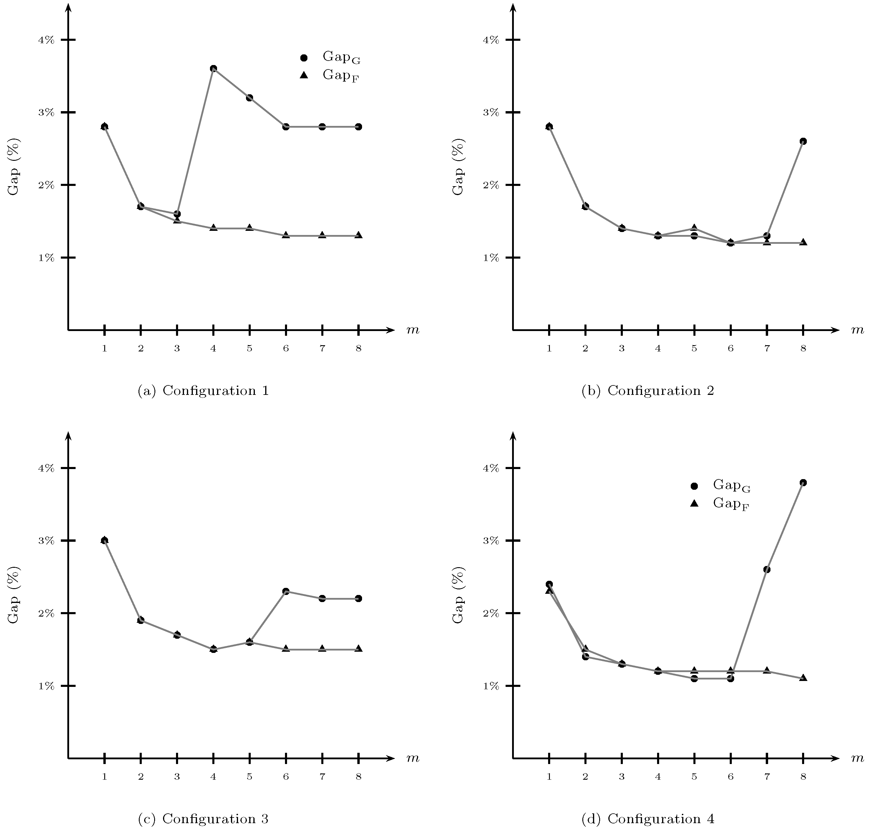Figure 2 shows, for each demand configuration, the average relative optimality gap of the feasible solution, ${\widehat{S}}_{\mathrm{P}\left(n\right)}$, resulting from the SAA method and using the $\alpha {-\mathrm{SAA}}_{\mathrm{P}}(n,m)$ model with $m=1,\dots ,8$, under the GP and FLP policies.

From Figure 2, we observe that the average optimality gap of the feasible solution ${\widehat{S}}_{\mathrm{P}\left(n\right)}$ is decreasing with m under a GP policy. Furthermore, the magnitude of the average optimality gap under the GP policy does not vary with the demand configurations. On the other hand, the average optimality gap under the FLP policy decreasesand then increases with m. The inflection coincides, for each demand configuration, with the inflection of the benefit of grouping customer classes into different numbers of classes (Figure 1).

We observe that the SAA method has a good performance in terms of solving the greedy and fixed-list service level problems because the maximum optimality gap is $4.8\%$ and $4.5\%$ under GP and FLP policies, respectively.

Table A2. Optimality gap under the GP and FLP policies with $n=8$.

${\mathit{Gap}}_{\mathit{G}}$(%)
	Configuration 1		Configuration 2		Configuration 3		Configuration 4
m	Average	Max	Average	Max	Average	Max	Average	Max
1	2.8%	3.5%	2.8%	3.7%	3.0%	4.8%	2.4%	3.1%
2	1.7%	2.3%	1.7%	2.4%	1.9%	2.5%	1.4%	2.2%
3	1.6%	2.1%	1.4%	2.1%	1.7%	2.2%	1.3%	1.7%
4	3.6%	4.8%	1.3%	1.8%	1.5%	2.4%	1.2%	1.6%
5	3.2%	4.5%	1.3%	1.7%	1.6%	2.3%	1.1%	1.4%
6	2.8%	4.7%	1.2%	1.6%	2.3%	3.1%	1.1%	1.4%
7	2.8%	4.7%	1.3%	1.5%	2.2%	3.1%	2.6%	4.6%
8	2.8%	4.7%	2.6%	3.6%	2.2%	3.1%	3.8%	4.6%
${\mathit{Gap}}_{\mathit{F}}$(%)
	Configuration 1		Configuration 2		Configuration 3		Configuration 4
m	Average	Max	Average	Max	Average	Max	Average	Max
1	2.8%	3.9%	2.8%	3.5%	3.0%	4.5%	2.3%	3.2%
2	1.7%	2.6%	1.7%	2.4%	1.9%	2.3%	1.5%	2.2%
3	1.5%	2.3%	1.4%	2.1%	1.7%	2.1%	1.3%	1.9%
4	1.4%	2.0%	1.3%	1.8%	1.5%	2.0%	1.2%	1.7%
5	1.4%	1.9%	1.4%	1.7%	1.6%	2.0%	1.2%	1.7%
6	1.3%	1.8%	1.2%	1.8%	1.5%	2.2%	1.2%	1.6%
7	1.3%	1.8%	1.2%	1.6%	1.5%	1.9%	1.2%	1.7%
8	1.3%	1.9%	1.2%	1.7%	1.5%	2.0%	1.1%	1.6%

in Appendix G contains the average and maximum optimality gap for each demand configuration and priority policy.

8. Conclusions

This paper studies the effect that the number of customer classes has on the order quantity under a single-period inventory system with stochastic demand and individual $\alpha$ service-level requirements from multiple customer classes. We formulated multi-customer class service-level problems under greedy and fixed-list priority policies as nonlinear problems with chance constraints. These problems are difficult to solve for more than three customer classes. Consequently, we have proposed a reformulation of models as MIP using a Sample Average Approximation approach, which allowed us to obtain results for up to eight customer classes in reasonable computational times. The computational results show that the Sample Average Approximation method is able to identify good-quality solutions because, for the tested instances, the maximum optimality gap was 4.8%, which is a very good solution.

To determine the effect of the number of customer classes on the inventory level under greedy and fixed-list priority policies, we considered a round-up aggregation scheme that does not harm the service level of the aggregated classes. Under such a policy, the variation in the order quantity when grouping the customers into different numbers of customer classes is caused by the free-rider classes (free-rider effect) and by the aggregation rule (cluster effect).

Under a low-service-level-first-rule round-up aggregation scheme, several properties of the models were proven, from which we obtained the following managerial insights.

• Under greedy and fixed-list priority policies, grouping all customer classes in a single class with the highest preset service level induces the largest optimal order quantity. Therefore, grouping customers into more than one class has a positive effect on the order quantity.
• The order quantity induced by the fixed-list priority policy is non-increasing with the number of customer classes.
• The order quantity induced by the greedy and fixed-list priority policies is non-decreasing with the number of free-rider classes.

We conducted several test problems under low-service-level-first-rule round-up aggregation scheme and different demand configurations of customer classes, from which we observed the following managerial insights.

• When the high-priority classes dominate demand and customers are grouped into strictly more than four classes, the fixed-list priority policy performs better than the greedy priority policy; i.e., allocating resources under greedy priority policy is not always better than that of the fixed-list priority policy.
• When the low-priority classes dominate demand, the greedy priority policy always performs better than the fixed-list priority policy.
• Under greedy and fixed-list priority policies, the optimal number of customer classes is greater than or equal to four classes. Therefore, for the instances we tested, it was not optimal to group the customers into two or three customer classes using, for example, Pareto or ABC classification.
• When high-priority classes dominate demand, the total variation of the order quantity, when grouping customers into different numbers of customer classes under greedy priority policy is totally caused by the cluster effect. For other demand configurations, the total variation in the order quantity is caused by cluster and free-rider effects.
• Under greedy priority policy, the total variation of the order quantity when grouping customers into the optimal number of customer classes is totally caused by the cluster effect because, under the same number of customer classes, the free-rider effect is null.
• Under the fixed-list priority policy, the total variation of the order quantity when grouping customers into different numbers of customer classes is totally caused by the free-rider effect because the cluster effect is null under fixed-list policy.
• When the high-priority classes dominate demand, greedy priority policy is absolutely robust in the number of free-rider classes because there is no variation in the order quantity by increasing the number of free-rider classes.

In this way, we have answered the research questions posed at the beginning of this document. A brief response for each research question is the following. (i) How does the number of customer classes affect the inventory level under different priority policies? From Figure 1, we can see that under the greedy priority policy, the inventory level depends on the demand configuration, having in all configurations a number of classes that minimizes the inventory level. Here there is no monoticity. Under a fixed-list priority policy, the inventory level is non-increasing in the number of classes for all the configurations. (ii) What is the optimal number of customer classes under different demand configurations? According to Figure 1, for the greedy priority policy, the optimal number depends on the configuration of the demand, but we can observe that when the demand is dominated by the high-priority classes (configuration 1), the optimal number of classes is smaller than when the demand is dominated by the low-priority classes (configuration 2). For the fixed-list priority approach, the optimal number is always the maximum number of classes that can be had. (iii) What priority policy performs better under different demand configurations? When the high-priority classes dominate in terms of demand (configuration 1) and the customer classes are strictly grouped into more than four classes, the fixed-list priority policy performs better than the greedy priority policy. When the low-priority classes dominate in terms of demand (configuration 2), the greedy priority policy always performs better than the fixed-list priority policy.

There are two main questions left for future research. The first one is to determine the best aggregation rule under a round-up scheme because the low-service-level-first-rule is not the only aggregation rule under a round-up scheme. Other aggregation rules include the high-service-level-first-rule and the random-rule. The second issue is to determine how different priority policies, such as the largest-debt-first policy of Zhong et al. [9] or the max-weighted-service policy of Jiang et al. [12], affect the number of customer classes in a single-period inventory system. A final issue is to address the risk of using responsive priority policies because, under these types of policies, the priority list in case a shortage is not previously known by customers or offers.

Finally, this contribution is intended to be useful for managers seeking guidelines for grouping their customers, as well as for academics seeking to investigate the performance of different configurations of customer service policies.