A Martingale Posterior-Based Fault Detection and Estimation Method for Electrical Systems of Industry

Abstract

The improvement of information sciences promotes the utilization of data for process monitoring. As the core of modern automation, time-stamped signals are used to estimate the system state and construct the data-driven model. Many recent studies claimed that the effectiveness of data-driven methods relies greatly on data quality. Considering the complexity of the operating environment, process data will inevitably be affected. This poses big challenges to estimating faults from data and delivers feasible strategies for electrical systems of industry. This paper addresses the missing data problem commonly in traction systems by designing a martingale posterior-based data generation method for the state-space model. Then, a data-driven approach is proposed for fault detection and estimation via the subspace identification technique. It is a general scheme using the Bayesian framework, in which the Dirichlet process plays a crucial role. The data-driven method is applied to a pilot-scale traction motor platform. Experimental results show that the method has good estimation performance.

1. Introduction

With the increasing demand for production efficiency, the construction and optimization of industrial processes have received great attention [1,2,3]. In the actual industry, ensuring the safety of systems and equipment is an important quality indicator of service. As the vital factor in industrial process, electrical systems have the advantages of multiple functions, high integration and high intelligence [4,5,6]. With the accumulation of service time, the safety and reliability of mechatronics gradually decreases due to the degradation of system performance. Consequently, developing effective fault detection (FD) and fault estimation (FE) methods is of great significance for improving the stability of systems [7].

Traditional model-based methods for FD and FE usually require some prior knowledge to obtain accurate results. However, it is tough to obtain accurate physical models for complex industrial systems. Data-driven methods do not require the establishment of system models nor the estimation of parameters through first principles, which has a natural advantage in the era of big data [8]. It has better applicability to electrical systems with high complexity and strong coupling characteristics. From the currently published results, it can be found that data-driven methods can be divided into two categories: the multivariate statistic analysis-based method (MSAM) and the subspace identification-based method (SIM) [9]. Many popular MSAMs such as principal component analysis (PCA) [10], partial least squares (PLS) [11], and canonical correlation analysis (CCA) [12] realize process monitoring and fault diagnosis through statistical analysis. they have the advantage of simplicity and efficiency when addressing big data. Oriented towards the needs of large-scale monitoring, many improved MSAMs have been introduced in recent years, such as the sparse integrated dynamic PCA [13], adaptive mean PCA [14], local tangent space alignment PCA and CCA [15,16], and slow feature analysis [17].

Subspace identification-based data-driven methods, one of the commonly used techniques recently, reduce the need for causality by parameter identification from stacked input and output signals easily. The base of this type of method is a state-space model, which implements iterative estimation with a Kalman filter. It can discover the interactive effects through the propagation of faults. In [18], the data-driven stable kernel representation (SKR) and stable image representation (SIR) are introduced for dynamic systems. It is a fundamental study for FD using the data-driven observer framework. For sensor faults in automatized industrial systems, a subspace-aided fault diagnosis and compensation control approach via SKR and SIR  is used [19]. In [20], two sparse models are formulated and data models are introduced for cyber-physical systems under sparse actuator attacks. Based on this approach, a subspace-aided FD for identifying the data-driven SKR of a closed-loop system is constructed. Considering the noise problem in rolling mill processes with eccentricity, a robust subspace-aided FD is proposed. By utilizing the prior information and generalized orthonormal basis functions, a continuous-time subspace identification method is proposed in [21]. In addition, there are lots of studies designing data-driven methods considering determining disturbances. In [22], a just-in-time learning-based data-driven FD framework for nonlinear processes with deterministic disturbances is proposed. In [23], an alternative FD scheme is proposed. This method of residual generation avoids the identification process and provides an effective solution to address deterministic disturbances. In [24], by projecting the process data into the determined subspaces, the FD systems can be designed via the identified kernel subspace of systems.

For fault estimation (FE) problems of dynamic systems, a state-space model can also be used as an effective tool. It provides a basis for designing of fault compensation [25]. At present, most FE schemes construct observer-based methods and utilize well-established identification techniques. In [26], optimal observer-based FE for Takagi–Sugeno fuzzy systems with process faults is proposed. Aiming at improving the sensitivity and robustness to faults, a least squares FE scheme is developed. In [27], a distributed FE observer is designed for subsystems after the decoupling of external disturbances. In addition, many studies regard FE as the first step of fault-tolerant control and adjust the controller by estimating the value to achieve stable control [28,29,30]. In addition, some other studies on fault identification are similar to those on FE. All of them estimate the fault amplitude by fault characteristics. In [31], a collaborative deep learning framework is proposed for dynamic systems. It can accomplish the effective estimation for system faults. In [32], a novel fault section identification framework developed by entropy is designed for avoiding the false operation of converter station protection. The adaptation is studied by considering the position, type, and angle of faults. Studies in [33,34,35,36,37] accomplished fault identification for improving the running performance of a traction motor with different types of models. In [38], to reduce the limitations of the fault identification of an arc, a novel method for evaluating the transient and steady dynamic states of arcing faults via a time–frequency analysis was constructed. It is worth noting that the definition of fault identification is different in studies, and quite a number of studies define it as fault isolation, which is different from the content of this paper [39,40,41,42]. Although these methods can obtain accurate results, the missing data problem that cannot be ignored in the industrial process greatly affects the accuracy of data-driven methods [43,44,45]. The classical solution to this issue is to analyze the missing mechanism and deal with it using imputation algorithms. This interpolation solution cannot reduce the uncertainty of the model in data-driven frameworks. Designing a data imputation scheme from the perspective of a sampling distribution can obtain more stable results in the framework of Kalman filtering. Considering the problems summarized above, the contributions of this paper can be concluded as follows.

(1)

A martingale posterior-based (MP) data generation method is introduced for electrical systems of industry. The Dirichlet process is considered to analyze the complex distribution problem in the generation process.

(2)

The data-driven scheme is designed via MP and SKR. It not only ensures the recursive realization of estimation but improves the modeling accuracy by reducing the uncertainty.

(3)

FD and FE, using the proposed framework for electrical systems of industry, are accomplished, respectively.

The rest of this paper is given below. The basic methods and current problems are summarized in the Preliminaries section, shown in the Section 2. The proposed FD and FE methods, using MP, are introduced in Section 3. Experiments and discussions for verification and comparison are outlined in Section 4. The conclusions and future directions of this work are shown in Section 5.

Notations: $S_{LTI}$ signifies a linear time-invariant dynamic system; $S_f$ represents the dynamic systems with faults and missing data; x represents the state of systems; ${\mathbb{R}}^a$ represents the a-dimensional Euclidean space; $\widehat{x}$ represents the estimation of x.

2. Preliminaries and Problem Formulation

In this section, the observer-based data-driven FD is introduced and the objects of this study is summarized.

2.1. Observer-Based Data-Driven FD

Considering the linear time-invariant dynamic system, its state-space model can be given by

$$S_{LTI}:\left\{\begin{array}{c}x(k+1)=Ax\left(k\right)+Bu\left(k\right)+w\left(k\right)\hfill \\ y\left(k\right)=Cx\left(k\right)+v\left(k\right)\hfill \end{array}\right.$$

(1)

where k represents the sampling instant; $x\in {\mathbb{R}}^{k_x}$ is the state of dynamic systems; $u\in {\mathbb{R}}^{k_u}$ and $y\in {\mathbb{R}}^{k_y}$ are the input and output of dynamic systems, respectively; and A, B, and C are known matrices with appropriate dimensions. They can be understood as transfer matrices in Markov processes. $w\in {\mathbb{R}}^{k_x}$ and $v\in {\mathbb{R}}^{k_y}$ represent the process noise and measurement noise, respectively. They are independent of x.

Based on the model (1), the system with faults and missing data becomes

$$S_f:\left\{\begin{array}{c}x(k+1)=Ax\left(k\right)+Bu\left(k\right)+w\left(k\right)+F_1{f}_1\left(k\right)\hfill \\ y\left(k\right)=Cx\left(k\right)+v\left(k\right)+F_2{f}_2\left(k\right),y\in {\Omega }_y\hfill \end{array}\right.$$

(2)

where $f_1$ and $f_2$ are, respectively, the process and sensor faults; $F_1$ and $F_2$ represent the parameter matrices of appropriate dimensions. ${\Omega }_y$ is the real number set, representing the collected output samples.

To detect faults in (2), a state observer and residual generator r are introduced as follows.

$${\widehat{S}}_{LTI}:\left\{\begin{array}{c}\widehat{x}(k+1)=A\widehat{x}\left(k\right)+Bu\left(k\right)\hfill \\ \widehat{y}\left(k\right)=C\widehat{x}\left(k\right)+v\left(k\right)\hfill \end{array}\right.$$

(3)

$$y\left(k\right)-\widehat{y}\left(k\right)=r\left(k\right)\left\{\begin{array}{c}=0,forS\hfill \\ \ne 0,for{S}_f\hfill \end{array}\right.$$

(4)

Due to the system state $x\left(k\right)$ in (1) being a latent variable that cannot be directly measured by sensors in reality, the data-driven scheme enables the parameter identification of a residual generator with the input and output data of systems. The following introduces an important operator SKR, which realizes the mapping of input and output signals to residual signals.

$$\mathcal{K}:\left\{\begin{array}{c}r\left(k\right)=\mathcal{K}\left(\begin{array}{c}u\left(k\right)\hfill \\ y\left(k\right)\hfill \end{array}\right)=0,forS\hfill \\ r_f\left(k\right)={\mathcal{K}}_f\left(\begin{array}{c}u\left(k\right)\hfill \\ y\left(k\right)\hfill \end{array}\right)\ne 0,for{S}_f\hfill \end{array}\right.$$

(5)

2.2. Bayesian Filter for State Estimation

As the basis of the Kalman filtering method, the Bayesian filtering method has been widely studied in medical treatment [46], navigation [47], radar systems [48], and electrical systems [49]. The basic framework is given as follows.

In a Bayesian filter framework, the belief of the prior of a state can be expresses as

$$Be{l}_{prior}\left(x\left(k\right)\right)=p(\left.x\left(k\right)\right|y\left(1\right),y\left(2\right),\cdots y(k-1),u\left(1\right),u\left(2\right),\cdots u\left(k\right))$$

(6)

Then, the belief of the posterior of a state is

$$Be{l}_{posterior}\left(x\left(k\right)\right)=p(\left.x\left(k\right)\right|y\left(1\right),y\left(2\right),\cdots y\left(k\right),u\left(1\right),u\left(2\right),\cdots u\left(k\right))$$

(7)

The result obtained by the total probability formula is

$$\begin{array}{c}Be{l}_{prior}\left(x\left(k\right)\right)=\sum p(\left.x\left(k\right)\right|x(k-1),y\left(1\right),\cdots y(k-1),u\left(1\right),\cdots u\left(k\right))\hfill \\ \ast p(\left.x(k-1)\right|x(k-1),y\left(1\right),\cdots y(k-1),u\left(1\right),\cdots u\left(k\right))\hfill \end{array}$$

(8)

Therefore, the following equation is true.

$$\begin{array}{c}Be{l}_{prior}\left(x\left(k\right)\right)=p(\left.x\left(k\right)\right|y\left(1\right),\cdots y(k-1),u\left(1\right),\cdots u\left(k\right))\hfill \\ =\sum p(\left.x\left(k\right)\right|x(k-1),u\left(k\right))\ast p(\left.x(k-1)\right|y\left(1\right),\cdots y(k-1),u\left(1\right),\cdots u\left(k\right))\hfill \end{array}$$

(9)

In the end, the prior of probability is

$$Be{l}_{prior}\left(x\left(k\right)\right)=\sum p(\left.x\left(k\right)\right|x(k-1),u\left(k\right))\ast Be{l}_{prior}\left(x(k-1)\right)$$

(10)

Under the condition of the Markov model, the state transition probability of the system can be expressed as

$$p(\left.x\left(k\right)\right|x(k-1),u\left(k\right))=p(\left.x\left(k\right)\right|x\left(0\right),\cdots x(k-1),y\left(1\right),y\left(2\right),\cdots y(k-1),u\left(1\right),u\left(2\right),\cdots u\left(k\right))$$

(11)

From the relations between state and measurement, it has

$$p\left(\left.y\left(k\right)\right|x\left(k\right)\right)=p(\left.y\left(k\right)\right|x\left(0\right),\cdots x\left(k\right),y\left(1\right),y\left(2\right),\cdots y(k-1),u\left(1\right),u\left(2\right),\cdots u\left(k\right))$$

(12)

According to the Bayesian rules, the posterior of state $x\left(k\right)$ is

$$\begin{array}{c}p(\left.x\left(k\right)\right|y\left(1\right),y\left(2\right),\cdots y\left(k\right),u\left(1\right),u\left(2\right),\cdots u\left(k\right))\hfill \\ ={\displaystyle \frac{p(\left.y\left(k\right)\right|x\left(k\right),y\left(1\right),\cdots y(k-1),u\left(1\right),\cdots u\left(k\right))\ast p(\left.x\left(k\right)\right|y\left(1\right),\cdots y(k-1),u\left(1\right),\cdots u\left(k\right))}{p(\left.y\left(k\right)\right|y\left(1\right),\cdots y(k-1),u\left(1\right),\cdots u\left(k\right))}}\hfill \end{array}$$

(13)

By the nature of Markov chains, it has

$$\begin{array}{c}p(\left.x\left(k\right)\right|y\left(1\right),y\left(2\right),\cdots y\left(k\right),u\left(1\right),u\left(2\right),\cdots u\left(k\right))\hfill \\ =p(\left.y\left(k\right)\right|y\left(1\right),y\left(2\right),\cdots y(k-1),u\left(1\right),u\left(2\right),\cdots u\left(k\right))\hfill \\ \ast p\left(\left.y\left(k\right)\right|x\left(k\right)\right)\ast p(\left.x\left(k\right)\right|y\left(1\right),\cdots y(k-1),u\left(1\right),\cdots u\left(k\right))\hfill \end{array}$$

(14)

2.3. Problem Formulation

Currently, the problem of missing data in a system is usually solved by calculating interpolation through a mechanism analysis. Due to the complexity and coupling of the system, it is excessively costly to obtain a reliable mechanism. Therefore, how to quantify the uncertainty of the data-driven model to improve the accuracy of data augmentation is an important research issue. From the designing process of the data-driven observer, it can be found that the Kalman filter framework with the Bayesian method as the core has a good noise reduction estimation ability. However, calculating posterior estimation will inevitably lead to discussing prior uncertainty. As an extension of the prediction distribution problem, this study regards the uncertainty problem as the missing problem of $y_{n+1:\infty }$. It tries to improve the data-driven FD and FE scheme through the augmentation method.

Motivated by the analysis above, the main problems of this study should be solved as follows.

• To design a data generation method for reducing uncertainty in dynamic system models.
• To construct a data-driven model that is suitable for dynamic systems with a missing data problem.
• To finish the FD and FE tasks for electrical systems of industry.

3. The MP-Based FD and FE Methods

In this section, the MP-based FE and FE methods are proposed for systems (2) with the Dirichlet process and subspace identification technique. The specific flow chart is shown in Figure 1.

3.1. MP-Based Data Generation

As an alternative of Bayesian inference, the MP can be used to quantify the uncertainty of a model [50]. This method assumes that future observations $y_{n+1:\infty }$ are generated by a hypothetical distribution ${\mathbb{P}}_{\infty }$. The MP is defined as

$${\theta }_n\left(\xi \right)=\int {\xi }^{*}\left(y_{1:\infty }\right)d{\mathbb{P}}_{\infty }\left(y_{n+1:\infty }\left|y_{1:n}\right.\right)$$

(15)

where ${\xi }^{*}\left(y_{1:\infty }\right)$ is the estimator of $\xi$ if $y_{1:\infty }$ is given. In the traditional Bayesian framework, Dirichlet processes are often used for prior probability calculations. In this study, they are utilized to obtain the posterior probability of the completed samples. Some critical properties of the Dirichlet process are summarized in [51]. ${\theta }_n\left(\xi \right)$ converges to the Dirac measure centered at the $\xi$ as $n\to \infty$. Therefore, the posterior probability sample can be constructed through the following Dirichlet process.

$$F_{\infty }\sim DP(c+n,{\displaystyle \frac{cD+{\displaystyle \sum _{i=1}^n}{\delta }_{y_i}}{c+n}})$$

(16)

where D represents the base measure. c is the concentration parameter. It has $F_{\infty }:={\displaystyle \sum _{i=1}^n}{\omega }_i{\delta }_{y_i}+{\displaystyle \sum _{i=n+1}^{\infty }}{\omega }_i{\delta }_{{\rho }_i}$, with ${\rho }_i\sim D$. The generated samples can be seen as a weighted combination of repeated empirical observations and samples from a specified distribution. They can be understood as a combination problem of samples in different distributions. The distribution assumption under the Bayesian framework can be avoided via this solution.

The missing samples can be obtained from the MP as follows.

$$\begin{array}{c}{y}_m=arg\underset{\xi }{min}\int l_{\xi }\left(y_{1:\infty }\right)d{F}_{\infty }\left(y_{1:\infty }\right)\hfill \\ =arg\underset{\xi }{min}{\displaystyle \sum _{i=1}^n}{\omega }_i{\delta }_{y_i}+{\displaystyle \sum _{i=n+1}^{\infty }}{\omega }_i{\delta }_{{\rho }_i}\hfill \end{array}$$

(17)

3.2. Identification of Data-Driven Model

To accomplish the data-driven designs of FD and FE, an I/O model based on data generation is introduced. Let $\gamma \left(k\right)\in {\mathbb{R}}^{\gamma }$ be a vector; the specific data stacking model is given below.

$$\begin{array}{c}{\gamma }_s\left(k\right)=\left[\begin{array}{c}\gamma \left(k\right)\hfill \\ ⋮\hfill \\ \gamma (k+s)\hfill \end{array}\right]\in {\mathbb{R}}^{(s+1)\gamma },{\mathrm{\Gamma }}_k=\left[\begin{array}{ccc}\gamma \left(k\right)& \cdots & \gamma (k+N-1)\end{array}\right]\in {\mathbb{R}}^{\gamma \times N}\hfill \end{array}$$

(18)

$$\begin{array}{c}{\mathrm{\Gamma }}_{k,s}=\left[\begin{array}{ccc}{\gamma }_s\left(k\right)& \cdots & {\gamma }_s(k+N-1)\end{array}\right]=\left[\begin{array}{c}{\mathrm{\Gamma }}_k\hfill \\ ⋮\hfill \\ {\mathrm{\Gamma }}_{k+s}\hfill \end{array}\right]\in {\mathbb{R}}^{(s+1)\gamma \times N}\hfill \end{array}$$

(19)

where s and N are large integers. Based on these data-stacking methods, the improved I/O data model can be described by

$$Y_{k,s}^c={\mathrm{\Lambda }}_s{X}_s+H_{u,s}{U}_{k,s}+H_{w,s}{W}_{k,s}+V_{k,s}\in {\mathbb{R}}^{(s+1)m\times N}$$

(20)

where

$$\begin{array}{c}{\mathrm{\Lambda }}_s=\left[\begin{array}{c}C\hfill \\ CA\hfill \\ ⋮\hfill \\ C{A}^s\hfill \end{array}\right]\in R^{(s+1)m\times n},H_{u,s}=\left[\begin{array}{c}\begin{array}{cccc}D& 0& & \end{array}\hfill \\ \begin{array}{cccc}CB& \ddots & \ddots & \end{array}\hfill \\ \begin{array}{cccc}⋮& \ddots & \ddots & 0\end{array}\hfill \\ \begin{array}{cccc}C{A}^{s-1}B& \cdots & CB& D\end{array}\hfill \end{array}\right].\hfill \end{array}$$

(21)

It should be noted that $Y_{k,s}^c$ in (11) can be divided into two parts: one is the measurement value directly collected by the sensor and the other is the missing value calculated by (8). Due to the relationship between $Y_{k,s}^c$ and ${\widehat{Y}}_{k,s}^c$, the I/O model with missing data can be described in

$$Y_{k,s}^c={\Phi }_{s,\eta -1}^K{Z}_{k-\eta ,\eta -1}+H_{y,s}^K{Y}_{k,s}^c+H_{u,s}^K{U}_{k,s}+E_{k,s}$$

(22)

where

$$\begin{array}{c}{\Phi }_{s,\eta -1}^K=\left[\begin{array}{cc}{\Phi }_{s,\eta -1,u}^K& {\Phi }_{s,\eta -1,y}^K\end{array}\right]\hfill \\ {\Phi }_{s,\eta -1,u}^K={\mathrm{\Lambda }}_s^K\left[\begin{array}{ccc}{A}_K^{\eta -1}{B}_K& \cdots & B_K\end{array}\right]\hfill \\ {\Phi }_{s,\eta -1,y}^K={\mathrm{\Lambda }}_s^K\left[\begin{array}{ccc}{A}_K^{\eta -1}K& \cdots & K\end{array}\right]\hfill \end{array}$$

(23)

In (23), $A_K=A-KC$ and $B_K=B-KD$. The parameter K represents the Kalman gain. $\eta$ is a large integer. In addition, $Y_k^c$ can be represented as

$$\begin{array}{c}{Y}_k^c\approx {\displaystyle \sum _{i=1}^{s+\eta }}C{A}_K^{i-1}\left[\begin{array}{cc}{B}_K& K\end{array}\right]\left[\begin{array}{c}{U}_{k-i}\hfill \\ Y_{k-i}\hfill \end{array}\right]+D{U}_k+E_k\hfill \\ E_k=\left[\begin{array}{ccc}e\left(k\right)& & e(k+N-1)\end{array}\right]\hfill \end{array}$$

(24)

To identify the parameters of the data model, singular value decomposition (SVD) is introduced to finish the least square estimation using process data. The parameter identification of the data model can be described as follows.

$$\left[\begin{array}{c}{Z}_{k-s_p,s_p-1}\hfill \\ U_{k,s}\hfill \\ Y_{k,s}^c\hfill \end{array}\right]={\left[\begin{array}{c}{S}_1\hfill \\ S_2\hfill \\ S_3\hfill \\ S_4\hfill \end{array}\right]}^T\times \left[\begin{array}{c}\begin{array}{cccc}\sum _{U_0}& & & \end{array}\hfill \\ \begin{array}{cccc} & \sum _{Y_0^c}& & \end{array}\hfill \\ \begin{array}{cccc} & & \sum _{U_1}& \end{array}\hfill \\ \begin{array}{cccc} & & & \sum _{Y_1^c}\end{array}\hfill \end{array}\right]\times \left[\begin{array}{c}{V}_1^T\hfill \\ V_2^T\hfill \\ V_3^T\hfill \\ V_4^T\hfill \end{array}\right]$$

(25)

Therefore, the parameter can be determined by

$$\left[\begin{array}{cc}{\Phi }_{s,\eta -1}& H_{u,s}\end{array}\right]=S_4\sum V^T{\left[\begin{array}{c}{S}_3\sum V^T\hfill \\ \left[\begin{array}{c}{S}_1\hfill \\ S_2\hfill \end{array}\right]\sum V^T\hfill \end{array}\right]}^{†}$$

(26)

3.3. FD and FD for Electrical Systems

By using the parameters identified in (17), a residual generator for FD and FE can be given as

$$\begin{array}{c}{R}_{k,s}=Y_{k,s}^c-{\widehat{Y}}_{k,s}^c\hfill \\ =Y_{k,s}^c-S_4\sum V^T{\left[\begin{array}{c}{S}_3\sum V^T\hfill \\ \left[\begin{array}{c}{S}_1\hfill \\ S_2\hfill \end{array}\right]\sum V^T\hfill \end{array}\right]}^{†}\left[\begin{array}{c}{Z}_{k-\eta ,\eta -1}\hfill \\ U_{k,s}\hfill \end{array}\right]\hfill \end{array}$$

(27)

FD of systems can be realized through the residual signal R. The residual signal $R_t$ calculated by fault-free systems can be used as the threshold for FD, which can be expressed as

$$\begin{array}{c}{H}_0:R_t-R\le 0\Rightarrow fault-free\hfill \\ H_1:R_t-R>0\Rightarrow faulty\hfill \end{array}$$

(28)

In addition, considering that the data-driven methods analyze the dynamic performance of systems via data stacking, the accuracy of FE is determined by the residual and stacking length, respectively. The estimation of faults can be described by

$$\widehat{f}={\displaystyle \frac{R\left(k\right)+R(k+1)+\cdots R(k+s)}{s+1}}$$

(29)

Specifically, the detailed implementation procedures is summarized in Algorithm 1.

Algorithm 1: FD and FE methods.

Input: Signals and data size: $U_{k,s}$, $Y_{k,s}$, N, and s. Output: Performance variables: $R_{k,s}$ and $\widehat{f}$. 1 begin 2   Data generation: 3   Perform (8) to obtain $y_m$. 4   Data stacking and identification: 5   Apply (10) to obatain $Y_{k,s}^c$, $X_s$, $U_{k,s}$, $Z_{k-\eta ,\eta -1}$. 6   Perform (16) to decomposite the input and output data. 7   Perform (17) to obtain ${\Phi }_{s,\eta -1}$ and $H_{u,s}$. 8   FD and FE: 9   Perform (18) to obtain $R_{k,s}$. 10   Perform (19) to detect faults. 11   Apply (20) to estimate the faults $\widehat{f}$. 12 end$\phantom{(}$

4. Experiments and Discussion

In this section, the proposed FD and FE methods based on MP are verified by different case studies. The first experiment is designed on the basis of the traction drive control numerical platform, which was developed at Central South University [52]. It is a novel fault injection strategy for the process monitoring of electrical systems. It is also an effective tool for pre-examining the practicability of theoretical methods for applications in high-speed trains. The second experiment is finished by the pilot-scale platform. It consists of a cabinet, traction motor, board card, and a computer terminal. The specific details of the experiments are given below.

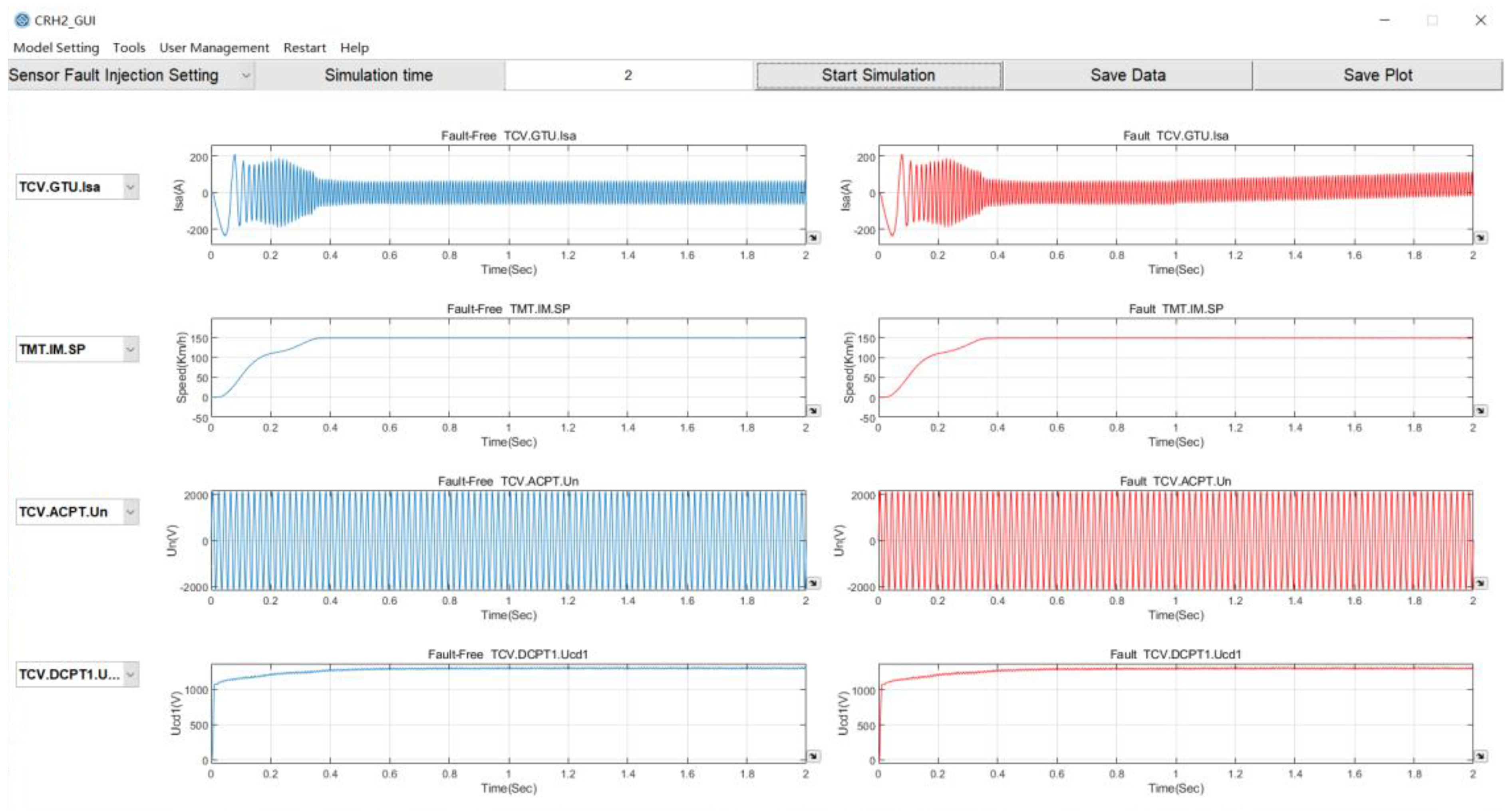
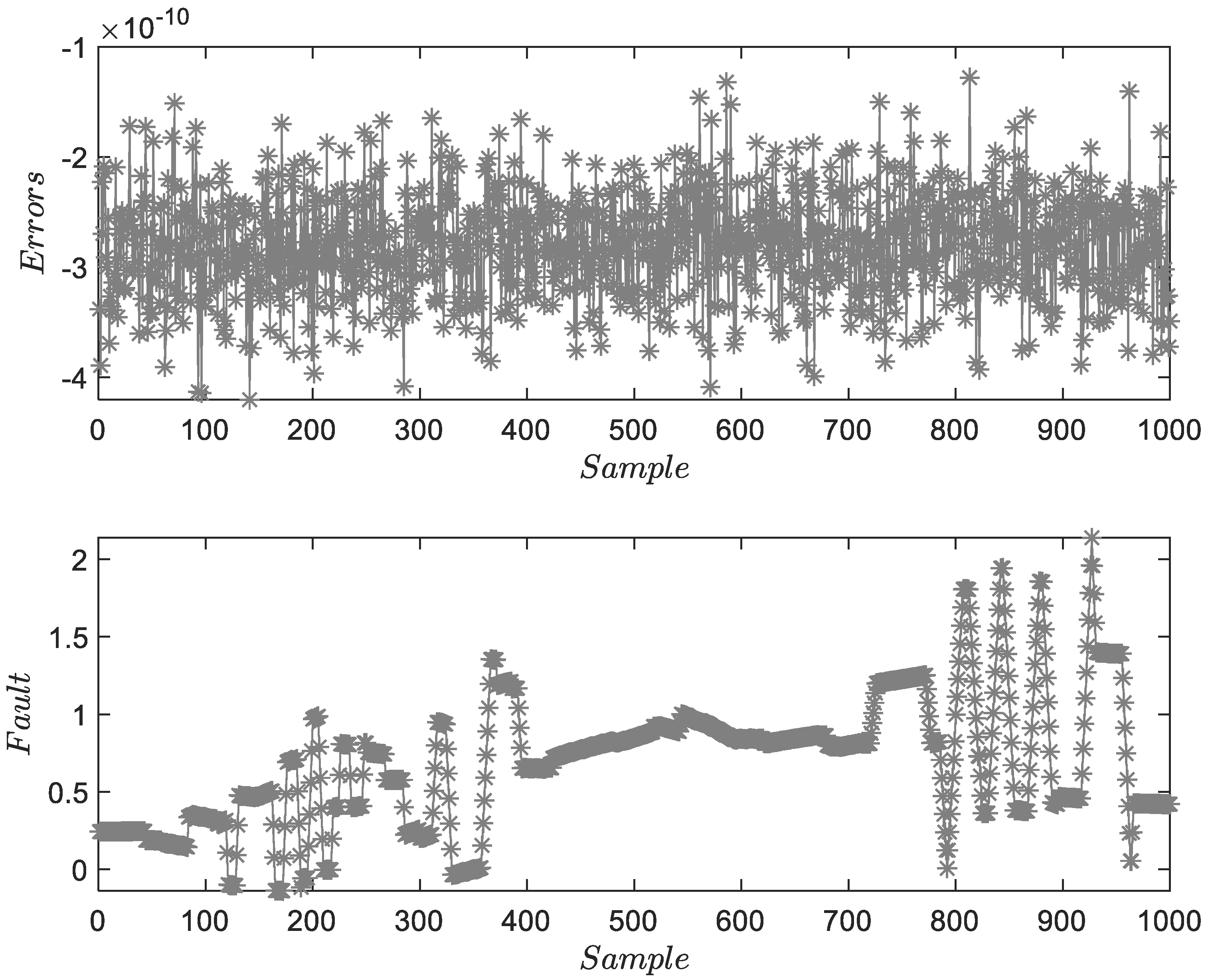
4.1. Experiment on a Traction Drive Control Numerical Platform

This part introduces a simulation platform that is shown in Figure 2. The fault injection is accomplished for verification. Three kinds of faults are injected, consisting of offset faults, drift faults, and stuck faults, respectively.

(1)

Fault 1: $f_1$ is an offset fault, which manifested by a constant between the measurements and real values. It can be caused by errors of sensors or environmental factors. This constant does not change over time. The fault parameter of injection is 5.

(2)

Fault 2: $f_2$ is a drift fault. The main manifestation of $f_2$ is that the measurement error varies over time. The environment, structure of sensors, and external disturbances can all lead to drift faults, affecting the long-term stability and accuracy of the sensor. The fault parameter of injection is (120,20).

(3)

Fault 3: $f_3$ is a gain fault, which commonly occurs in systems. The wear of mechanical equipment is the main reason for this fault. The fault parameter of injection is 5.

Figure 3, Figure 4 and Figure 5 show the FD and FE results for $f_1$, $f_2$, and $f_3$, respectively. The horizontal coordinate is the sample, and the unit is the sample ordinal number. The ordinate is the same unit as the system output in volts.

Figure 3 shows the FD and FE results for $f_1$. The upper subfigure proves the accuracy of system identification. The lower subfigure can illustrate the residuals of FD and obtain the accuracy estimations of $f_1$. Figure 4 and Figure 5 show the FD and FE results for $f_2$ and $f_3$. Two figures describe the characteristics of fixed-amplitude faults. Due to the existence of process and measurement noises, the estimation results fluctuate locally. Considering that the amplitude of the fault is much larger than the mean of random noise, the threshold will not be affected. However, under the assumption of colored noise, the threshold needs to be re-optimized.

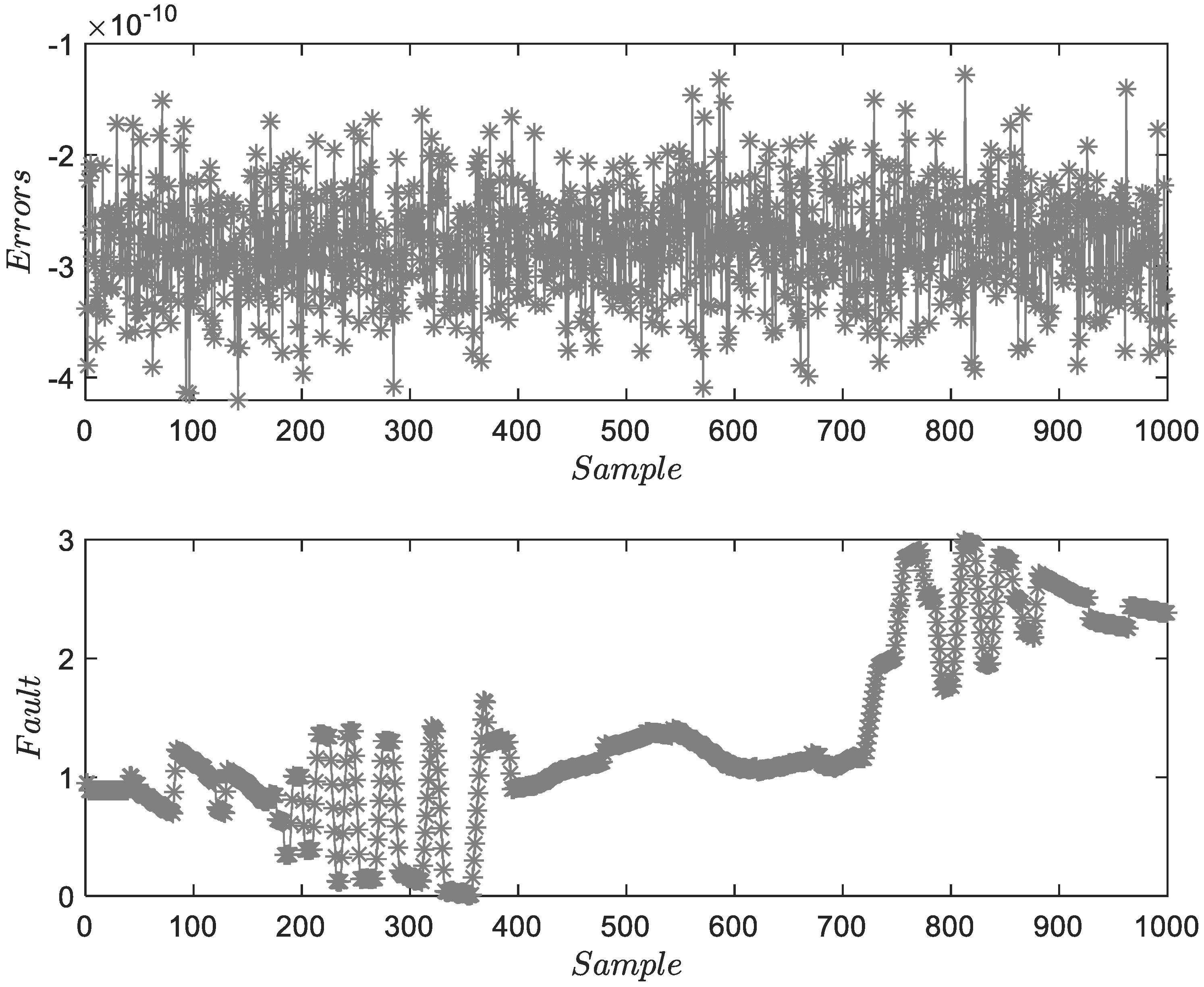
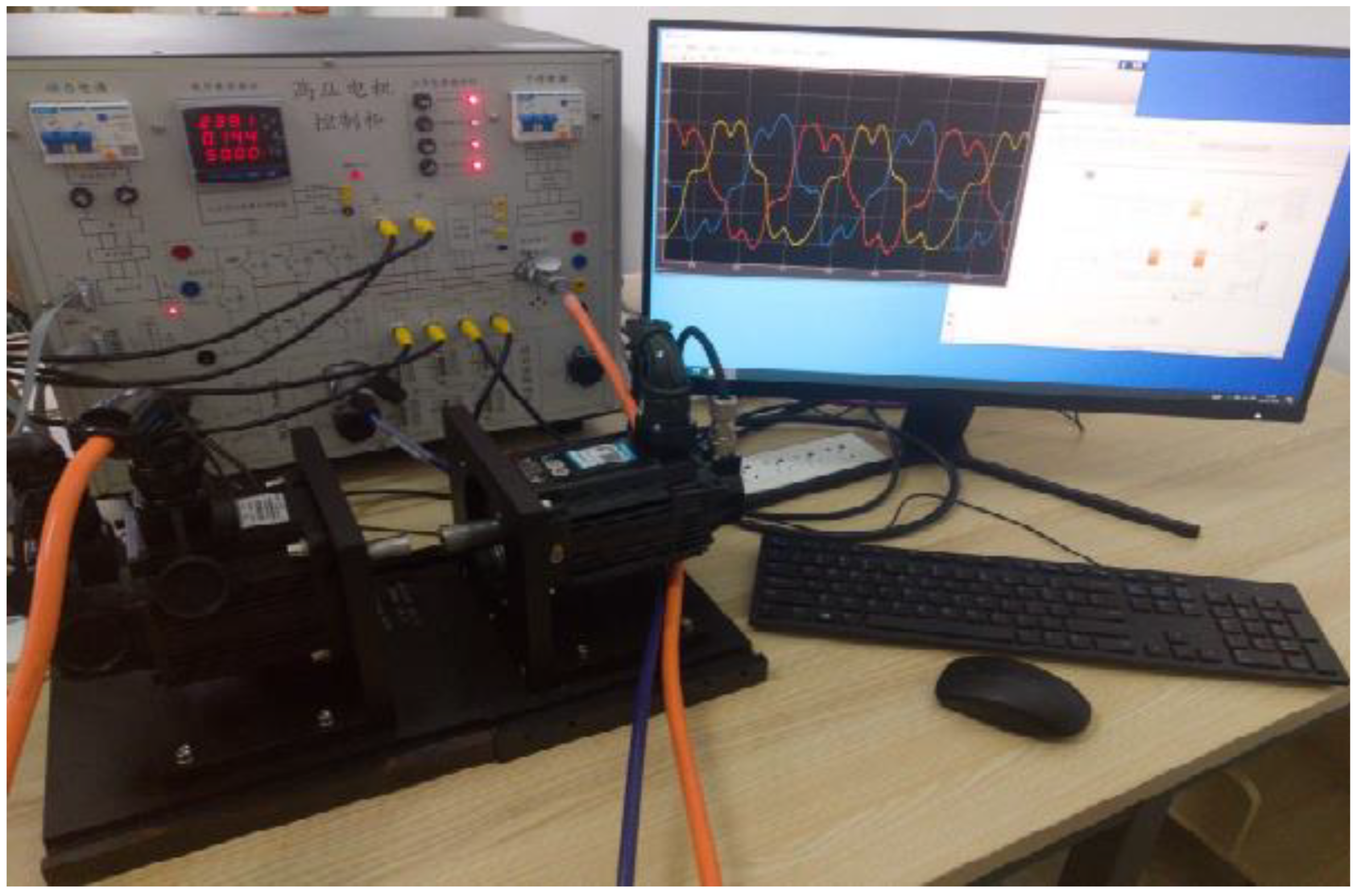
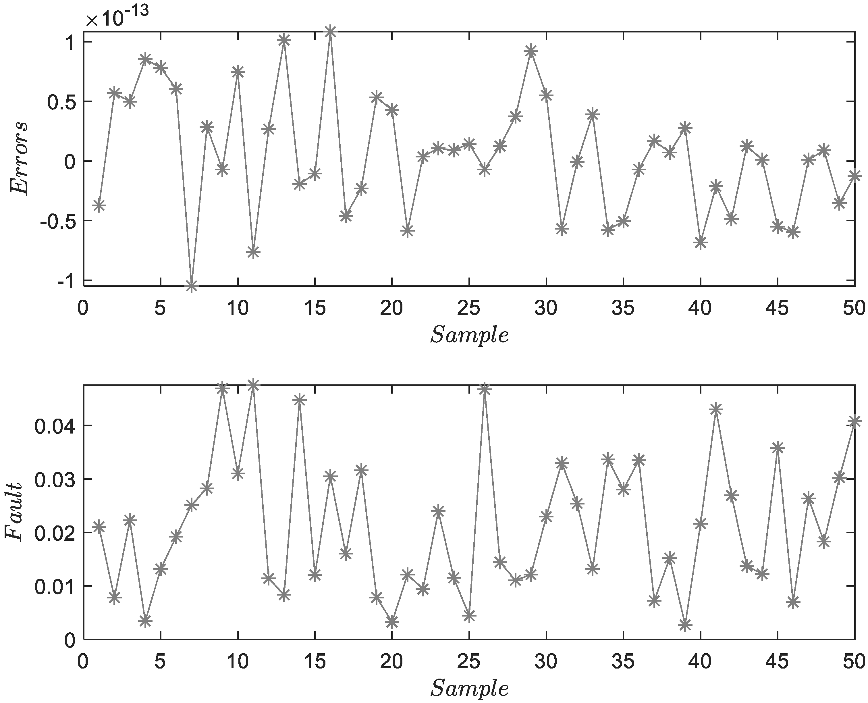
4.2. Experiment on a Pilot-Scale Traction Motor Platform

To further prove the effectiveness and practicability of this method, a pilot-scale traction motor platform is considered in this part. The specific structure of this platform is shown in Figure 6. Three faults with different amplitudes are given in this experiment, as follows.

(1)

Fault 4: $f_4$ is a sensor fault with a fault amplitude of 0.025.

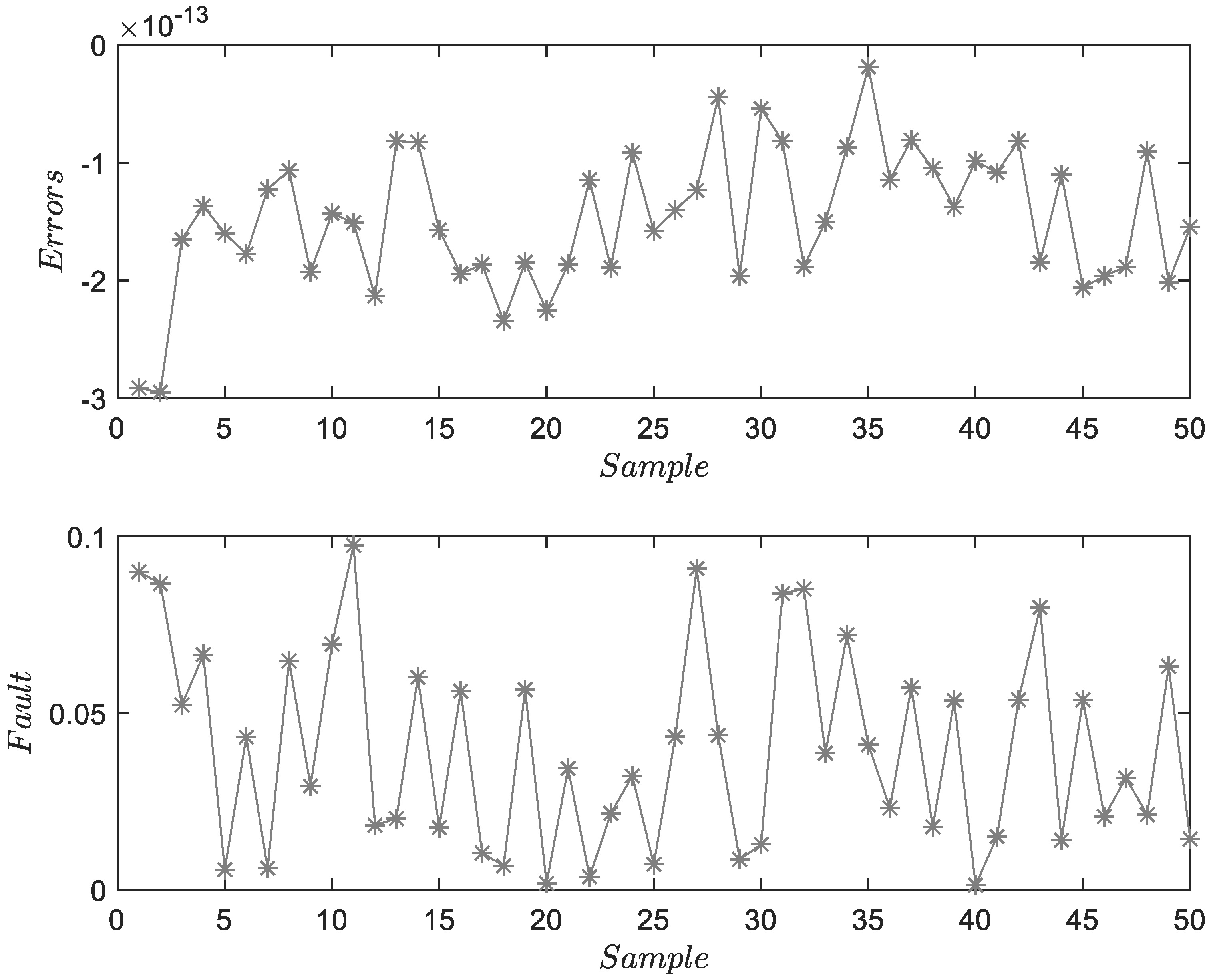
(2)

Fault 5: $f_5$ is a sensor fault with a fault amplitude of 0.05.

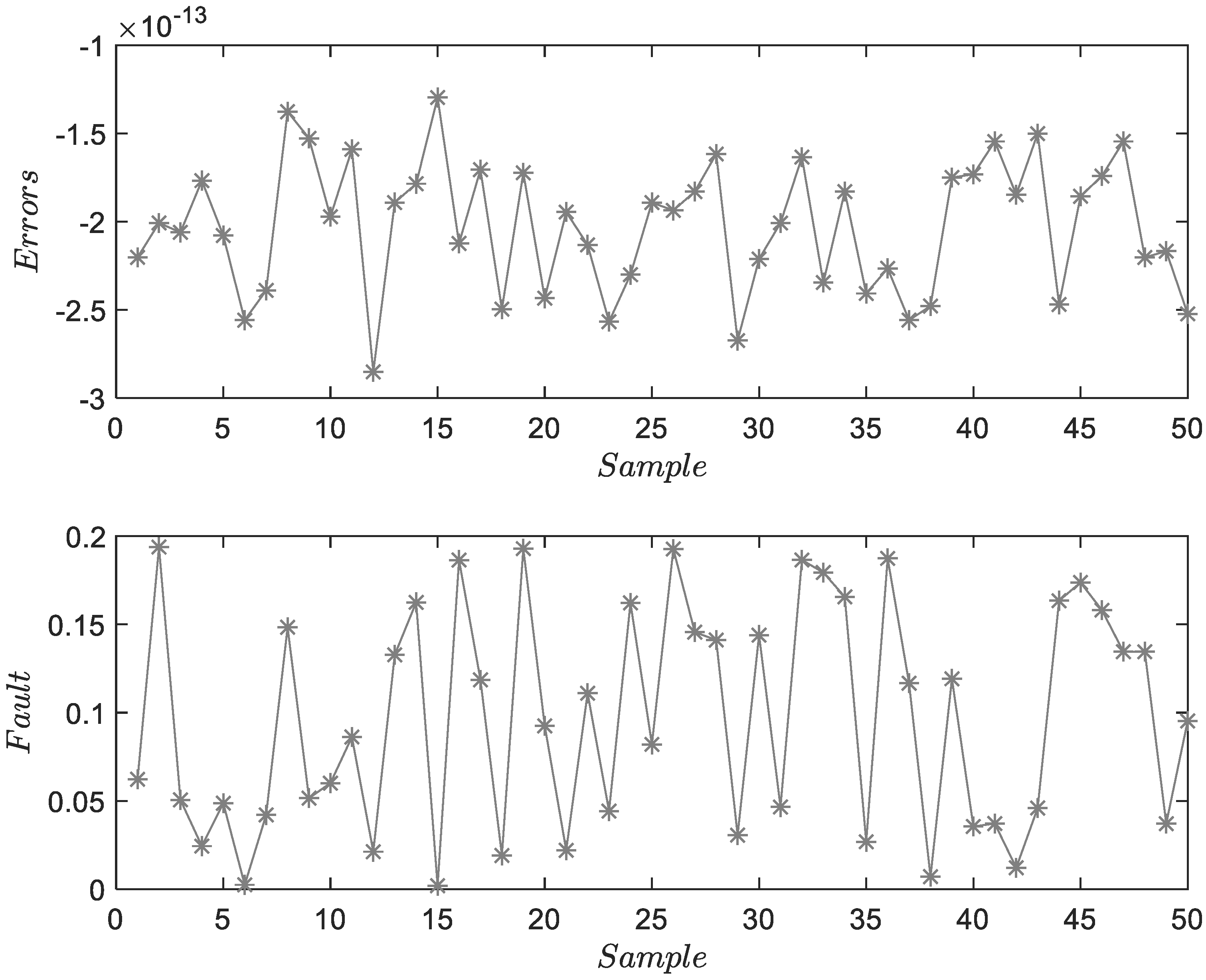
(3)

Fault 6: $f_6$ is a sensor fault with a fault amplitude of 0.1.

The results show the effectiveness of the proposed method for traction systems on a laboratory platform. The horizontal coordinate is the sample, and the unit is the sample ordinal number. The ordinate is the same unit as the system output in amperes. The subfigures in Figure 7, Figure 8 and Figure 9 are errors of the identification of the model and the estimated faults, respectively. In these figures, the errors of system identification are less than $1\times {10}^{-12}$, showing that the proposed method can adequately describe the system dynamics. The estimated results obtained by this method are the same as in the case of fault injection, which shows that FD and FE can be accurately realized in the given 50 samples. Because the current data obtained by the motor are periodic, 50 samples collected in a cycle range are sufficient to prove the effectiveness and practicability of the method.

4.3. Discussion

To further verify the superiority of the proposed method, this study provides a comparison of experiments in this section. The results of the comparison of experiments are shown in

Table 1. Comparison results.

Methods	MSE1	MSE2	MSE3	Time Consumption
DSFA	−5.84 $\times {10}^{-23}$	1.96 $\times {10}^{-23}$	53.57	1.85 s
CCA	1.12	1.98	1.87	1.42 s
FCNN	0.010	0.028	0.063	1.34 s
LSTM	0.202	0.364	0.252	6.90 s
The proposed method	4.12 $\times {10}^{-26}$	0.013	0.004	0.25 s

. Five different methods commonly used for FD and FE are selected in this experiment, encompassing deep slow feature analysis (DSFA), CCA, full-connection neural network (FCNN), long short-term memory (LSTM), and the proposed method. To obtain reliable results, the experimental settings of these methods are the same as those of the experiment in Section 4.2. The mean square error (MSE) and time consumption are selected to evaluate the results of the methods. In Table 1, MSE1 represents the MSE of FD for fault-free systems. MSE2 represents the MSE of FD for faulty systems. and MSE3 represents the MSE of FE for faulty systems.

Although missing data problems were studied so far, FD and FE methods using the state-space model for these problems in traction systems are still needed to be exploited. Therefore, starting from the state-space model and solving the missing data problems through the calculation of posterior probability ensures the dynamic performance of the algorithm and improves the repeatability of the Bayesian filtering method. The identification of the data-driven model via the data stacking technique is beneficial for providing an accuracy detection model for the traction systems of high-speed trains. Considering the characteristics of this method, some critical issues are necessary to state. Firstly, analyzing the parameter variation characteristics of the state-space model of a traction system can enhance the practicability of the theoretical method regarding its applications. Moreover, there are many causes of missing data problems, including hardware faults (sensors, communication devices, storage devices), software faults (software vulnerabilities), network faults (network congestion, network interference), and human causes (improper operation, improper maintenance). Lastly, nonlinear characteristics are common in practical systems, and the nonlinear extension of data-driven methods is an important problem worthy of further study.

5. Conclusions

Time series data are a critical element for analyzing the operating status of industrial power systems. The accuracy of FD and FE is affected by data quality. This study designed an MP-based data generation method to tackle FD and FE tasks for electrical systems of industry. It is applicable to complex dynamic systems with missing data problems. Then, the data-driven FD and FE methods are constructed based on the subspace identification technique. The matrix decomposition method can ensure the optimal results under the premise of linear systems. The effectiveness and superiority of the proposed method can be verified by actual industrial process. From the experiments, the error of system identification is less than $1\times {10}^{-12}$, and the different types of faults can be estimated. The results are satisfactory. Since the core of the method proposed in this paper is Bayesian estimation, it is important for data-driven Kalman filtering. Subsequent studies can further analyze the mechanism of missing data problems, consider the complex distribution of data, and study feasible data-driven solutions. In addition, this method can also be considered to nonlinear systems, time-varying systems, and distributed systems.

References

1. Gao, Z.; Cecati, C.; Ding, S. A Survey of Fault Diagnosis and Fault-Tolerant Techniques—Part I: Fault Diagnosis with Model-Based and Signal-Based Approaches. IEEE Trans. Ind. Electron. 2015, 62, 3757–3767. [Google Scholar] [CrossRef]
2. Edwards, C.; Simani, S. Fault Diagnosis and Fault-Tolerant Control in Aerospace Systems. Int. J. Robust Nonlinear Control 2019, 29, 5291–5292. [Google Scholar] [CrossRef]
3. Chen, H.; Sun, W.; Zhang, W.; Jiang, B.; Ding, S.; Huang, B. Explainable Fault Diagnosis Using Invertible Neural Networks-Part I: A Left Manifold-based Solution. IEEE Trans. Neural Networks Learn. Syst. 2024. [Google Scholar] [CrossRef]
4. He, J.; Ouyang, M.; Chen, Z.; Chen, D.; Liu, S. A Deep Transfer Learning Fault Diagnosis Method Based on WGAN and Minimum Singular Value for Non-Homologous Bearing. IEEE Trans. Instrum. Meas. 2022, 71, 3509109. [Google Scholar] [CrossRef]
5. Schmid, M.; Gebauer, E.; Hanzl, C.; Endisch, C. Active Model-Based Fault Diagnosis in Reconfigurable Battery Systems. IEEE Trans. Power Electron. 2021, 36, 2584–2597. [Google Scholar] [CrossRef]
6. Chen, H.; Luo, H.; Huang, B.; Jiang, B.; Kaynak, O. Transfer Learning-motivated Intelligent Fault Diagnosis Designs: A Survey, Insights, and Perspectives. IEEE Trans. Neural Networks Learn. Syst. 2024, 35, 2969–2983. [Google Scholar] [CrossRef]
7. Li, D. Robust Fault Detection and Estimation Observer Design for Switch Systems. Nonlinear Anal. Hybrid Syst 2019, 34, 30–42. [Google Scholar] [CrossRef]
8. Cui, Z.; Hu, W.; Zhang, G.; Huang, Q.; Chen, Z.; Blaabjerg, F. A Novel Data-Driven Online Model Estimation Method for Renewable Energy Integrated Power Systems with Random Time Delay. IEEE Trans. Power Syst. 2023, 38, 5930–5933. [Google Scholar] [CrossRef]
9. Yu, M.; Wang, W.; Wang, Y. Closed-Loop Continuous-Time Subspace Identification with Prior Information. Mathematics 2023, 11, 4924. [Google Scholar] [CrossRef]
10. Chen, H.; Jiang, B.; Lu, N.; Mao, Z. Deep PCA Based Real-Time Incipient Fault Detection and Diagnosis Methodology for Electrical Drive in High-Speed Trains. IEEE Trans. Veh. Technol. 2018, 67, 4819–4830. [Google Scholar] [CrossRef]
11. Li, Z.; Pang, W.; Liang, H.; Chen, G.; Zheng, X.; Ni, P. Multicomponent Alkane IR Measurement System Based on Dynamic Adaptive Moving Window PLS. IEEE Trans. Instrum. Meas. 2022, 71, 7006313. [Google Scholar] [CrossRef]
12. Xiu, X.; Li, Y. Learning Sparse Kernel CCA with Graph Priors for Nonlinear Process Monitoring. IEEE Sens. J. 2023, 23, 7381–7389. [Google Scholar] [CrossRef]
13. Zhang, Y.; Han, B.; Han, M. A Novel Distributed Data-Driven Strategy for Fault Detection of Multi-Source Dynamic Systems. IEEE Trans. Circuits Syst. II Express Briefs 2022, 69, 4379–4383. [Google Scholar] [CrossRef]
14. Bi, P.; Du, X. Arbitrary Triangle Structure Adaptive Mean PCA and Image Recognition. IEEE Trans. Circuits Syst. Video Technol. 2024, 34, 754–769. [Google Scholar] [CrossRef]
15. Shah, M.; Ahmed, Z.; Lisheng, H. Weighted Linear Local Tangent Space Alignment via Geometrically Inspired Weighted PCA for Fault Detection. IEEE Trans. Ind. Inf. 2023, 19, 210–219. [Google Scholar] [CrossRef]
16. Zhang, C.; Dong, J.; Meng, S.; Cong, Z.; Peng, K. A Two-Layer Distributed Fault Diagnosis Method Based on Correlation Feature Transfer for Large-Scale Sequential Process Industries. IEEE Trans. Instrum. Meas. 2023, 73, 3501214. [Google Scholar] [CrossRef]
17. Rishi, M.; Tangirala, A. Probabilistic Adaptive Slow Feature Analysis for State Estimation and Classification. IEEE Trans. Instrum. Meas. 2024, 73, 1002515. [Google Scholar] [CrossRef]
18. Ding, S. Data-Driven Design of Monitoring and Diagnosis Systems for Dyanamic Processes: A Review of Subspace Technique Based Schemes and Some Recent Results. J. Process Control 2014, 24, 431–449. [Google Scholar] [CrossRef]
19. Huo, M.; Luo, H.; Cheng, C.; Li, K.; Yin, S.; Kaynak, O.; Zhang, J.; Tang, D. Subspace-Aided Sensor Fault Diagnosis and Compensation for Industrial Systems. IEEE Trans. Ind. Electron. 2023, 70, 9474–9482. [Google Scholar] [CrossRef]
20. Zhao, Z.; Xu, Y.; Li, Y.; Zhao, Y.; Wang, B.; Wen, G. Sparse Actuator Attack Detection and Identification: A Data-Driven Approach. IEEE Trans. Cybern. 2023, 53, 4054–4064. [Google Scholar] [CrossRef]
21. Yu, M.; Wang, Y.; Wang, W.; Wei, Y. Continuous-Time Subspace Identification with Prior Information Using Generalized Orthonormal Basis Functions. Mathematics 2023, 11, 4765. [Google Scholar] [CrossRef]
22. Yin, S.; Gao, H.; Qiu, J.; Kaynak, O. Fault Detection for Nonlinear Process with Deterministic Disturbances: A Just-In-Time Learning Based Data Driven Method. IEEE Trans. Cybern. 2017, 47, 3649–3657. [Google Scholar] [CrossRef] [PubMed]
23. Chen, Z.; Ding, S.; Luo, H.; Zhang, K. An Alternative Data-Driven Fault Detection Scheme for Dyanmic Processes with Deterministic Disturbances. J. Franklin Inst. 2017, 354, 556–570. [Google Scholar] [CrossRef]
24. Luo, H.; Yin, S.; Kayank, O. A Data-Driven Fault Detection Approach for Dynamic Processes with Sinusoidal Disturbance. In Proceedings of the IEEE International Conference on Systems, Man, and Cybernetics, Miyazaki, Japan, 7–10 October 2018. [Google Scholar]
25. Xu, S. Disturbance Observer-Based Adaptive Fault Tolerant Control with Prescribed Performance of a Continuum Robot. Actuators 2024, 13, 267. [Google Scholar] [CrossRef]
26. Li, L.; Ding, S.; Peng, X. Optimal Observer-Based Fault Detection and Estimation Approaches for T–S Fuzzy Systems. IEEE Trans. Fuzzy Syst. 2022, 30, 579–590. [Google Scholar] [CrossRef]
27. Liang, D.; He, Z.; Ding, S.; Yang, Y. Distributed Fault Estimation and Fault-Tolerant Control of Interconnected Systems with Plug-and-Play Features. IEEE Trans. Circuits Syst. I Regul. Pap. 2024, 71, 431–442. [Google Scholar] [CrossRef]
28. Hu, Y.; Dai, X.; Wu, Y.; Jiang, B.; Cui, D.; Jia, Z. Robust Fault Estimation and Fault-Tolerant Control for Discrete-Time Systems Subject to Periodic Disturbances. IEEE Trans. Circuits Syst. I Regul. Pap. 2023, 70, 2982–2994. [Google Scholar] [CrossRef]
29. Liang, Y.; Zhang, J.; Shi, Z.; Zhao, H.; Wang, Y.; Xing, Y.; Zhang, X.; Wang, Y.; Zhu, H. A Fault Identification Method of Hybrid HVDC System Based on Wavelet Packet Energy Spectrum and CNN. Electronics 2024, 13, 2788. [Google Scholar] [CrossRef]
30. Song, C.; Yang, Y. Nonlinear-Observer-Based Neural Fault-Tolerant Control for a Rehabilitation Exoskeleton Joint with Electro-Hydraulic Actuator and Error Constraint. Appl. Sci. 2023, 13, 8294. [Google Scholar] [CrossRef]
31. Cheng, C.; Wang, W.; Ran, G.; Chen, H. Data-Driven Designs of Fault Identification via Collaborative Deep Learning for Traction Systems in High-Speed Trains. IEEE Trans. Transp. Electrif. 2022, 8, 1748–1757. [Google Scholar] [CrossRef]
32. Mu, D.; Lin, S.; Zhang, H.; Zheng, T. A Novel Fault Identification Method for HVDC Converter Station Section Based on Energy Relative Entropy. IEEE Trans. Instrum. Meas. 2022, 71, 3507910. [Google Scholar] [CrossRef]
33. Hassan, M.; Hossain, M.; Shah, R. DC Fault Identification in Multiterminal HVDC Systems Based on Reactor Voltage Gradient. IEEE Access 2021, 9, 115855–115867. [Google Scholar] [CrossRef]
34. Ma, G.; Zhang, H.; Sun, Z.; Yao, C.; Ren, G.; Xu, S. Current Sensor Fault Localization and Identification of PMSM Drives Using Difference Operator. IEEE J. Emerging Sel. Top. Power Electron. 2023, 11, 1097–1110. [Google Scholar] [CrossRef]
35. Yang, S.; Sun, X.; Ma, M.; Zhang, X.; Chang, L. Fault Detection and Identification Scheme for Dual-Inverter Fed OEWIM Drive. IEEE Trans. Ind. Electron. 2020, 67, 6112–6123. [Google Scholar] [CrossRef]
36. Wang, Z.; Han, C.; Gao, H.; Guo, F. Identification of Series Arc Fault Occurred in the Three-Phase Motor with Frequency Converter Load Circuit via VMD and Entropy-Based Features. IEEE Sens. J. 2022, 22, 24320–24332. [Google Scholar] [CrossRef]
37. Wang, Q.; Zhao, X.; Yang, P.; Hua, W.; Buja, G. Effects of Triangular Wave Injection and Current Differential Terms on Multiparameter Identification for PMSM. IEEE Trans. Power Electron. 2024, 39, 2943–2947. [Google Scholar] [CrossRef]
38. Zhang, Z.; Ren, J.; Tang, X.; Jing, S.; Lee, W. Novel Approach for Arc Fault Identification with Transient and Steady State Based Time-Frequency Analysis. IEEE Trans. Ind. Appl. 2022, 58, 4359–4369. [Google Scholar] [CrossRef]
39. Husari, F.; Seshadrinath, J. Early Stator Fault Detection and Condition Identification in Induction Motor Using Novel Deep Network. IEEE Trans. Artif. Intell. 2022, 3, 809–818. [Google Scholar] [CrossRef]
40. Langarica, S.; Ruffelmacher, C.; Nunez, F. An Industrial Internet Application for Real-Time Fault Diagnosis in Industrial Motors. IEEE Trans. Autom. Sci. Eng. 2020, 17, 284–295. [Google Scholar] [CrossRef]
41. Liu, Y.; Chen, Z.; Wei, L.; Wang, X.; Li, L. Braking Sensor and Actuator Fault Diagnosis with Combined Model-Based and Data-Driven Pressure Estimation Methods. IEEE Trans. Ind. Electron. 2023, 70, 11639–11648. [Google Scholar] [CrossRef]
42. Liu, P.; Zhang, Y.; Dai, Y.; Sun, Y. Arc Grounding Fault Identification Using Integrated Characteristics in the Power Grid. Energy Eng. 2024, 121, 1883–1901. [Google Scholar] [CrossRef]
43. Tian, J.; Zeng, G.; Zhao, J.; Zhu, X.; Zhang, Z. A Data-Driven Modeling Method of Virtual Synchronous Generator Based on LSTM Neural Network. IEEE Trans. Ind. Inf. 2024, 20, 5428–5439. [Google Scholar] [CrossRef]
44. Sun, W.; Shi, X.; Xiong, W.; Chen, H.; Huang, B. A Conditional Invertible Neural Network-based Fault Detection. TechRxiv 2024. [Google Scholar] [CrossRef]
45. Yu, H.; Zhang, G.; Wang, R.; Xiong, W. A Real-Time Adaptive Energy Optimization Method for Urban Rail Flexible Traction Power Supply System. IEEE Trans. Intell. Transp. Syst. 2023, 24, 10155–10164. [Google Scholar] [CrossRef]
46. Sameni, R.; Shamsollahi, M.; Jutten, C.; Clifford, G. A Nonlinear Bayesian Filtering Framework for ECG Denoising. IEEE Trans. Biomed. Eng. 2007, 54, 2172–2185. [Google Scholar] [CrossRef]
47. Liu, X.; Liu, X.; Yang, Y.; Guo, Y.; Zhang, W. Variational Bayesian-Based Robust Cubature Kalman Filter with Application on SINS/GPS Integrated Navigation System. IEEE Sens. J. 2022, 22, 489–500. [Google Scholar] [CrossRef]
48. Liu, J.; Wang, Z.; Cheng, D.; Chen, W.; Chen, C. Marine Extended Target Tracking for Scanning Radar Data Using Correlation Filter and Bayes Filter Jointly. Remote Sens. 2022, 14, 5937. [Google Scholar] [CrossRef]
49. Brouillon, J.; Fabbiani, E.; Nahata, P.; Moffat, K.; Dorfler, F.; Trecate, G. Bayesian Error-in-Variables Models for the Identification of Distribution Grids. IEEE Trans. Smart Grid 2023, 14, 1289–1299. [Google Scholar] [CrossRef]
50. Fong, E.; Lyddon, S.; Holmes, C. Scalable Nonparametric Sampling from Multimodal Posteriors with the Posterior Bootstrap. In Proceedings of the 36th International Conference on Machine Learning, Online, 9 June 2019. [Google Scholar]
51. Wu, L.; Williamson, S. Posterior Uncertainty Quantification in Neural Networks using Data Augmentation. In Proceedings of the 27th International Conference on Artificial Intelligence and Statistics, Valencia, Spain, 2 May 2024. [Google Scholar]
52. Yang, X.; Yang, C.; Peng, T.; Chen, Z.; Liu, B.; Gui, W. Hardware-in-the-Loop Fault Injection for Traction Control System. IEEE J. Emerging Sel. Top. Power Electron. 2018, 6, 696–706. [Google Scholar] [CrossRef]
Figure 1. Overall process of data generation and data-driven modeling.
Mathematics 12 03200 g001
Figure 2. Fault injection benchmark for traction drive control system.
Mathematics 12 03200 g002
Figure 3. Result of FD and FE for f 1 .
Mathematics 12 03200 g003
Figure 4. Result of FD and FE for f 2 .
Mathematics 12 03200 g004
Figure 5. Result of FD and FE for f 3 .
Mathematics 12 03200 g005
Figure 6. Pilot-scale traction motor platform.
Mathematics 12 03200 g006
Figure 7. Result of FD and FE for f 4 .
Mathematics 12 03200 g007
Figure 8. Result of FD and FE for f 5 .
Mathematics 12 03200 g008
Figure 9. Result of FD and FE for f 6 .
Mathematics 12 03200 g009