Article

Composite and Mixture Distributions for Heavy-Tailed Data—An Application to Insurance Claims

by
Walena Anesu Marambakuyana
and
Sandile Charles Shongwe
*
Department of Mathematical Statistics and Actuarial Science, Faculty of Natural and Agricultural Sciences, University of the Free State, Bloemfontein 9301, South Africa
*
Author to whom correspondence should be addressed.
Mathematics 2024, 12(2), 335; https://doi.org/10.3390/math12020335
Submission received: 21 December 2023 / Revised: 18 January 2024 / Accepted: 18 January 2024 / Published: 19 January 2024

Abstract

:
This research provides a comprehensive analysis of two-component non-Gaussian composite models and mixture models for insurance claims data. These models have gained attraction in actuarial literature because they provide flexible methods for curve-fitting. We consider 256 composite models and 256 mixture models derived from 16 popular parametric distributions. The composite models are developed by piecing together two distributions at a threshold value, while the mixture models are developed as convex combinations of two distributions on the same domain. Two real insurance datasets from different industries are considered. Model selection criteria and risk metrics of the top 20 models in each category (composite/mixture) are provided by using the ‘single-best model’ approach. Finally, for each of the datasets, composite models seem to provide better risk estimates.

1. Introduction

In the area of loss modelling, basic classical distributions such as the lognormal, Weibull, gamma, Pareto, and Burr distributions are increasingly becoming less popular as composite and mixture models are gaining more attention because of their flexibility. Composite models are developed by piecing together two distributions (which are termed head and tail distributions) at a threshold value so that small and moderate losses are modelled by the head distribution, whereas large losses are modelled by the tail distribution. On the other hand, mixture models are developed as convex combinations of distributions defined on the same overlapping domain, i.e., the positive real line. The different combinations of models that can be constructed provide a large degree of flexibility for modelling heavy-tailed loss data.
The first composite model used to model actuarial data was proposed by Cooray and Ananda [1]. This model has paved the way for more composite model research in the actuarial and risk management curriculum. The idea behind the model was to use the lognormal distribution to model the behaviour of small and moderate losses (high frequency/low severity) and the Pareto distribution to model the behaviour of the large losses (low frequency/high severity). However, this model was criticised by Scollnik [2] as it can be interpreted as a two-component mixture model with fixed and a priori known mixing weights. Scollnik [2] then proposed two models with unrestricted mixing weights. Unlike the model proposed by [1], these models provided more flexibility due to the accommodation of different proportions of the two distributions of the composite model. The models discussed in Scollnik [2] were extended by Pigeon and Denuit [3] for when the threshold is assumed to vary among observations. Pigeon and Denuit [3] proposed two examples of distributions which can be used for the threshold—this resulted in the gamma-distributed threshold and lognormaldistributed threshold. Next, Nadarajah and Bakar [4] introduced the composite lognormal-Burr model, where it was observed that in the case of the Danish fire loss data, this model performed better than the composite lognormal-Pareto family. Parallel to the studies based on the composite lognormal models at that time, Ciumara [5] introduced a model with the Weibull distribution to model the behaviour of small and moderate losses and the Pareto distribution to model the behaviour of large losses. Scollnik and Sun [6] also criticised the restrictive nature of the fixed and a priori known mixing weights of the model discussed in Ciumara [5]. Scollnik and Sun [6] proposed two additional models with unrestricted weights. Abu Bakar et al. [7] extended the class of Weibull composite distributions by proposing seven models with the tail belonging to the family of transformed beta distributions. The new composite models proposed were the composite Weibull-Burr, the composite Weibull-Loglogistic, the composite Weibull-Paralogistic, the composite Weibull-Generalised Pareto, the composite Weibull-Inverse Burr, the composite Weibull-Inverse Pareto and the composite Weibull-Inverse paralogistic models. At the time of their study, [7] found that the composite models with the Weibull as the head distribution performed better for the Danish fire loss data compared to other composite models in the literature. The extension of the framework for composite models was provided by Grün and Miljkovic [8], where they conducted a thorough analysis of 256 distinct composite curve-fitting models which emerged from piecing together two distributions (i.e., head and tail distributions) from the list of 16 widely used parametric distributions—these are provided in Table A1 in Appendix A.
For the Danish fire loss data, Grün and Miljkovic [8] identified the top 20 composite models that fit the data the best and examined the goodness-of-fit characteristics and risk assessments for those 20 models. The composite Weibull-Inverse Weibull, composite Paralogistic-Inverse Weibull, and composite Inverse Burr-Inverse Weibull, respectively, were the top three models based on the Bayesian Information Criterion (BIC). Among the 256 composite models assessed, none of the top 20 best-fitting had the lognormal distribution in the head. Contrarily, using the Weibull, paralogistic, and inverse Burr distributions in the head was proven to be the most practical approach for simulating the small- and moderate-sized claims of Danish fire loss data. The best choices for modelling the long tail of the loss data were the inverse Weibull, inverse paralogistic, loglogistic, Burr, inverse gamma, and paralogistic. Neither the Pareto nor the generalised Pareto distributions were among the top 20 based on the BIC. Calderin-Ojeda and Kwok [9] suggested the use of composite models where the mode is the splice point (or the truncation point). This method is known as the mode matching procedure, and it was used to construct the composite lognormal-Stoppa and the composite Weibull-Stoppa, where the composite Weibull-Stoppa model had the best performance up to date for the Danish data.
Keatinge [10] introduced the use of the mixture of exponentials as a semiparametric approach. Klugman and Rioux [11] stated that a drawback of the mixture of exponentials is its zero mode, and they proposed the augmented mixture of exponentials distribution which consisted of the mixture of exponentials, the gamma or lognormal distribution, and the Pareto distribution, respectively. Lee and Lin [12] stated that a drawback of the augmented mixture of exponentials is that it has a maximum of three modes, and they proposed a mixture of Erlang distributions with the same scale parameter. It is said that the mixture of Erlang distributions is dense in the space of positive, continuous distributions (Tijms, [13]). Lee and Lin [12] also demonstrated that a uniform distribution, a mixture of two gamma distributions, a generalised Pareto distribution, and the lognormal distribution can be approximated by a mixture of Erlang distributions. Finally, Lee and Lin [12] fitted the mixture of Erlang distributions to the US catastrophic loss data. Miljkovic and Grün [14] stated that a drawback of using the mixture of Erlangs with the same scale parameter could be that more components may be required to obtain an adequate fit that could have otherwise been attained without this restriction. Next, Miljkovic and Grün [14] proposed mixtures of non-Gaussian distributions with no restrictions on the parameters. Their best three models for the Danish data based on minimum BIC were the two-component Burr mixture, the three-component inverse Burr mixture, and the five-component lognormal mixture. In addition, Miljkovic and Grün [14] further added that these three models have lower negative log-likelihood (NLL), Akaike Information Criterion (AIC), and BIC in comparison to the composite Weibull-Burr, composite Weibull-Loglogistic, and the Weibull-Inverse paralogistic distributions which were considered to be the best three composite models in [7]. Abu Bakar et al. [15] proposed six two-component mixture models for fitting three real datasets—the Danish, AON Re Belgium, and Norwegian fire loss datasets. The two-component Burr mixture and the two-component lognormal were the first- and second-best models for the three datasets, respectively. However, the two-component exponential mixture was the worst for the Belgian and Danish fire loss datasets, while the two-component Pareto mixture was the worst for the Norwegian fire loss data. Abu Bakar and Nadarajah [16] proposed two-component mixture models based on the inverse transformed gamma and the transformed beta families, where their fit was illustrated using the Danish fire loss data. Furthermore, Abu Bakar and Nadarajah [16] stated that these families are appropriate for modelling loss data because of the high degree of skewness present in the tails of the distributions. This resulted in seventeen two-component mixtures, all with the inverse transformed gamma as the first component distribution and they found that these models have a better fit for the Danish data based on the BIC than all the composite models and mixture models that had been considered for the Danish dataset in the past.
In the spirit of modelling insurance claims data, many other authors have studied loss distributions. Asgharzadeh et al. [17] introduced the generalised inverse Lindley distribution for the Danish data and found it to be better than most of the classical heavy-tailed distributions, but not as good as the composite models. Next, Punzo et al. [18] introduced nine compound models using three real-life datasets (namely, the US indemnity losses, automobile insurance claims, and Norwegian fire claims). These models were said to have more flexibility than the unimodal two-parameter lognormal, inverse Gaussian, and gamma distributions due to the additional parameters. Bhati and Ravi [19] proposed the use of the generalised log-Moyal distribution and fitted it to the Danish and Norwegian fire loss datasets. Motivated by the research work of [18,19], Li et al. [20] proposed the use of the three-parameter gamma mixture of the generalised log-Moyal distribution, and it was shown to be a special case of the four-parameter generalised beta of the second kind. Zhao et al. [21] and Ahmad et al. [22] introduced additional new heavy-tailed distributions for use in insurance data analysis. While the above review is by no means comprehensive, it provides an overall view of the current literature for heavy-tailed (insurance/claims) data analysis.
This paper is motivated by the recent work by: (i) Grün and Miljkovic [8] where 256 composite models were evaluated for the Danish fire loss data (note though, the corresponding 256 mixture models have not all been considered before); and (ii) Maphalla et al. [23] where the standard loss distributions with the best goodness of fit for the South African taxi claims data were found to be the lognormal and the Pareto, and the potential future research idea of modelling the South African taxi claims data using mixture models were suggested. One should note that due to the flexibility of two-component composite and mixture models, overfitting may easily occur. Thus, care needs to be exercised when fitting these models, especially when using mixture models with more than two components, as this may easily lead to overfitting and greatly violate the principle of parsimony.
In this paper, we consider a thorough comparison of 256 composite models and 256 mixture models for curve-fitting which are derived from 16 popular parametric distributions listed in Table A1 in Appendix A. This study focuses on the following objectives: (i) To discover composite models that have not been studied previously for the South African taxi claims data; (ii) To discover mixture models that have not been studied previously for the South African taxi claims data and Danish fire loss data; and (iii) To assess the implications of the different composite models and mixture models using risk measures, such as Value-at-Risk (VaR) and Tail Value-at-Risk (TVaR).
This paper is structured as follows: Section 2 provides the methodology, which includes model specification, risk measures, and model selection criteria. Section 3 provides the analysis, wherein all the results for the top 20 composite models and mixture models that yield the best goodness-of-fit to the Danish fire loss data and the South African taxi claims data are discussed. Different information criteria and risk measures are computed and presented for models studied in this paper, with additional results provided in Appendix A. Finally, Section 4 provides the concluding remarks.

2. Methodology

2.1. The Composite Model

2.1.1. Model Specification

The probability density function (pdf) of a composite model which was introduced in [7] and adapted by [8] is given by
f ϑ 1 , ϑ 2 , θ , ϕ = 1 1 + ϕ f 1 * x | ϑ 1 , θ , i f   0 < x θ ,   ϕ 1 + ϕ f 2 * x | ϑ 2 , θ , i f   θ < x < .
The continuity condition and the differentiability conditions are imposed at the threshold θ such that,
f ϑ 1 , ϑ 2 , θ , ϕ   = f ϑ 1 , ϑ 2 , θ , ϕ
f ϑ 1 , ϑ 2 , θ , ϕ = f ϑ 1 , ϑ 2 , θ , ϕ
where ϑ 1 and ϑ 2 are the parameter sets associated with the pdfs on the disjoint intervals, ( 0 ,   θ ] and θ ,   , respectively. The continuity and differentiability conditions ensure that the threshold parameter θ and the weight parameter ϕ > 0 are defined as functions of the other parameters, ϑ 1   and ϑ 2 . In addition, 1 1 + ϕ and ϕ 1 + ϕ are referred to as mixing weights, see [4]. Moreover, the continuity condition at threshold θ ensures that the weight parameter ϕ is expressed as a function of the other parameters ϑ 1 ,   ϑ 2 ,   θ , and cumulative distribution function (cdf) in closed form as,
ϕ = d ln F 1 θ | ϑ 1   d θ d ln 1 F 2 θ | ϑ 2   d θ = f 1 θ | ϑ 1 F 1 θ | ϑ 1 f 2 x | ϑ 2 1 F 2 θ | ϑ 2 .
Substituting the expression for ϕ obtained in Equation (4) into the differentiability condition in Equation (3) gives the following condition for the threshold θ , which simplifies to,
d d θ ln f 1 θ | ϑ 1 f 2 θ | ϑ 2 = 0 f 1 θ | ϑ 1 f 1 θ | ϑ 1 = f 2 θ | ϑ 2 f 2 θ | ϑ 2 .
Lastly, f 1 * x | ϑ 1 ,   θ   and f 2 * x | ϑ 2 ,   θ are truncated pdfs which are defined in terms of their corresponding pdfs and cdfs are
f 1 * x | ϑ 1 , θ = f 1 x | ϑ 1 F 1 θ | ϑ 1 ,
f 2 * x | ϑ 2 , θ = f 2 x | ϑ 2 1 F 2 θ | ϑ 2 ,
and also,
F ϑ 1 ,   ϑ 2 , θ , ϕ = 1 1 + ϕ F 1 x | ϑ 1 F 1 θ | ϑ 1 , i f   0 < x θ , 1 1 + ϕ 1 + ϕ F 2 x | ϑ 2 F 2 θ | ϑ 2 1 F 2 x | ϑ 2 , i f   θ < x < .  
The k th raw moment of the composite model is given in Grün and Miljkovic [8] as
E X k = 1 1 + ϕ E X 1 k F 1 k θ | ϑ 1 F 1 θ | ϑ 1 + ϕ 1 + ϕ E X 2 k 1 F 2 k θ | ϑ 2 1 F 2 θ | ϑ 2 ,
where X i is the random variable associated with the i th component and F i k is the k th incomplete moment distribution of the i th component distribution. For a random sample x = x 1 ,   x 2 ,   ,   x n , the log-likelihood function which was introduced in Grün and Miljkovic [8] is given by
l ϑ 1 , ϑ 2 | x = i = 1 n ln f x i | ϑ 1 , ϑ 2 .

2.1.2. Risk Measures

Abu Bakar et al. [7] and Grün and Miljkovic [8] defined the theoretical estimate for the VaR of X as
V a R p X = F 1 1 p 1 + ϕ F 1 θ , i f   0 < p 1 1 + ϕ , F 2 1 F 2 θ + p 1 + ϕ 1 1 F 2 θ / ϕ , i f   1 1 + ϕ < p < 1 .  
The theoretical estimates for the TVaR of X are defined in [8] as
T V a R p X = 1 1 p π p θ x f 1 x d x F 1 θ + θ x f 2 x d x 1 F 2 θ , i f   0 < p 1 1 + ϕ , 1 1 p 1 1 F 2 θ π p x f 2 x d x , i f   1 1 + ϕ < p < 1 .
Finite values of Equation (12) can only be obtained if the first moment of the tail distribution exists (Grün and Miljkovic, [8]).

2.2. The Mixture Model

2.2.1. Model Specification

The pdf of a two-component mixture model is given by
f x | ϑ 1 ,   ϑ 2 ,   ϕ = 1 1 + ϕ f 1 x | ϑ 1 + ϕ 1 + ϕ f 2 x | ϑ 2 , x > 0 ,
where ϕ > 0 is the weight parameter, and ϑ 1 and ϑ 2 are the parameter sets associated with the first and second component distributions, respectively, where f 1 and f 2 are the corresponding pdfs. The component distributions are both defined on R + . Therefore, the set of parameters of the mixture model is ϕ , ϑ 1 , ϑ 2 . Unlike the composite model, the weight parameter, ϕ , is not a function of the other parameters. Rather, the weight parameter is also a model parameter, which is estimated by the maximum likelihood method in a similar fashion as the other model parameters. The coefficients of f 1 and f 2 are called mixing weights and for ϕ > 0 , it is clear that 1 1 + ϕ + ϕ 1 + ϕ = 1 . For ϕ = 1 , the component distributions have equal mixing weights of 0.5, i.e., 1 1 + ϕ = ϕ 1 + ϕ = 0.5 . For ϕ < 1 , the first component distribution has a greater weight to the mixture model than the second component distribution. For ϕ > 1 , the second component distribution has a greater weight to the mixture model than the first component distribution.
The corresponding cdf is given by
F x | ϑ 1 ,   ϑ 2 ,   ϕ = 1 1 + ϕ F 1 x | ϑ 1 + ϕ 1 + ϕ F 2 x | ϑ 2 , x > 0 ,
where F 1 and F 2 are the cdfs of the first and second components, respectively. The kth raw moment of a two-component mixture model is given by
E X k = 1 1 + ϕ E X 1 k + ϕ 1 + ϕ E X 2 k , x > 0 ,
where E X 1 k and E X 2 k are the k th raw moments of the first and second components, respectively, given that they exist. The moment-generating function (mgf) of a two-component mixture model is given by
M X t = 1 1 + ϕ M X 1 t + ϕ 1 + ϕ M X 2 t ,
where M X 1 t and M X 2 t are the mgfs of the first and second components, respectively, given that they exist.
For a random sample x = x 1 ,   x 2 , ,   x n , the log-likelihood function was introduced in Abu Bakar and Nadarajah [16] as
l ϑ 1 ,   ϑ 2 , ϕ | x = n ln 1 + ϕ + i = 1 n ln f 1 x i | ϑ 1 + ϕ f 2 x i | ϑ 2 .

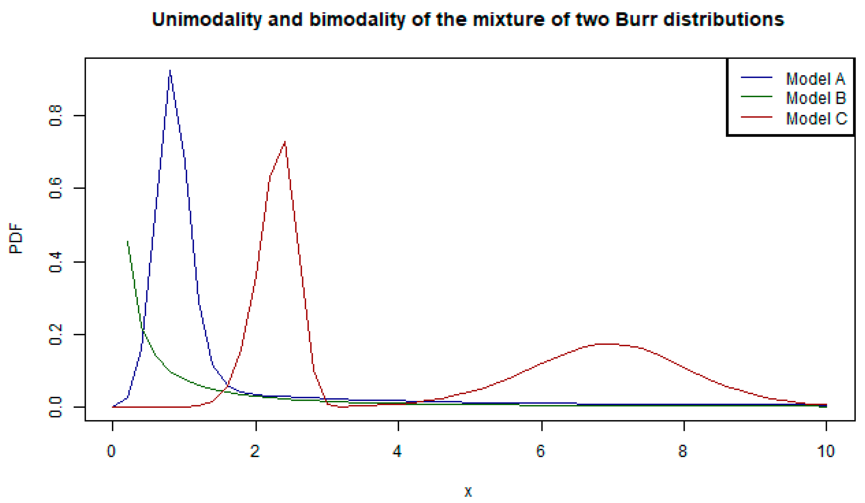
2.2.2. Flexibility for Unimodal and Multimodal Data

Abu Bakar and Nadarajah [16] illustrated the flexibility of two-component mixture models by their adaptability to unimodal and bimodal density functions. In this section, we extend the demonstration of flexibility (adaptability to unimodality and bimodality) by illustrating graphically with two additional two-component mixture models. The first model has different parametric distributions (i.e., inverse transformed gamma and transformed beta distributions) and the second has the same parametric distribution (i.e., Burr distributions) with different parameters. Varying the parameter estimates as indicated in Table 1 leads to different shapes of the pdfs in Figure 1 to illustrate how the mixture of inverse transformed gamma and transformed beta tends to account for unimodality and bimodality.
Similarly, varying the parameter estimates as indicated in Table 2 leads to different shapes of the pdfs in Figure 2 to illustrate how the mixture of two Burr distributions tends to account for unimodality and bimodality. Note that similar patterns can be illustrated for other types of mixture distributions.

2.2.3. Risk Measures

The theoretical estimate for the VaR of the mixture model does not have a closed-form solution and requires a numerical solution of
F X V a R p X = p
which can be evaluated using software as stated in [14]. However, for the mixture model, the theoretical estimate for the TVaR of X can be simplified by the “linearity” property stated in [14] to give the weighted sum of the T V a R p X of each of the component distributions.

2.3. Model Selection Criteria

This section discusses some commonly used model selection criteria that appear in the area of loss distributions. Three information criteria are considered: NLL, AIC, and BIC; see Abu Bakar et al. [7]. The BIC is also known as the Schwarz’s Bayesian Criterion (SBC). For all three criteria, a lower value implies that the theoretical model provides a better fit to the data. The NLL is appropriate only when comparing models with the same number of parameters; however, the AIC and BIC are more appropriate for comparing models with a different number of parameters. Let l θ denote the maximised log-likelihood function of a model, then the NLL is defined as
N L L = l θ .
The AIC was introduced by Akaike [24] and is defined as
A I C = 2 N L L + 2 p ,
where p is the number of free parameters or degrees of freedom. The BIC was introduced by Schwarz [25] and it is defined as
B I C = 2 N L L + p log n ,
where n is the number of observations. An analysis of the results is given with an emphasis on the BIC.

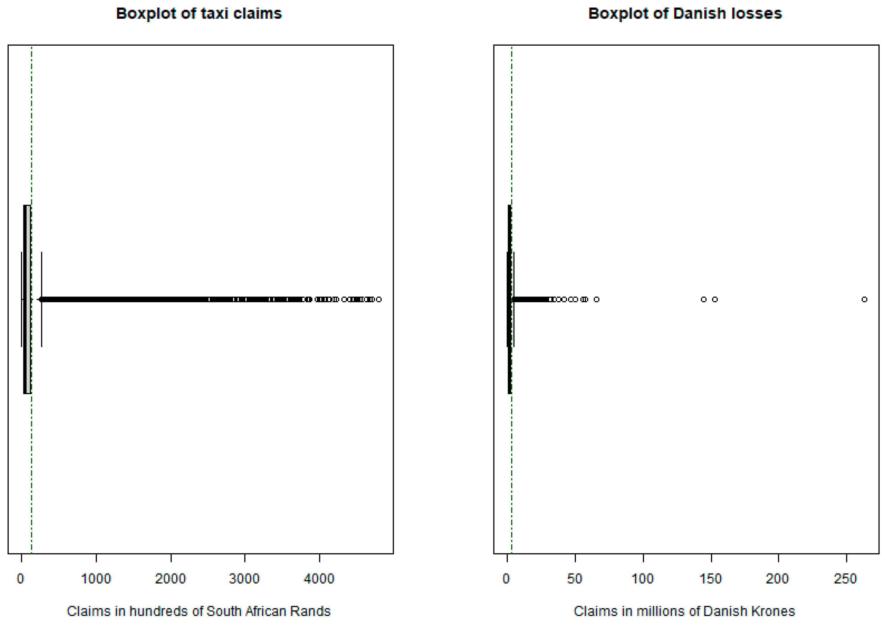
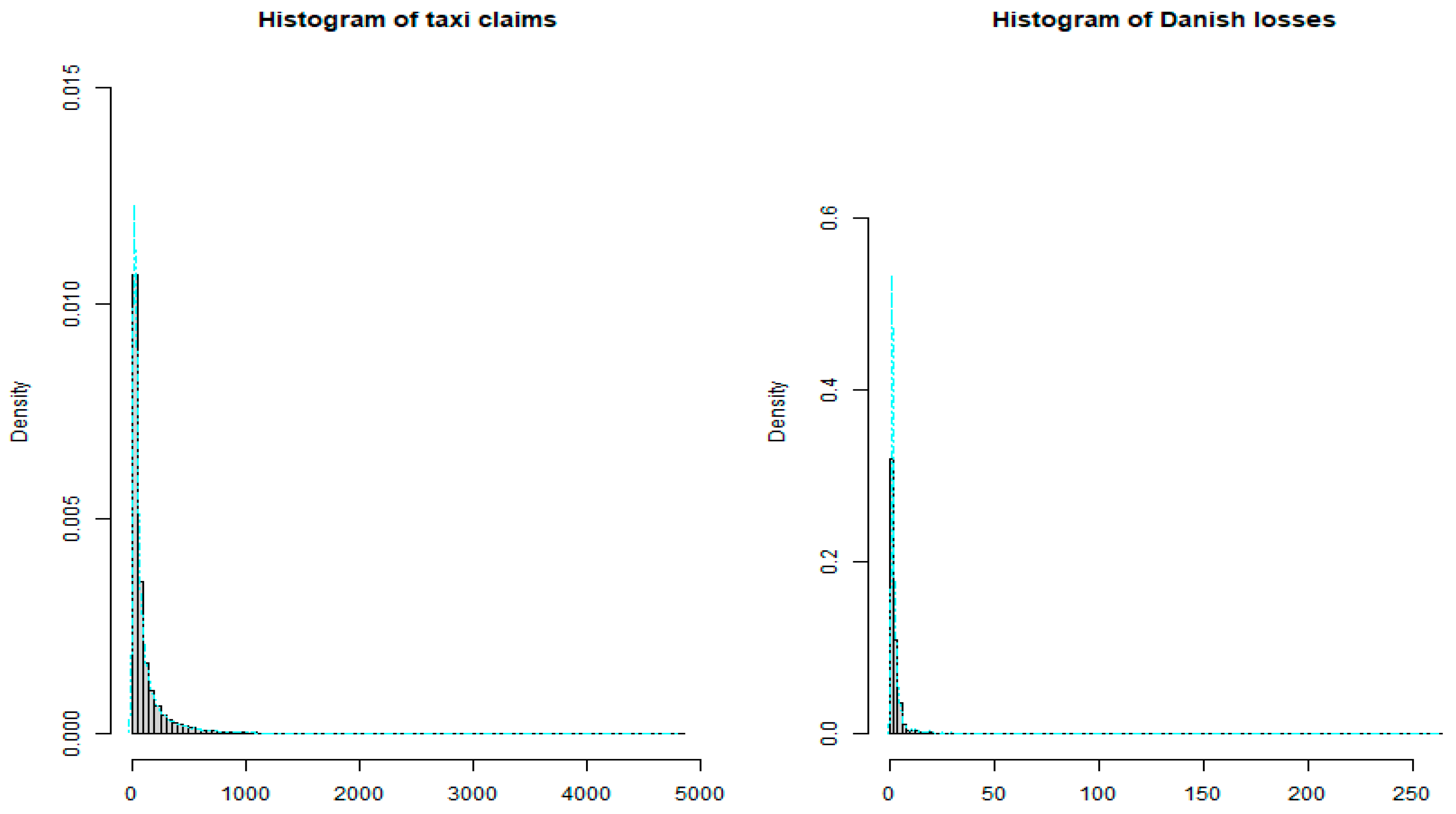
3. Empirical Analysis

In this section, the statistical computations were performed in R (R Core Team, [26]). Two real-life datasets are considered—the South African taxi claims data and the Danish fire insurance loss data. The taxi (or minibus) industry in South Africa, well known for its taxi turf wars, provides the most commonly used mode of public transport, especially for lower-income communities (which account for a larger proportion of the population due to South Africa’s high level of inequality in income levels and high unemployment rates). The types of disasters that this industry faces include and are not limited to road accidents (due to potholes, tyre bursts, improper road infrastructure, vehicle malfunctioning, and drunk driving), hijacking, theft of taxi parts, and damage or fires due to public protests because of poor service delivery by elected officials. However, the Danish fire loss data, which was collected by Copenhagen Reinsurance, covers losses from fire due to buildings, contents, and profits. The Danish data is from Denmark, which is in Europe (Northern Hemisphere), a developed first-world country, whereas the South African taxi claims data is from South Africa, which is in the southernmost part of Africa in the Southern Hemisphere, a developing third-world country. Considering that Denmark is a well-developed country, in the case of a fire hazard, the fire can be extinguished quickly because of Denmark’s well-developed social service delivery. On the other hand, with the many hazards that can occur in the taxi industry in South Africa, they may not all be avoidable because of the many underdevelopments. When it comes to economic development, a large portion of the South African population is impoverished and burdened with unemployment, whereas only a small portion of the population in Denmark is lacking.
The South African taxi claims data, which was kindly provided for our study by [23] (this data has been made available in the Supplementary Materials of this paper), consists of 48,043 observations and was divided by 100 for computational ease. The Danish fire loss data, however, is very popular and has a long history of applications. It consists of 2492 observations which were adjusted for inflation to reflect 1985 values. Most of the composite models in actuarial literature have used the Danish data as an application. The Danish dataset is available in the SMPracticals package Version 1.4-3 in R, Davidson [27]. The full R code used for the analysis in this paper has been made available in the Supplementary Materials of this paper. Table 3 and Table 4 provide the summary of the descriptive statistics for the South African taxi claims data and Danish fire loss data, respectively.
Figure 3 provides the boxplots for the South African taxi claims data and the Danish fire loss data, respectively. The dotted vertical line represents the mean value for the datasets. For both datasets, it is clear that the data are skewed to the right.
Figure 4 displays the histograms of the taxi claims and the Danish fire loss data, respectively. By visual inspection of the histograms, the claims data are positive (or at least nonnegative), unimodal and hump-shaped, skewed to the right with long upper tails, and the smaller claims occur with more frequency whereas the larger claims are less frequent.
Figure 5 displays the mean excess plots of the taxi claims on the left and the Danish fire losses data on the right. The mean excess plot for the taxi claims data is initially ultimately increasing, then ultimately constant, and then ultimately decreasing for the remainder of the plot. Therefore, the underlying distribution of the taxi claims data can be said to be heavy-tailed for the lower (left) tail and light-tailed for the upper (right) tail. The mean excess plot for the Danish losses is ultimately increasing (with two observations being the exception). Therefore, the underlying distribution of the Danish data can be said to be heavy-tailed throughout, apart from two observations.
It is important to note that the approach used in this paper is based on the ‘single best model’ as performed in well-known studies like [7,8,14,16]. That is, using the BIC (as the main model selection criteria), we extract the top 20 best goodness-of-fit models, calculate the corresponding risk metrics, and select the model with the VaR and/or TVaR closer to the corresponding empirical values. Note though that Blostein and Miljkovic [28] as well as Miljkovic and Grün [29] suggested two alternative methods to select the optimal model, which consider both the goodness-of-fit measures and the risk metrics. It is worth mentioning that [29] stated that the ‘single best model’ approach is still the most used one because although “model averaging has been recognized in the actuarial field, it has not yet been embraced as a standard practice neither in risk management nor the regulatory capital environment”, but researchers and practitioners are starting to realise the importance of applying the ‘model averaging approach’.
  • Fitting composite models to the taxi claims data
Using the 16 loss distributions outlined in Appendix A’s Table A1, it is observed in Table 5 that using distributions such as the gamma, loglogistic, paralogistic, and inverse paralogistic in the head is found to be ideal for modelling the small and moderate size claims of the taxi claims data. However, the tail distributions such as the Weibull, inverse Gaussian, Burr, Pareto, or generalised Pareto and lognormal seem to be the best choices for modelling the upper tail of taxi claims. In an effort to conserve writing space, the corresponding parameter estimates of the top 20 models in Table 5 are provided in Table A2 in Appendix A.
Table 6 reports the empirical risk estimates, the estimated risk measures for the top 20 composite models for taxi claims, and the percentage deviation in parenthesis of each estimated risk measure with respect to the empirical risk estimates. The risk estimates obtained from using the top 20 composite distributions closely match the empirical risk estimates. However, using the lognormal or the generalised Pareto distributions as a tail distribution leads to much higher estimates for the TVaR than when using the Burr distribution, the Pareto distribution, or the Weibull distribution. Using the inverse Gaussian distribution as the tail distribution leads to TVaR estimates that are much lower than the empirical estimates.
  • Fitting mixture models to the taxi claims data
Using the 16 loss distributions outlined in Appendix A’s Table A1, it is observed from the results in Table 7 that the lognormal distribution seems to be an ideal component distribution for most of the best-fitting mixture models. It seems that the conclusion by Maphalla et al. [23] that the lognormal distribution is the best for taxi claims data is supported by the top mixture models with a lognormal distribution component. In an effort to conserve writing space, the corresponding parameter estimates of the top 20 models in Table 7 are provided in Table A3 in Appendix A.
For the taxi claims data, the two-component Burr mixture also performs better than the two-component gamma mixture, the two-component Pareto mixture, the two-component Weibull mixture, and the two-component exponential mixture—this is similar to the results observed in Abu Bakar et al. [15] for the Danish, Belgian, and Norwegian loss datasets. Additionally, for the taxi claims data, the two-component paralogistic mixture performs better than the two-component Burr based on the BIC. In fact, the two-component gamma mixture, the two-component exponential mixture, and the two-component Weibull mixture did not converge for the taxi claims data. Other components such as the paralogistic distribution, the Burr distribution, the generalised Pareto distribution, the loglogistic distribution, and the inverse gamma distribution also seem to be optimal component distributions for the mixture models for the taxi claims data.
The mixture models considered provide fair estimates for the VaR at both 95% and 99% security levels, although the VaR at a 95% security level is underestimated by all the models (see Table 8). The TVaR at both 95% and 99% security levels is not underestimated for any of the models, which provides a bit of comfort since the TvaR is a coherent risk measure and more attractive than the VaR.
  • Fitting composite models to the Danish data
Using the 16 loss distributions outlined in Appendix A’s Table A1, it is observed that having distributions such as the Weibull, paralogistic, and inverse Burr in the head is found to be ideal for modelling the small and moderate size claims of Danish fire losses (Grün and Miljkovic, [8]). The tail distributions such as inverse Weibull, inverse paralogistic, loglogistic, Burr, inverse gamma, and paralogistic seem to be the best choices for modelling the long tail of Danish fire losses (Grün and Miljkovic, [8]). In an effort to conserve writing space, the corresponding parameter estimates of the top 20 models in Table 9 are provided in Table A4 in Appendix A.
Although the composite inverse Burr-Burr model has the lowest NLL and AIC among the other models in Table 9 (and the 256 considered), there is no strong evidence that it provides a better fit than the other models—its BIC is not at least 10 units less than the BIC of the other models in Table 9 (see Abu Bakar et al. [7]). Additionally, the composite inverse Burr-Burr model has six parameters, and the principle of parsimony does not favour it. Rather, a simpler four-parameter composite model is more favourable here.
Table 10 reports the empirical risk estimates, the estimated risk measures for the top 20 composite models for Danish fire loss data and the percentage deviation in parenthesis of each estimated risk measure with respect to the empirical risk estimates. Most of the risk estimates in Table 10 obtained from using the top 20 composite distributions closely match the empirical risk estimates (except those with the Burr as the tail distribution, in terms of the TVaR). The top 20 composite models provide fair estimates for the VaR at both 95% and 99% security levels, although the VaR at a 95% security level is underestimated by all the models (see Table 10). Using the Burr distribution as a tail distribution leads to much higher estimates for the TVaR than using the inverse Weibull distribution, the inverse paralogistic distribution, or the loglogistic distribution. Using the inverse gamma or the paralogistic distribution as the tail distribution leads to TVaR estimates that are lower than the empirical estimates at a 95% security level.
  • Fitting mixture models to the Danish data
Using the 16 loss distributions outlined in Appendix A’s Table A1, it is observed from the results in Table 11 that the Burr distribution seems to be an ideal component distribution for most of the best mixture models. For the Danish fire loss data, the two-component Burr mixture performs better than the two-component gamma mixture, the two-component Pareto mixture, the two-component Weibull mixture, and the two-component exponential mixture as also concluded in Abu Bakar et al. [15] for the three fire loss datasets considered (i.e., Danish, Belgian and Norwegian). In an effort to conserve writing space, the corresponding parameter estimates of the top 20 models in Table 11 are provided in Table A5 in Appendix A.
Other than the Burr distribution, the inverse Weibull distribution and the inverse gamma distribution also seem like optimal component distributions for the mixture models of the Danish fire loss data.
Table 12 reports the empirical risk estimates, the estimated risk measures for the top 20 mixture models for the Danish fire loss data, and the percentage deviation in parenthesis of each estimated risk measure with respect to the empirical risk estimates. The mixture distributions considered provide fair estimates for the VaR at both 95% and 99% security levels. Most of the mixture models have TVaR estimates much higher than the empirical estimates. For the Danish data, the mixture models proposed, especially the ones with the Burr component, do not adequately capture the area under the tail.
Finally, although the results in Table 5, Table 7, Table 9 and Table 11 are sorted in terms of the BIC (in the last column), the boldfaced value in each column provides the best goodness of fit with respect to the minimum model selection criterion (NLL, AIC, BIC).

4. Conclusions

For the composite models, it seems that the composite Paralogistic-Burr, composite Weibull-Burr, and composite Inverse Burr-Burr are optimal models for both datasets as they both appear in the top 20 composite models. However, for the mixture models, it seems that the two-component Burr mixture, the two-component paralogistic and Burr mixture, and the two-component lognormal and Burr mixture are optimal models for both datasets as they also both appear in the top 20 mixture models. In general, the composite models provide better risk estimates for both of the datasets. The mixture models seem to not adequately capture the area under the tail, especially when using the Burr distribution as a component distribution for the Danish data. Finally, model selection criteria (NLL, AIC, BIC) evaluate the quality of fit of the entire model and not just the tail, so both the model selection criteria and risk estimates are important for deciding which model is optimal.
As it can be observed here, there is no single universal composite or mixture model that is better than the others. Stated differently, the best model depends on the underlying data being used to fit the model and the corresponding risk metrics. Finally, care needs to be taken when interpreting the risk metrics because a model with an excessively large risk metric as compared to the empirical estimate implies that more funds need to be kept in reserve rather than being invested elsewhere, which leads to less profits.
For future research, composite and mixture models (with more than two components) can be fitted to the taxi claims data to evaluate their suitability and other appropriate risk metrics. More importantly, it would be of interest to investigate what would be the best possible back-testing technique that is appropriate for the considered models and risk metrics. While a lot of composite and mixture distributions were considered in this paper, a reader can extend this list by considering the distributions that are discussed in [30]. Next, if data are time-dependent, readers are advised to also investigate analytical methods that involve hidden Markov models. Given that this paper used the ‘single best model’ approach, it would be interesting to investigate the ‘grid map’ and ‘model averaging’ methods discussed in [28,29,31,32] using the datasets and models discussed in this paper. There is also a need for academics to engage with the private sector so that they can be granted access to large datasets and be able to use more advanced and accurate machine learning techniques where data can be split into training, validation, and test sets, as well as for back-testing purposes. However, considering that the data from private companies are usually under many proprietary laws, this is a major limitation when it comes to the analysis of real-life insurance data.

Supplementary Materials

The following supporting information can be downloaded at: https://www.mdpi.com/article/10.3390/math12020335/s1. Supplementary File: R Code for Mathematics. Table S1. Taxi Claims Data.

Author Contributions

Methodology, W.A.M.; Software, W.A.M.; Validation, W.A.M. and S.C.S.; Formal analysis, W.A.M. and S.C.S.; Investigation, W.A.M. and S.C.S.; Resources, S.C.S.; Data curation, W.A.M. and S.C.S.; Writing—original draft, W.A.M.; Writing—review & editing, S.C.S. All authors have read and agreed to the published version of the manuscript.

Funding

This research received no external funding. The authors would like to acknowledge the Department of Mathematical Statistics and Actuarial Science, and the Open Access Publication Fund at University of the Free State for assistance with APC.

Data Availability Statement

The data and R codes used in this paper are provided as Supplementary Materials.

Conflicts of Interest

The authors declare no conflict of interest.

Appendix A

Table A1. Sixteen distributions that are considered as head and/or tail in the composite model, or first and second components in the mixture model.
DistributionParametersPDFCDF E X k
Burr α > 0 ,   γ > 0 ,
θ > 0
α γ x θ γ x [ 1 + x θ γ ] α + 1 1 u α ,      u = 1 1 + x θ γ θ k Γ 1 + k γ Γ α k γ Γ ( α ) , γ < k < α γ
Exponential θ > 0 e x θ θ 1 e x θ θ k Γ k + 1 ,              k > 1                            θ k k ! ,                     i f   k   i s   a   p o s i t i v e   i n t e g e r     
Gamma α > 0 ,   θ > 0 x θ α e x θ x Γ ( α ) Γ α ; x θ { θ k Γ α + k Γ α ,                      k > α   θ k α + k 1 α ,       i f   k   i s   a   p o s i t i v e   i n t e g e r            
Generalised Pareto α > 0 ,   τ > 0 ,
θ > 0
Γ α + τ Γ α Γ τ θ α x τ 1 ( x + θ ) α + τ β τ , α ; u ,      u = x x + θ θ k Γ τ + k Γ α k Γ α Γ τ ,            τ < k < α                θ k τ ( τ + 1 ) ( τ + k 1 ) ( α 1 ) ( α k ) ,   i f   k   i s   a   p o s i t i v e   i n t e g e r  
Inverse Burr τ > 0 ,   γ > 0 ,  
θ > 0
τ γ x θ γ τ x [ 1 + x θ γ ] τ + 1 u τ ,      u = x θ γ 1 + x θ γ θ k Γ ( τ + k γ ) Γ ( 1 k γ ) Γ ( τ ) , τ γ < k < γ
Inverse Exponential θ > 0 θ e θ x x 2 e θ x θ k Γ 1 k ,    k < 1
Inverse Gamma α > 0 ,   θ > 0 θ x α e θ x x Γ ( α ) 1 Γ α ; θ x θ k Γ α k Γ α   ,             i f   k < α                θ k ( α 1 ) ( α k ) ,   i f   k   i s   a   p o s i t i v e   i n t e g e r           
Inverse Gaussian μ > 0 ,   θ > 0 θ 2 π x 3 1 2 e θ z 2 2 x ,
z = x μ μ
Φ z θ x 1 2 + e 2 θ μ Φ y θ x 1 2
z = x μ μ
n = 0 k 1 k + n 1 ! k n 1 ! n ! μ n + k 2 θ n ,    k = 1 , 2 , ,
Inverse Paralogistic τ > 0 ,   θ > 0 τ 2 x θ τ 2 x 1 + x θ τ τ + 1 u τ ,      u = x θ τ 1 + x θ τ θ k Γ τ + k τ Γ 1 k τ Γ τ , τ 2 < k < τ
Inverse Pareto τ > 0 ,   θ > 0 τ θ x τ 1 ( x + θ ) τ + 1 x x + θ τ θ k Γ τ + k Γ 1 k Γ τ , τ < k < 1     θ k ( k ) ! ( τ 1 ) ( τ + k ) , i f   k   i s   a   n e g a t i v e   i n t e g e r    
Inverse Weibull τ > 0 ,   θ > 0 τ θ x τ e θ x τ x e θ x τ θ k Γ 1 k τ ,   k < τ
Loglogistic γ > 0 ,   θ > 0 γ x θ γ x [ 1 + x θ γ ] 2 x θ γ 1 + x θ γ θ k Γ 1 + k γ Γ 1 k γ , γ < k < γ
Lognormal μ > 0 ,   σ > 0 1 x σ 2 π e z 2 2 = ϕ z σ x
z = l n x μ σ
Φ z e k μ + 1 2 k 2 σ 2
Paralogistic α > 0 ,   θ > 0 α 2 x θ α x [ 1 + x θ α ] α + 1 1 u α ,      u = 1 1 + x θ α θ k Γ ( 1 + k α ) Γ ( α k α ) Γ ( α ) , α < k < α 2
Pareto α > 0 ,   θ > 0 α θ α ( x + θ ) α + 1 1 θ x + θ α θ k Γ k + 1 Γ α k Γ α ,                    1 < k < α      θ k k ! ( α 1 ) ( α k ) ,    i f   k   i s   a   p o s i t i v e   i n t e g e r   
Weibull τ > 0 ,   θ > 0 τ x θ τ e x θ τ x 1 e x θ τ θ k Γ 1 + k τ ,   k > τ
Table A2. Parameter estimates and standard errors in parenthesis of the top 20 composite models for the taxi claims data.
HeadTail ϑ 1 ϑ 2 θ ϕ
GammaWeibull α = 1.8955   ( 0.0229 ) ,
1 θ = 0.0599 ( 0.0014 )
τ = 0.3325   ( 0.0058 ) ,
θ = 7.1857 ( 0.72095 )
35.5261 1.3957
ParalogisticInverse Gaussian α = 1.6984 ( 101.315 ) ,
1 θ = 0.0231 ( 17.4617 )
μ = 101.31497   ( 3.7430 ) ,
θ = 17.46168   ( 1.4671 )
37.1193 1.2982
LoglogisticInverse Gaussian γ = 1.7352   ( 0.0155 ) ,
θ = 32.5366   ( 0.4623 )
μ = 99.64726   ( 4.2422 ) ,
θ = 16.8705   ( 1.6193 )
40.5153 1.1594
ParalogisticWeibull α = 1.7090   ( 0.0154 ) ,
1 θ = 0.02368   ( 0.0003 )
τ = 0.3338   ( 0.0058 ) ,
θ = 7.3820   ( 0.735 )
34.7893 1.4319
Inverse paralogisticInverse Gaussian τ = 1.3895   ( 0.0072 ) ,
1 θ = 0.0364   ( 0.0005 )
μ = 91.2859   ( 6.0897 ) ,
θ = 14.0619   ( 2.0543 )
51.2797 0.8695
WeibullWeibull τ = 1.6529   ( 0.0166 ) ,
θ = 28.8585   ( 0.4634 )
τ = 0.3376205   ( 0.0058 ) ,
θ = 7.9324   ( 0.76697 )
30.8894 1.6791
GammaBurr α = 1.8953 ( 0.0236 ) ,
1 θ = 0.05999   ( 0.0015 )
α = 9290451 ( 2166981 ) ,
γ = 0.3324   ( 0.0061 ) ,
1 θ = 1.519089 × 10 22   ( 1.195389 × 10 23 )
35.5336 1.3953
LoglogisticWeibull γ = 1.7465   0.016 ,
θ = 31.722669
τ = 0.3335 0.0058 ,
θ = 7.3185 0.7314
37.162 1.314
ParalogisticBurr α = 1.7090   0.0152   ,
θ = 0.0237 0.0003
α = 132231.5 , γ = 0.3338 ,
1 θ = 6.186885 × 10 17
34.7898 1.4319
WeibullBurr τ = 1.6528   ( 0.0166 ) ,
θ = 28.8594   0.4602
α = 873910.9 ,
γ = 0.3376 0.0057 ,
1 θ = 3.173873 × 10 19
30.891 1.6789
Inverse BurrWeibull τ = 0.8631   0.0595 ,
γ = 1.9451   0.1031 ,
1 θ = 0.0301 0.0007
τ = 0.3341   0.0058 ,
θ = 7.4239 0.7363
35.0194 1.4186
LoglogisticBurr γ = 1.7465   ( 0.0156 ) ,
θ = 31.7227   ( 0.41667 )
α = 31127.62 , γ = 0.3335 ,
1 θ = 4.603593 × 10 15
37.1616 1.3140
Inverse BurrBurr τ = 0.8632 0.0599     ,
γ = 1.9450   0.1035   ,
1 θ = 0.03012 0.00066
α = 18358.92   , γ = 0.334237 ,
1 θ = 2.354395 × 10 14
35.01608 1.4188
Inverse paralogisticWeibull τ = 1.3941 ( 0.0077 ) ,
1 θ = 0.0372   ( 0.0006 )
τ = 0.3313   0.0062 ,
θ = 6.9658   0.7622
44.1095 1.0634
Inverse paralogisticBurr τ = 1.3941 ( 0.0077 ) ,
1 θ = 0.0372   ( 0.0006 )
α = 29397.29 ,
γ = 0.3313 ( 0.0006 ) ,
1 θ = 4.6688 × 10 15   ( 1.0827 × 10 17 )
44.1084 1.0634
BurrPareto α = 0.3761   ( 0.0112 ) ,
γ = 1.8324   ( 0.0187 ) ,
1 θ = 0.0487   ( 0.0010 )
α = 2.6827   ( 0.164 ) ,
θ = 443.996   ( 61.2433 )
371.0913 0.0883
WeibullLognormal τ = 1.68   ( 0.0180 ) ,
θ = 27.3341   ( 0.5253 )
μ = 3.2995   ( 0.0398 ) ,
σ = 1.6521   ( 0.0180 )
27.3694 2.0122
GammaLognormal α = 1.9054   ( 0.0247 ) ,
1 θ = 0.0614   ( 0.0017 )
μ = 3.2496   ( 0.0443 ) ,
σ = 1.6686   ( 0.0188 )
32.3335 1.6029
GammaGeneralised Pareto α = 1.9193   ( 0.0243 ) ,
1 θ = 0.063   ( 0.0016 )
α = 2.00855   ( 0.0590 ) ,
τ = 0.00000008   ( 1.4945 × 10 15 ) ,
1 θ = 0.00263   ( 0.00015 )
33.0272 1.5616
ParalogisticLognormal α = 1.7207 ( 0.0264 ) ,
1 θ = 0.0243 ( 0.0005 )
μ = 3.2653 ( 0.0550 ) ,
σ = 1.6637   ( 0.0264 )
30.9552 1.6977
Table A3. Parameter estimates of the top 20 mixture models for the taxi claims data.
First ComponentSecond Component ϑ 1 ϑ 2 ϕ
Inverse gammaLognormal α = 3.8170 ,   θ = 93.6396 μ = 4.074 ,   σ = 1.4041 4.4276
Inverse GaussianLognormal μ = 29.8338 ,   θ = 107.9798 μ = 4.0794 ,   σ = 1.3961 4.7267
Generalised ParetoLognormal α = 4.1712 ,   τ = 45.299 ,
θ = 2.2854
μ = 4.0765 ,   σ = 1.4031 4.4435
Inverse paralogisticLognormal τ = 2.4166 ,   θ = 17.1673 μ = 4.0813 ,   σ = 1.4069 4.0799
Inverse WeibullLognormal τ = 2.0034 θ = 23.086563 μ = 4.060686 ,   σ = 1.4098 4.1863
Inverse BurrLognormal τ = 4.5381 ,   γ = 2.1940 ,
θ = 12.0926
μ = 4.0736 ,   σ = 1.4101 4.0411
LoglogisticLognormal γ = 2.9332 ,   θ = 26.4047 μ = 4.1085 ,   σ = 1.3974 3.9066
BurrLognormal α = 0.5817 ,   γ = 3.4263 ,
θ = 21.4809
μ = 4.0956802 , σ = 1.4086 3.6253
GammaLognormal α = 4.2428 ,   θ = 6.5837 μ = 4.091793 ,   σ = 1.3857 4.769
ParalogisticLognormal α = 2.403 ,   θ = 40.2599 μ = 4.126997 ,   σ = 1.3822 4.002
LognormalWeibull μ = 4.1531 ,   σ = 1.3612 τ = 1.9636 ,   θ = 29.5290 0.2536
LoglogisticGeneralised Pareto γ = 1.7759 ,   θ = 29.8996 α = 2.2800 ,    τ = 1.5141 ,
θ = 247.543
0.52375
Generalised ParetoParalogistic α = 2.0570 ,   τ = 1.614 ,
θ = 168.3791
α = 1.7326 ,   θ = 39.1302 1.1726
LoglogisticParalogistic γ = 1.7641 ,   θ = 30.5826 α = 1.3814 ,   θ = 228.3339 0.4576
BurrLoglogistic α = 1.6342 ,   γ = 1.2558 ,
θ = 256.4782
γ = 1.7836 ,   θ = 30.326 1.9518
ParalogisticParalogistic α = 1.7332 ,   θ = 40.1747 α = 1.3464 ,    θ = 180.1915 0.7779
BurrBurr α = 0.95765 ,   γ = 1.7884 ,
θ = 29.6828
α = 1.663 ,   γ = 1.2498 ,
θ = 264.2923
0.4903
Inverse gammaParalogistic α = 1.7495 ,   θ = 294.6358 α = 1.6836 ,   θ = 43.7961 2.4313
Inverse gammaGeneralised Pareto α = 1.8386 ,    θ = 334.996 α = 6.2739 ,   τ = 1.9704 ,
θ = 107.74715
2.2563
ParalogisticBurr α = 1.7378 ,   θ = 40.1805 α = 1.3951 ,   τ = 1.3194 ,
θ = 184.542
0.797
Table A4. Parameter estimates and standard errors in parenthesis of the top 20 composite models for the Danish fire loss data.
HeadTail ϑ 1 ϑ 2 θ ϕ
WeibullInverse Weibull τ = 16.094 ( 1.554 ) ,
θ = 0.955 ( 0.0149 )
τ = 1.555 ( 0.0505 ) ,
1 θ = 1.102 ( 0.0994 )
0.955 9.854
ParalogisticInverse Weibull α = 16.088 ( 1.581 ),
1 θ = 0.879 ( 0.0232 )
τ = 1.554 ( 0.0507 ) ,
1 θ = 1.105 ( 0.101 )
0.957 9.688
Inverse BurrInverse Weibull τ = 0.204 ( 0.235 ) ,
γ = 68.745 ( 73.872 ,
1 θ = 1.046 ( 0.0176 )
τ = 1.557 ( 0.0493 ) ,
1 θ = 1.096 ( 0.0919 )
0.934   12.609
WeibullInverse paralogistic τ = 15.806 ( 1.728 ) ,
θ = 0.960 ( 0.0176 )
τ = 1.567 ( 0.0565 ) ,
1 θ = 1.777 ( 0.213 )
0.961   9.256
Inverse BurrInverse paralogistic τ = 0.000383 ( 0.00001 ) ,
γ = 35290 ( 1049 ) ,
1 θ = 1.078 ( 0.00005 )
τ = 1.567 ( 0.053 ) ,
1 θ = 1.775 ( 0.181 )
0.928 14.086
ParalogisticInverse paralogistic α = 15.745 ( 1.968 ) ,
1 θ = 0.872 ( 0.0301 )
τ = 1.566 0.057 ,
1 θ = 1.787 0.221
0.964 9.054
WeibullLoglogistic τ = 15.652 ( 1.939 ) ,
θ = 0.962 ( 0.0206 )
γ = 1.568 ( 0.0593 ) ,
θ = 0.680 ( 0.0979 )
0.964 9.030
Inverse BurrLoglogistic τ = 0.000395 ( 0.00002 ) ,
γ = 34285 ( 1.517 ) ,
1 θ = 1.078 ( 0.00005 )
γ = 1.570 ( 0.0278 ) ,
θ = 0.688 ( 0.00275 )
0.928 14.020
ParalogisticLoglogistic α = 15.683 ( 1.205 ) ,
1 θ = 0.871 ( 0.0174 )
γ = 1.567 ( 0.0569 ) ,
θ = 0.678 ( 0.0888 )
0.965 8.906
LoglogisticInverse Weibull γ = 16.267 ( 1.264 ) ,
θ = 0.975 ( 0.0127 )
α = 1.547 ( 0.0502 ) ,
1 θ = 1.130 ( 0.105 )
0.976 8.216
WeibullBurr τ = 16.267 ( 1.264 ) ,
θ = 0.949 ( 0.00107 )
α = 0.395 0.104 ,
γ = 3.646 0.880 ,
1 θ = 1.182 ( 0.0693 )
0.947 11.13
ParalogisticBurr α = 16.278 ( 1.257 ) ,
1 θ = 0.887 ( 0.887 )
α = 0.394 ( 0.104 ) ,
γ = 3.649 ( 0.884 ) ,
1 θ = 1.182 ( 0.0697 )
0.947 11.043
Inverse BurrBurr τ = 0.262 ( 0.108 ) ,
γ = 53.766 ( 19.976 ) ,
1 θ = 1.046 ( 0.0099 )
α = 0.406 ( 0.107 ) ,
γ = 3.549 ( 0.853 ) ,
1 θ = 1.190 ( 0.0713 )
0.932 13.251
LoglogisticInverse paralogistic γ = 16.197 ( 1.358 ) ,
θ = 0.977 ( 0.0141 )
τ = 1.561 0.0554 ,
1 θ = 1.819 ( 0.216 )
0.980 7.876
Inverse BurrInverse gamma τ = 4.4300 ( 0.000000225 ) ,
γ = 30761 ( 0.885 ) ,
1 θ = 1.078 ( 0.0000315 )
α = 1.641 ( 0.0399 ) ,
1 θ = 1.148 ( 0.0263 )
0.928 13.945
ParalogisticInverse gamma α = 15.635 ( 1.285 ) ,
1 θ = 0.869 ( 0.0186 )
α = 1.635 ( 0.0733 ) ,
1 θ = 1.119 ( 0.188 )
0.967 8.753
LoglogisticLoglogistic γ = 16.153 ( 1.387 ) ,
θ = 0.978 ( 0.0145 )
γ = 1.562 ( 0.0573 ) ,
θ = 0.666 ( 0.0911 )
0.981 7.761
WeibullParalogistic τ = 15.511 ( 1.314 ) ,
θ = 0.965 ( 0.00129 )
α = 1.267 ( 0.0273 ) ,
1 θ = 1.607 ( 0.265 )
0.968 8.660
ParalogisticParalogistic α = 15.557 ( 1.3555 ) ,
1 θ = 0.867 ( 0.020 )
α = 1.266 ( 0.0273 ) ,
1 θ = 1.611 ( 0.267 )
0.969 8.551
Inverse BurrParalogistic τ = 0.000929 ( 0.0000014 ) ,
γ = 14718 ( 2.036 ) ,
1 θ = 1.077 ( 0.0000152 )
α = 1.270 ( 0.0136 ) ,
1 θ = 1.559 ( 0.0307 )
0.928 13.775
Table A5. Parameter estimates of the top 20 mixture models for the Danish fire loss data.
First ComponentSecond Component ϑ 1 ϑ 2 ϕ
BurrBurr α = 0.2706 ,   γ = 6.6542 ,
θ = 1.2869
α = 0.0257 ,   γ = 49.3079 ,   θ = 0.8573 2.1565
Inverse WeibullBurr τ = 10.5701 ,   θ = 0.9465 α = 0.1577 ,   γ = 9.0711 ,   θ = 1.1658 4.3468
LoglogisticBurr γ = 5.1028 ,   θ = 1.7185 α = 0.028 ,   γ = 41.8835 ,   θ = 0.8645 4.6562
Inverse paralogisticBurr γ = 11.85025 ,   θ = 0.7666 α = 0.1541 ,   γ = 9.2683 ,   θ = 1.1497 4.7785
Inverse BurrBurr τ = 136.2773 ,   γ = 10.6678 ,
θ = 0.5971
α = 0.1574 ,    γ = 9.0858 ,   θ = 1.1646 4.3782
GammaBurr α = 8.7777 ,   θ = 0.2029 α = 0.0298 ,   γ = 39.7623 ,   θ = 0.8677 5.40768
Inverse GaussianBurr μ = 2.1500 ,   θ = 8.79 α = 0.0315 ,   γ = 38.8700 ,   θ = 0.8699 4.7799
LognormalBurr μ = 0.6349 ,   σ = 0.4417 α = 0.0308 ,   γ = 39.48825 ,   θ = 0.8686 4.7594
Generalised ParetoBurr α = 12.2499 ,   τ = 10.915 ,
θ = 2.0900
α = 0.0303 ,   γ = 39.960 ,   θ = 0.8679 4.7499
Inverse gammaBurr α = 3.6500 ,   θ = 6.61997 α = 0.0404 ,   γ = 31.330 ,   θ = 0.877 4.2999
Inverse exponentialBurr θ = 0.98115 α = 0.04097 ,    γ = 25.728 ,   θ = 0.8903 134.9374
ExponentialBurr 1 θ = 0.3686 α = 0.04999 ,    γ = 25.2807 ,    θ = 0.8908 119.5614
Inverse ParetoBurr τ = 66.423 ,   θ = 0.015575 α = 0.0491 , γ = 25.7105 ,   θ = 0.8903 134.9823
ParalogisticBurr α = 20.0916 ,   θ = 1.1077 α = 0.1294 , γ = 10.7409 ,   θ = 1.0445 10.19554
WeibullBurr τ = 19.9054 ,   θ = 0.95505 α = 0.1291 ,   γ = 10.7569 ,    θ = 1.0427 10.3812
ParetoBurr α = 37.699 ,   θ = 100.9595 α = 0.0501 ,   γ = 25.2500 ,   θ = 0.8908 121.669
Inverse WeibullInverse Burr τ = 3.9523 ,   θ = 1.1564 τ = 5.8476 ,   γ = 1.714638 ,   θ = 0.866 0.7465
Inverse paralogistic Inverse Weibull τ = 1.9012 ,   θ = 2.3835 τ = 3.4688 ,   θ = 1.2099 2.2879
Inverse gammaInverse Weibull α = 3.6924 ,   θ = 1.183 τ = 1.91129 ,   θ = 4.8491 0.6334
Inverse BurrInverse Burr τ = 5.8468 ,   γ = 1.7148 ,    θ = 0.866 τ = 4119.4997 ,    γ = 3.9533 ,   θ = 0.1408 1.33905

References

  1. Cooray, K.; Ananda, M.M.A. Modeling actuarial data with a composite lognormal-Pareto model. Scand. Actuar. J. 2007, 2005, 321–334. [Google Scholar] [CrossRef]
  2. Scollnik, D.P.M. On composite lognormal-Pareto models. Scand. Actuar. J. 2007, 2007, 20–33. [Google Scholar] [CrossRef]
  3. Pigeon, M.; Denuit, M. Composite Lognormal-Pareto model with random threshold. Scand. Actuar. J. 2010, 2011, 177–192. [Google Scholar] [CrossRef]
  4. Nadarajah, S.; Bakar, S.A.A. New composite models for the Danish fire insurance data. Scand. Actuar. J. 2012, 2014, 180–187. [Google Scholar] [CrossRef]
  5. Ciumara, R. An actuarial model based on the composite Weibull-Pareto distribution. Math. Rep. 2006, 8, 401–414. [Google Scholar]
  6. Scollnik, D.P.M.; Sun, C. Modeling with Weibull-Pareto models. N. Am. Actuar. J. 2012, 16, 260–272. [Google Scholar] [CrossRef]
  7. Abu Bakar, S.A.; Hamzah, N.A.; Maghsoudi, M.; Nadarajah, S. Modeling loss data using composite models. Insur. Math. Econ. 2015, 61, 146–154. [Google Scholar] [CrossRef]
  8. Grün, B.; Miljkovic, T. Extending composite loss models using a general framework of advanced computational tools. Scand. Actuar. J. 2019, 2019, 642–660. [Google Scholar] [CrossRef]
  9. Calderin-Ojeda, E.; Kwok, C.F. Modeling claims data with composite Stoppa models. Scand. Actuar. J. 2015, 2016, 817–836. [Google Scholar] [CrossRef]
  10. Keatinge, C.L. Modeling losses with the mixed exponential distribution. Proc. Casualty Actuar. Soc. 1999, LXXXVI, 654–698. [Google Scholar]
  11. Klugman, S.; Rioux, J. Toward a Unified Approach to Fitting Loss Models. N. Am. Actuar. J. 2006, 10, 63–83. [Google Scholar] [CrossRef]
  12. Lee, S.C.K.; Lin, S.X. Modeling and Evaluating Insurance Losses Via mixtures of Erlang Distributions. N. Am. Actuar. J. 2010, 14, 107–130. [Google Scholar] [CrossRef]
  13. Tijms, H. Stochastic Models: An Algorithm Approach; Wiley: Hoboken, NJ, USA, 1994; ISBN 0-471-95123-4. [Google Scholar]
  14. Miljkovic, T.; Grün, B. Modeling loss data using mixtures of distributions. Insur. Math. Econ. 2016, 70, 387–396. [Google Scholar] [CrossRef]
  15. Abu Bakar, S.A.; Nadarajah, S.; Adzhar, Z.A.A.K. Loss modeling using Burr mixtures. Empir. Econ. 2017, 54, 1503–1516. [Google Scholar] [CrossRef]
  16. Abu Bakar, S.A.; Nadarajah, S. Risk measure estimation under two component mixture models with trimmed data. J. Appl. Stat. 2019, 46, 835–852. [Google Scholar] [CrossRef]
  17. Asgharzadeh, A.; Nadarajah, S.; Sharafi, F. Generalized inverse Lindley distribution with application to Danish fire insurance data. Commun. Stat. Theory Methods 2017, 46, 5000–5021. [Google Scholar] [CrossRef]
  18. Punzo, A.; Bagnato, L.; Maruotti, A. Compound unimodal distributions for insurance losses. Insur. Math. Econ. 2018, 81, 95–107. [Google Scholar] [CrossRef]
  19. Bhati, D.; Ravi, S. On generalized log-Moyal distribution: A new heavy tailed size distribution. Insur. Math. Econ. 2018, 79, 247–259. [Google Scholar] [CrossRef]
  20. Li, Z.; Beirlant, J.; Meng, S. Generalizing the log-Moyal distribution and regression models for heavy-tailed loss data. ASTIN Bull. J. IAA 2021, 51, 57–99. [Google Scholar] [CrossRef]
  21. Zhao, J.; Ahmad, Z.; Mahmoudi, E.; Hafez, E.H.; Mohie El-Din, M.M. A new class of heavy-tailed distributions: Modeling and simulating actuarial measures. Complexity 2021, 2021, 5580228. [Google Scholar] [CrossRef]
  22. Ahmad, Z.; Mahmoudi, E.; Dey, S. A new family of heavy tailed distributions with an application to the heavy tailed insurance loss data. Commun. Stat.-Simul. Comput. 2022, 51, 4372–4395. [Google Scholar] [CrossRef]
  23. Maphalla, R.; Mokhoabane, M.; Ndou, M.; Shongwe, S.C. Quantifying risk using loss distributions. In Applied Probability Theory—New Perspectives, Recent Advances and Trends; Jaoude, A.A., Ed.; IntechOpen: London, UK, 2023; pp. 139–161. [Google Scholar] [CrossRef]
  24. Akaike, H. A new look at the statistical model identification. IEEE Trans. Autom. Control 1974, 19, 716–723. [Google Scholar] [CrossRef]
  25. Schwarz, G. Estimating the Dimension of a Model. Ann. Stat. 1978, 6, 461–464. [Google Scholar] [CrossRef]
  26. R Core Team. R: A Language and Environment for Statistical Computing. 2022. Available online: https://www.R-project.org/ (accessed on 1 April 2023).
  27. Davison, A. SMPracticals: Practicals for Use with Davison (2003) Statistical Models. 2019. R Package Version 1.4-3. Available online: https://CRAN.R-project.org/package=SMPracticals (accessed on 1 May 2023).
  28. Blostein, M.; Miljkovic, T. On modeling left-truncated loss data using mixtures of distributions. Insur. Math. Econ. 2019, 85, 35–46. [Google Scholar] [CrossRef]
  29. Miljkovic, T.; Grün, B. Using Model Averaging to Determine Suitable Risk Measure Estimates. N. Am. Actuar. J. 2021, 25, 562–579. [Google Scholar] [CrossRef]
  30. Rigby, R.A.; Stasinopoulos, M.D.; Heller, G.Z.; De Bastiani, F. Distributions for Modeling Location, Scale, and Shape: Using GAMLSS in R; CRC Press: Boca Raton, FL, USA, 2019. [Google Scholar] [CrossRef]
  31. Zou, J.; Wang, W.; Zhang, X.; Zou, G. Optimal model averaging for divergent-dimensional Poisson regressions. Econom. Rev. 2022, 41, 775–805. [Google Scholar] [CrossRef]
  32. Zou, J.; Yuan, C.; Zhang, X.; Zou, G.; Wan, A.T.K. Model averaging for support vector classifier by cross-validation. Stat. Comput. 2023, 33, 117. [Google Scholar] [CrossRef]
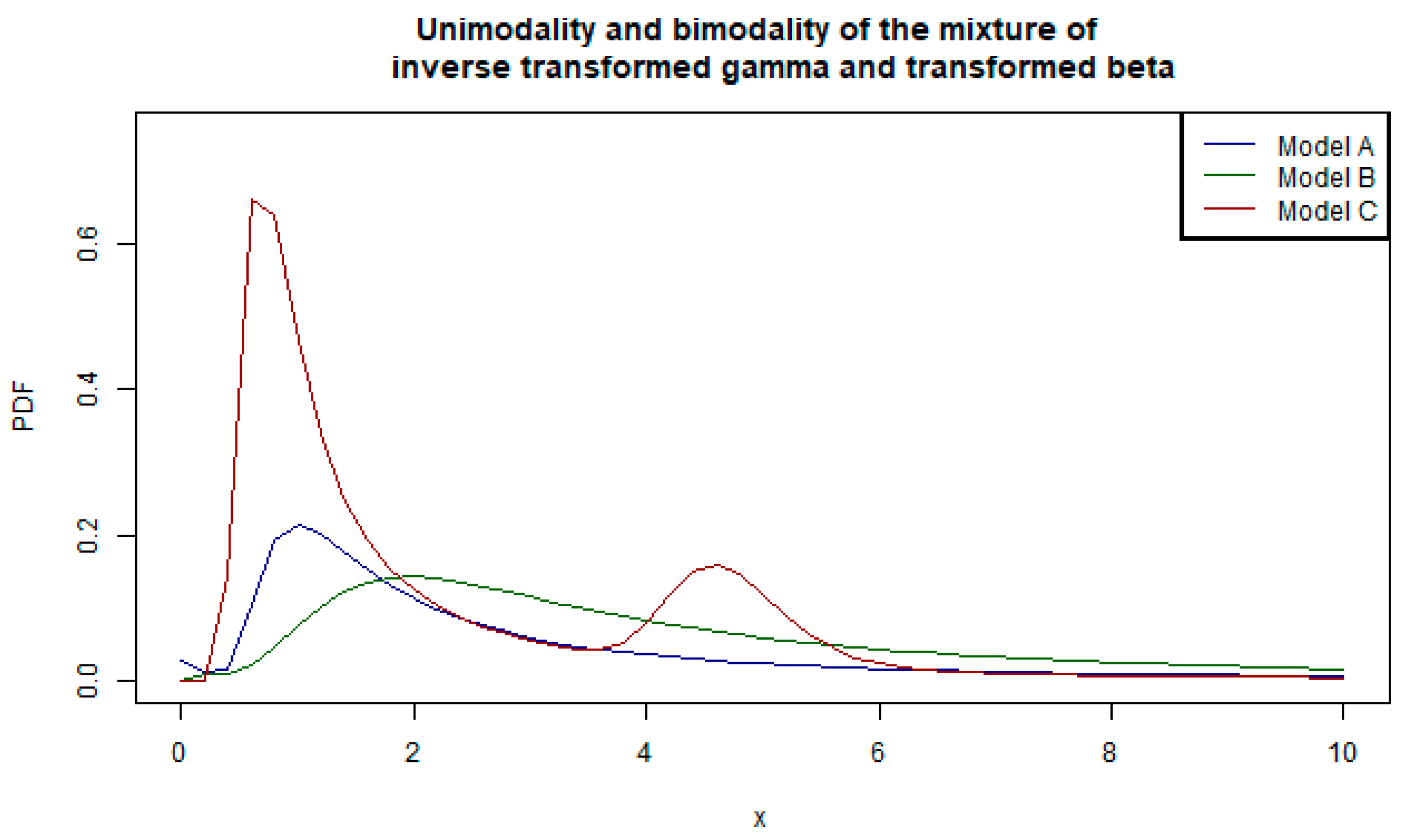
Figure 1. The pdfs of the two-component inverse transformed gamma and transformed beta mixture for different parameters.
Mathematics 12 00335 g001
Figure 2. The pdfs of the two-component Burr mixture for different parameters.
Mathematics 12 00335 g002
Figure 3. Boxplots of the taxi claims and the Danish loss data.
Mathematics 12 00335 g003
Figure 4. Histograms of the taxi claims and the Danish loss data.
Mathematics 12 00335 g004
Figure 5. Mean excess plots of the taxi claims and the Danish loss data.
Mathematics 12 00335 g005
Table 1. Parameter estimates corresponding to the models in Figure 1.
ϕ ϑ 1 ϑ 2
Model A ϕ = 1 α = 0.5 ,   τ = 2 ,   θ = 1 α = 0.1 ,   γ = 0.5 ,   τ = 2 ,   θ = 1
Model B ϕ = 2.5 α = 0.1 ,   τ = 0.5 ,   θ = 1 α = 0.9 ,   γ = 1.5 ,   τ = 5 ,   θ = 1
Model C ϕ = 5 α = 10 ,   τ = 3 ,   θ = 10 α = 0.2 ,   γ = 5 ,   τ = 2   , θ = 0.5
Table 2. Parameter estimates corresponding to the models in Figure 2.
ϕ ϑ 1 ϑ 2
Model A ϕ = 1 α = 0.1 ,   γ = 2 , θ = 1 α = 2 ,   γ = 5 , θ = 1
Model B ϕ = 2 α = 2 ,   γ = 0.6 , θ = 1 α = 3 ,   γ = 0.2 , θ = 1
Model C ϕ = 1 α = 10 ,   γ = 10 , θ = 3 α = 2.5 ,   γ = 8 , θ = 8
Table 3. Descriptive statistics of the South African taxi claims data.
Minimum Quantiles MeanMaximumStandard
Deviation
Coefficient of Variation SkewnessKurtosis
0.1(20.8, 45, 120.8)132.34803.3284.15632.156.47463.64
Table 4. Descriptive statistics of the Danish fire loss data.
Minimum Quantiles MeanMaximumStandard Deviation Coefficient of Variation SkewnessKurtosis
0.3134(1.1572, 1.6339, 2.6455)3.0627263.25047.9767032.6019.896549.5736
Table 5. Summary of the information criteria of the top 20 composite models for taxi claims (based on the BIC).
HeadTailpNLLAICBIC
GammaWeibull4270,197.8540,403.6540,438.8
ParalogisticInverse Gaussian4270,198.1540,404.2540,439.3
LoglogisticInverse Gaussian4270,200.7540,409.5540,444.6
ParalogisticWeibull4270,201.2540,410.5540,445.6
Inverse paralogisticInverse Gaussian4270,217.0540,442.1540,447.2
WeibullWeibull4270,202.4540,412.8540,447.9
GammaBurr5270,197.8540,405.6540,449.5
LoglogisticWeibull4270,204.4540,416.8540,452.0
ParalogisticBurr5270,201.1540,412.5540,456.4
WeibullBurr5270,202.4540,414.8540,458.7
Inverse BurrWeibull5270,202.5540,415.1540,459.0
LoglogisticBurr5270,204.4540,418.8540,462.7
Inverse BurrBurr6270,201.2540,417.1540,469.8
Inverse paralogisticWeibull4270,223.4540,454.7540,489.9
Inverse paralogisticBurr5270,223.4540,456.8540,500.7
BurrPareto5270,246.1540,502.3540,546.2
WeibullLognormal4270,259.9540,527.8540,562.9
GammaLognormal4270,260540,528.8540,563.9
GammaGeneralised Pareto5270,257.0540,524.0540,567.9
ParalogisticLognormal4270,262.9540,533.9540,569.0
Table 6. Summary of the empirical risk estimates, risk measures of the top 20 composite models for taxi claims data, and the percentage deviation with respect to the empirical risk estimates in parenthesis.
V a R 0.95 V a R 0.99 T V a R 0.95 T V a R 0.99
Empirical Estimates525.15091396.9011085.5832206.203
Parametric
HeadTail
GammaWeibull521.76 (−0.6%)1396.27 (0.0%)1125.77 (3.7%)2422.04 (9.8%)
ParalogisticInverse Gaussian547.96 (4.3%)1361.21 (−2.6%)1068.6 (−1.6%)2055.10 (−6.8%)
LoglogisticInverse Gaussian547.84 (4.3%)1361.62 (−2.5%)1068.80 (−1.5%)2056.09 (−6.8%)
ParalogisticWeibull521.92 (−0.6%)1394.70 (−0.2%)1124.46 (3.6%)2416.23 (9.5%)
Inverse paralogisticInverse Gaussian547.38 (4.2%)1363.79 (−2.4%)1070.18 (−1.4%)2061.91 (−6.5%)
WeibullWeibull522.21 (−0.6%)1389.41 (−0.5%)1119.77 (3.1%)2396.8 (8.6%)
GammaBurr521.78 (−0.6%)1396.5 (0.0%)1126.1 (3.7%)2423.17 (9.8%)
LoglogisticWeibull521.62 (−0.7%)1393.86 (−0.2%)1123.85 (3.5%)2415.2 (9.5%)
Paralogistic Burr521.92 (−0.6%)1394.71 (−0.2%)1124.46 (3.6%)2416.26 (9.5%)
WeibullBurr----
Inverse BurrWeibull522.15 (−0.6%)1395.0 (−0.1%)1124.66 (3.6%)2416.12 (9.5%)
LoglogisticBurr----
Inverse BurrBurr521.91 (−0.6%)1394.08 (−0.2%)1123.92 (3.5%)2414.26 (9.4%)
Inverse paralogisticWeibull520.81 (−0.8%)1393.196 (−0.3%)1123.73 (3.5%)2418.417 (9.6%)
Inverse paralogisticBurr521.06 (−0.8%)1394.12 (−0.2%)1124.48 (3.6%)2420.34 (9.7%)
BurrPareto532.21 (1.3%)1334.65 (−4.5%)1112.35 (2.5%)2391.68 (8.4%)
WeibullLognormal516.02 (−1.7%)1513.17 (8.3%)1270.78 (17.1%)3067.21 (39.0%)
GammaLognormal516.54 (−1.6%)1524.43 (9.1%)1286.50 (18.5%)3133.02 (42.0%)
GammaGeneralised Pareto585.11 (11.4%)1587.63 (13.7%)1396.13 (28.6%)3404.88 (54.3%)
ParalogisticLognormal513.46 (−2.2%)1511.45 (8.2%)1274.91 (17.4%)3098.64 (40.5%)
Table 7. Summary of the information criteria of the top 20 mixture models for taxi claims data (based on the BIC).
First ComponentSecond ComponentpNLLAICBIC
Inverse gammaLognormal5270,142.25540,294.5540,338.4
Inverse Gaussian Lognormal5270,142.45540,294.91540,338.81
Generalised ParetoLognormal6270,142.17540,296.35540,349.03
Inverse paralogisticLognormal5270,148.17540,306.35540,350.25
Inverse WeibullLognormal5270,148.29540,306.58540,350.48
Inverse BurrLognormal6270,146.59540,305.17540,357.85
LoglogisticLognormal5270,158.197540,326.39540,370.29
BurrLognormal6270,155.86540,323.72540,376.4
GammaLognormal5270,164.59540,339.19540,383.09
ParalogisticLognormal5270,167.79540,345.59540,389.49
LognormalWeibull5270,186.3540,382.6540,426.5
LoglogisticGeneralised Pareto6270,225.71540,463.43540,516.11
Generalised ParetoParalogistic6270,227.97540,467.94540,520.62
LoglogisticParalogistic5270,239.59540,489.17540,533.07
BurrLoglogistic6270,236.85540,485.70540,538.38
ParalogisticParalogistic5270,247.06540,504.11540,548.01
BurrBurr7270,236.71540,487.43540,548.89
Inverse gamma Paralogistic5270,248.70540,507.41540,551.31
Inverse gammaGeneralised Pareto6270,243.88540,499.75540,552.43
ParalogisticBurr6270,246.83540,505.67540,558.35
Table 8. Summary of the empirical risk estimates, risk measures of the top 20 mixture models for the taxi claims data, and the percentage deviation with respect to the empirical risk estimates in parenthesis.
V a R 0.95 V a R 0.99 T V a R 0.95 T V a R 0.99
Empirical Estimates 525.15091396.9011085.5832206.203
Parametric
First ComponentSecond Component
Inverse gammaLognormal513.98 (−2.1%)1382.65 (−1.0%)1142.3 (5.2%)2558.96 (16.0%)
Inverse GaussianLognormal514.55 (−2.0%)1373.99 (−1.6%)1134.85 (4.5%)2529.36 (14.6%)
Generalised ParetoLognormal514.63 (−2.0%)1383.4 (−1.0%)1142.86 (5.3%)2558.81 (16.0%)
Inverse paralogisticLognormal515.07 (−1.9%)1390.59 (−0.5%)1149.02 (5.8%)2580.52 (17.0%)
Inverse WeibullLognormal510.55 (−2.8%)1378.04 (−1.4%)1139.31 (4.9%)2560.72 (16.1%)
Inverse BurrLognormal513.78 (−2.2%)1389.68 (−0.5%)1148.59 (5.8%)2583.77 (17.1%)
LoglogisticLognormal517.67 (−1.4%)1391.51 (−0.4%)1149.05 (5.8%)2570.78 (16.5%)
BurrLognormal516.78 (−1.6%)1400.85 (0.3%)1157.8 (6.7%)2607.82 (18.2%)
GammaLognormal513.25 (−2.3%)1360.23 (−2.6%)1123.05 (3.5%)2489.42 (12.8%)
ParalogisticLognormal516.78 (−1.6%)1373.68 (−1.7%)1133.63 (4.4%)2515.69 (14.0%)
LognormalWeibull512.52 (−2.4%)1342.93 (−3.9%)1107.41 (2.0%)2431.57 (10.2%)
LoglogisticGeneralised Pareto518.2 (−1.3%)1349.01 (−3.4%)1157.27 (6.6%)2664.54 (20.8%)
Generalised ParetoParalogistic511.48 (−2.6%)1363.65 (−2.4%)1190.45 (9.7%)2846.36 (29.0%)
LoglogisticParalogistic513.22 (−2.3%)1372.25 (−1.8%)1223.63 (12.7%)3002.93 (36.1%)
BurrLoglogistic515.45 (−1.8%)1351.42 (−3.3%)1181.42 (8.8%)2799.21 (26.9%)
ParalogisticParalogistic507.18 (−3.4%)1384.18 (−0.9%)1255.56 (15.7%)3176.84 (44.0%)
BurrBurr516.17 (−1.7%)1351.72 (−3.2%)1181.84 (8.9%)2798.08 (26.8%)
Inverse gammaParalogistic504.42 (−3.9%)1436.60 (2.8%)1327.5 (22.3%)3496.71 (58.5%)
Inverse gammaGeneralised Pareto507.28 (−3.4%)1402.21 (0.4%)1268.23 (16.8%)3220.81 (46.0%)
ParalogisticBurr507.44 (−3.4%)1376.18 (−1.5%)1240.94 (14.3%)3109.60 (40.9%)
Table 9. Summary of the information criteria of the top 20 composite models for Danish fire loss data (based on the BIC)—these results are similar to those reported in Grün and Miljkovic [8].
HeadTailpNLLAICBIC
WeibullInverse Weibull43820.017648.027671.30
ParalogisticInverse Weibull43820.147648.287671.56
Inverse BurrInverse Weibull53816.347642.687671.79
WeibullInverse paralogistic43820.937649.877673.15
Inverse BurrInverse paralogistic53817.077644.147673.25
ParalogisticInverse paralogistic43821.047650.087673.36
WeibullLoglogistic43821.237650.467673.74
Inverse BurrLoglogistic53817.377644.747673.85
ParalogisticLoglogistic43821.327650.657673.93
LoglogisticInverse Weibull43821.387650.767674.04
WeibullBurr53817.577645.147674.24
ParalogisticBurr53817.727645.437674.54
Inverse BurrBurr63814.007639.997674.92
LoglogisticInverse paralogistic43822.157652.317675.59
Inverse BurrInverse gamma53818.307646.617675.71
ParalogisticInverse gamma43822.227652.437675.72
LoglogisticLoglogistic43822.417652.827676.10
WeibullParalogistic43822.447652.887676.17
ParalogisticParalogistic43822.537653.057676.34
Inverse BurrParalogistic53818.687647.377676.47
Table 10. Summary of the empirical risk estimates, the risk measures of the top 20 composite models for Danish fire loss data (reported in Grün and Miljkovic [8]) and the percentage deviation with respect to the empirical risk estimates in parenthesis.
V a R 0.95 V a R 0.99 T V a R 0.95 T V a R 0.99
Empirical Estimates8.40629824.6137822.1550954.60396
Parametric
HeadTail
WeibullInverse Weibull8.02 (−4.6%)22.77 (−7.5%)22.64 (2.2%)63.86 (17.0%)
ParalogisticInverse Weibull8.02 (−4.6%)22.79 (−7.4%)22.67 (2.3%)64.00 (17.2%)
Inverse BurrInverse Weibull8.01 (−4.7%)22.73 (−7.7%)22.59 (2.0%)63.67 (16.6%)
WeibullInverse paralogistic8.03 (−4.5%)22.64 (−8.0%)22.38 (1.0%)62.65 (14.7%)
Inverse BurrInverse paralogistic8.03 (−4.5%)22.65 (−8.0%)22.39 (1.1%)62.69 (14.8%)
ParalogisticInverse paralogistic8.03 (−4.5%)22.68 (−7.9%)22.44 (1.3%)62.89 (15.2%)
WeibullLoglogistic8.05 (−4.2%)22.7 (−7.8%)22.43 (1.2%)62.8 (15.0%)
Inverse BurrLoglogistic8.04 (−4.4%)22.64 (−8.0%)22.35 (0.9%)62.46 (14.4%)
ParalogisticLoglogistic8.05 (−4.2%)22.71 (−7.7%)22.46 (1.4%)62.89 (15.2%)
LoglogisticInverse Weibull8.05 (−4.2%)22.96 (−6.7%)22.93 (3.5%)65.02 (19.1%)
WeibullBurr8.22 (−2.2%)25.18 (2.3%)26.98 (21.8%)82.59 (51.3%)
ParalogisticBurr8.22 (−2.2%)25.18 (2.3%)26.98 (21.8%)82.61 (51.3%)
Inverse BurrBurr8.22 (−2.2%)25.13 (2.1%)26.88 (21.3%)82.15 (50.4%)
LoglogisticInverse paralogistic8.05 (−4.2%)22.79 (−7.4%)22.6 (2.0%)63.55 (16.4%)
Inverse BurrInverse gamma8.1 (−3.6%)22.33 (−9.3%)21.42 (−3.3%)57.83 (5.9%)
ParalogisticInverse gamma8.11 (−3.5%)22.44 (−8.8%)21.57 (−2.6%)58.48 (7.1%)
LoglogisticLoglogistic8.06 (−4.1%)22.82 (−7.3%)22.61 (2.1%)63.52 (16.3%)
WeibullParalogistic8.11 (−3.5%)22.6 (−8.2%)21.98 (−0.8%)60.35 (10.5%)
ParalogisticParalogistic8.11 (−3.5%)22.62 (−8.1%)21.99 (−0.7%)60.41 (10.6%)
Inverse BurrParalogistic8.1 (−3.6%)22.47 (−8.7%)21.78 (−1.7%)59.52 (9.0%)
Table 11. Summary of the information criteria of the top 20 mixture models for Danish fire loss data (based on the BIC).
First ComponentSecond ComponentpNLLAICBIC
BurrBurr73786.477586.957627.69
Inverse WeibullBurr63790.617593.227628.15
LoglogisticBurr63791.607595.207630.13
Inverse paralogisticBurr63792.027596.037630.96
ParalogisticBurr63794.367600.727635.64
Inverse BurrBurr73790.737595.467636.21
GammaBurr63798.0047608.017642.93
LognormalBurr63799.067610.127645.05
Generalised ParetoBurr73797.917609.837650.57
Inverse GaussianBurr63801.977615.947650.86
Inverse gammaBurr63803.797619.577654.5
Inverse exponentialBurr53810.037630.067659.17
ExponentialBurr53811.327632.637661.74
Inverse ParetoBurr63810.067632.127667.04
WeibullBurr63810.827633.657668.57
ParetoBurr63811.337634.657669.58
Inverse WeibullInverse Burr63833.767679.537714.45
Inverse paralogistic Inverse Weibull53840.247690.497719.59
Inverse WeibullInverse gamma53840.537691.077720.17
Inverse BurrInverse Burr73833.797681.577722.32
Table 12. Summary of the empirical risk estimates, the risk measures of the top 20 mixture models for Danish fire loss data and the percentage deviation with respect to the empirical risk estimates in parenthesis.
V a R 0.95 V a R 0.99 T V a R 0.95 T V a R 0.99
Empirical Estimates 8.40629824.6137822.1550954.60396
Parametric
First ComponentSecond Component
BurrBurr8.26 (−1.7%)27.0 (9.7%)34.74 (56.8%)119.72 (119.3%)
Inverse WeibullBurr8.19 (−2.6%)25.23 (2.5%)27.21 (22.8%)83.83 (53.5%)
LoglogisticBurr9.245 (10.0%)36.07 (46.5%)60.00 (170.8%)234.13 (328.8%)
Inverse paralogisticBurr8.2025 (−2.4%)25.32 (2.9%)27.37 (23.5%)84.498 (54.7%)
Inverse BurrBurr8.1902 (−2.6%)25.23 (2.5%)27.22 (22.9%)83.87 (53.6%)
GammaBurr9.395 (11.8%)36.48 (48.2%)59.80 (169.9%)232.22 (325.3%)
Inverse GaussianBurr8.59 (2.2%)31.88 (29.5%)46.53 (110.0%)172.91 (216.7%)
LognormalBurr8.71 (3.6%)32.67 (32.7%)48.82 (120.4%)183.18 (235.5%)
Generalised ParetoBurr8.81 (4.8%)33.31 (35.3%)50.72 (128.9%)191.77 (251.2%)
Inverse gammaBurr9.14 (8.7%)32.64 (32.6%)43.71 (97.3%)156.09 (185.9%)
Inverse exponentialBurr9.61 (14.3%)34.555 (40.4%)--
ExponentialBurr9.51 (13.1%)33.85 (37.5%)45.41 (105.0%)162.22 (197.1%)
Inverse ParetoBurr9.61 (14.3%)34.55 (40.4%)--
ParalogisticBurr8.43 (0.3%)26.85 (9.1%)30.07 (35.7%)95.73 (75.3%)
WeibullBurr8.44 (0.4%)26.89 (9.2%)30.14 (36.0%)96.04 (75.9%)
ParetoBurr9.51 (13.1%)33.85 (37.5%)45.39 (104.9%)162.15 (197.0%)
Inverse WeibullInverse Burr8.15 (−3.0%)21.51 (−12.6%)20.11 (−9.2%)51.88 (−5.0%)
Inverse paralogistic Inverse Weibull8.13 (−3.3%)19.92 (−19.1%)17.89 (−19.3%)42.34 (−22.5%)
Inverse WeibullInverse gamma8.53 (1.5%)22.16 (−10.0%)19.84 (−10.4%)48.35 (−11.5%)
Inverse BurrInverse Burr8.15 (−3.0%)21.49 (−12.7%)20.096 (−9.3%)51.83 (−5.1%)
Disclaimer/Publisher’s Note: The statements, opinions and data contained in all publications are solely those of the individual author(s) and contributor(s) and not of MDPI and/or the editor(s). MDPI and/or the editor(s) disclaim responsibility for any injury to people or property resulting from any ideas, methods, instructions or products referred to in the content.

