Abstract
A recent development in Fault Tree Analysis (FTA), known as Dynamic and Dependent Tree Theory (D2T2), accounts for dependencies between the basic events, making FTA more powerful. The method uses an integrated combination of Binary Decision Diagrams (BDDs), Stochastic Petri Nets (SPN) and Markov models. Current algorithms enable the prediction of the system failure probability and failure frequency. This paper proposes methods which extend the current capability of the D2T2 framework to calculate component importance measures. Birnbaum’s measure of importance, the Criticality measure of importance, the Risk Achievement Worth (RAW) measure of importance and the Risk Reduction Worth (RRW) measure of importance are considered. This adds a vital ability to the framework, enabling the influence that components have on system failure to be determined and the most effective means of improving system performance to be identified. The algorithms for calculating each measure of importance are described and demonstrated using a pressure vessel cooling system.
Keywords:
system failure modelling; dependent failures; system unavailability assessment; dynamic and dependent tree theory MSC:
60H30
1. Introduction
Risk assessment is commonly performed on safety-critical systems to ensure that their performance meets the required standard [1]. This involves calculating the likelihood or frequency that systems fail in critical modes, which can kill or injure people. Fault tree analysis is the most common method used in the industry to perform this task. Traditional Fault Tree Analysis (FTA), known as Kinetic Tree Theory (KTT), was derived by Vesely [2] in 1970 to assess the failure of engineering systems. The tree structure provides a clear visual representation of the causes of system failure in terms of basic events such as component failures, software failures and human errors. Engineers are familiar with this form of causality diagram, which enables easy peer review and regulator assessment. The subsequent two-stage analysis delivers the minimal cuts sets, i.e., the necessary and sufficient combinations of basic events which cause system failure, along with the system failure probability, the system failure frequency, and measures of importance. Importance measures determine the contribution of each component or minimal cut set to system failure and provide a means to identify weaknesses that can be targeted to improve overall system performance [3,4,5]. Different importance measures consider different factors in their definition and can account for the vulnerability of the system in terms of failure when a component fails (the inclusion of redundancy that needs several components to fail to cause system failure), the frequency by which a component fails and the speed at which a repair back to functioning condition can be achieved.
One limitation of KTT is its requirement to employ approximations. If the fault tree structure produces a large number of minimal cut sets, it may not be possible to obtain them all, in which case, a culling approach is adopted to obtain the most significant combinations [6,7]. Approximations, such as the Rare Event Approximation or the Minimal Cut Set Upper Bound, are also used during the quantification stage since full inclusion–exclusion expansion cannot be evaluated [3]. The development of Binary Decision Diagram (BDD) methods in the 1990s and the subsequent research to efficiently convert the fault tree to BDDs overcame this limitation, enabling exact quantification to be performed [8,9,10,11,12,13,14].
There are, however, additional limitations of KTT, including the necessary assumption of independence between the basic events and, in many computer implementations, the requirement for constant component failure and repair rates. The models that calculate component failure probabilities usually apply to components that are non-repairable or experience revealed or unrevealed failures. These are also very limited in terms of their ability to represent the maintenance strategies employed in a system. Increasing failure rates are encountered when components experience wear-out. Furthermore, when failure does occur, repair is not a random process and, thus, it could be questioned if repair rates can ever be considered constant. The assumption of independence is extremely limiting and not appropriate for most modern engineering systems. Dependencies can occur in a variety of ways, for example, due to opportunistic maintenance, employing standby redundancy or considering common cause failures.
These restrictions limit the ability of KTT to model modern engineering systems effectively. Alternative approaches, such as Markov models [15] or Stochastic Petri Nets (SPN) [16,17], can be employed to overcome the assumptions. Whilst these methods can accommodate dependencies and, for SPNs, non-constant failure and repair rates are possible, both can be computationally demanding for even relatively simple systems. This is especially true for SPNs when modelling large systems whose failure events are rare. The large simulation times required to achieve convergence in the results often make the method impractical for real applications. Additionally, the tree structure is not retained, and thus, all the advantages of this causality form are lost. Approaches that address these issues and retain the tree structure have been developed, with the most advanced of these being Dynamic Fault Trees [18,19]. This approach allows dependencies and complexities to be incorporated into the model through the use of a SPARE (for spare or standby components) or a SEQ (for a sequence of events) gate, which are then analysed using a Markov model, and the results substituted back into the fault tree. However, the dependent events must all appear below a single gate. As such, if the dependent events are not all below the same gate, as for example when dependencies occur due to the maintenance process, this approach cannot be used.
In 2023, Andrews and Tolo [20] published the D2T2 methodology, which is designed specifically to address these limitations. The methodology retains the tree structure and combines the use of BDDs, along with Markov and SPN models, to analyse engineering systems featuring non-constant failure and repair rates, component dependencies, and complex maintenance strategies as efficiently as possible. The methodology ensures that no matter how far apart the dependent events are in the tree structure, the dependency model features only these components. As such, the dependency models are minimal, maximising efficiency. The methodology enables the calculation of both the system failure probability and the system failure frequency. However, in order to obtain the full range of outputs, the methodology needs to be extended to calculate commonly used measures of importance. This paper considers measures of component importance relating to the top event probability, including Birnbaum’s measure of importance [21], the Criticality Measure of Importance [22], the Risk Achievement Worth (RAW) and the Risk Reduction Worth (RRW) [23].
2. D2T2 Methodology
In 2023, Andrews and Tolo proposed the D2T2 methodology. It provides a holistic generalised approach to model systems with complexities, including components with non-constant failure/repair rates, dependencies between component failures, complex maintenance processes, and event sequences. The methodology retains the fault tree structure to provide a clear representation of the system failure causality and combines the use of the BDD analysis with Markov and SPNs to model dependencies and complexities as efficiently as possible.
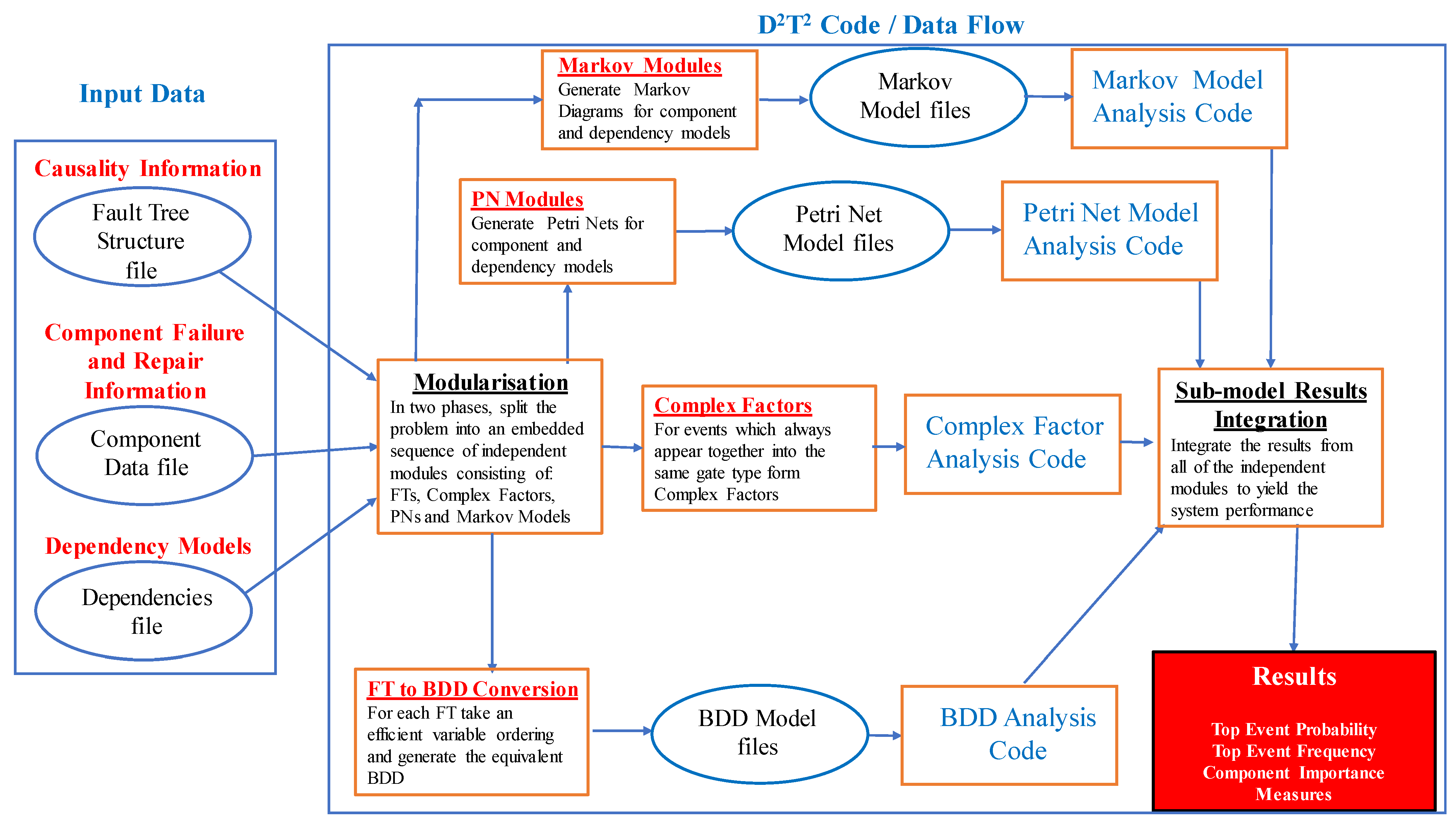
The methodology begins by manipulating the fault tree such that it can be reduced to a series of independent modules each of which can be solved using the appropriate approach. The results obtained are then integrated to obtain the top event probability and system failure frequency. D2T2 employs modified versions of two of the most effective modularisation approaches: the reduction algorithm used in FAUNET [24,25] and the Linear Time algorithm of Dutuit and Rauzy [26]. Due to the different philosophies taken by the two methods, they can be applied sequentially to achieve an improved degree of modularisation than either can achieve in isolation. These methods identify independent sub-trees to enable the efficient solution of conventional FTA. In their original form, they account for dependencies introduced through basic events that occur more than once in the fault tree structure. The changes incorporated in these approaches extend their capability, enabling dependencies to exist between different basic events. When the modularization process is complete, the fault tree will be represented as a number of concise independent modules, which will be solved separately. The algorithm then utilises Markov or Petri net models to solve each dynamic, dependent, or complex part of the problem. Those modules which retain the fault tree form are converted to a BDD for analysis using an effective variable ordering scheme. Finally, the results from the analysis of the independent Markov, Petri net, complex factors, and components are used to quantify the BDD models, calculating the top event probability and the system failure frequency. Figure 1 summarises this process. The objective of the work contained in this paper is to extend the analysis framework to include component importance measures.
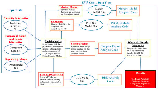
Figure 1.
The D2T2 solution process.
3. Pressure Vessel Cooling System Case Study
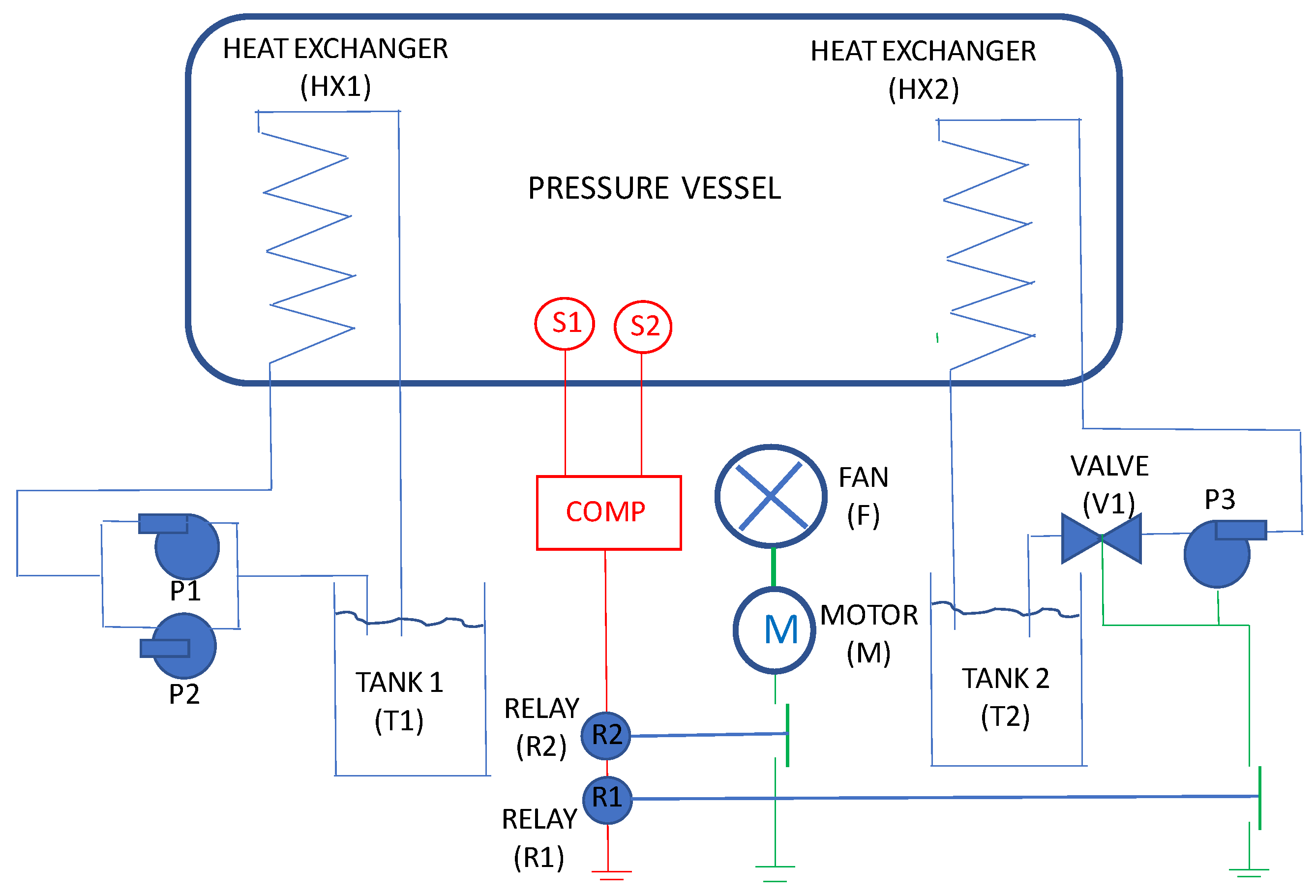
To illustrate the calculation processes needed to deliver the importance measures for fault trees evaluated using the D2T2 methodology, a pressure vessel cooling system will be used. The details of this example and its analysis are given in [20]. A schematic of the system is shown in Figure 2. The system features four sub-systems: a primary cooling system, a temperature detection system, a fan cooling system and a secondary cooling system. If the primary cooling system fails, then the vessel temperature will increase. An increase in vessel temperature will be detected by the sensing system, which will close relays, activating both the fan cooling system and the secondary cooling system. The component failure events considered in the analysis are given in Table 1. The fault tree has then been constructed for causes of the cooling system failure that will require the primary cooling system to fail along with any of the temperature sensing systems: the fan cooling system and the secondary cooling system.
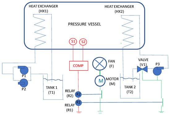
Figure 2.
Pressure vessel cooling system.

Table 1.
Basic event definitions.
The essential details of the system analysis to be used in the importance measures calculations are given in the following sections. The fault tree for the failure of this cooling system is shown in Figure 3. The form of the fault tree presented has been contracted into an alternating sequence of AND and OR gates. The complexity and dependency details, which are the reasons that solutions cannot be achieved through traditional FTA, are given in Table 2.

Figure 3.
Pressure vessel cooling system failure fault tree.

Table 2.
Complexity and dependency group details.
3.1. Fault Tree Modularisation
As shown in Figure 1, the data input to the D2T2 methodology take the form of a fault tree structure file (defining the fault tree in Figure 3), the component failure and repair data, and the dependency models (Petri net and Markov models for the dependencies defined in Table 3). In order to show how the importance measures are calculated, it is necessary to describe some aspects of the D2T2 methodology. The modularisation process is essential for the importance measures calculation and so will be explained in detail in this section. The first task of the D2T2 methodology is to reduce the problem to a sequence of independent sub-problems, which is accomplished by the modularisation algorithms. It is these modules that are to be used to then calculate the importance measures, as such, they will be developed stage by stage.

Table 3.
Details of the complex factors.
Application of Modified FAUNET Reduction Algorithm
The original reduction algorithm [24,25] repeatedly applies three processes to the fault tree known as: contraction, factorisation and extraction.
Contraction: compresses the structure into an alternating sequence of AND and OR gates.
Factorisation: defines factors in the tree where the events always appear together entering the same gate type. For analyses performed using D2T2, it is necessary to modify this requirement to account for the dependencies between the basic events, and so the factors additionally need to contain only independent initiating events, independent enabling events, or all of the events that belong to a dependency group.
Extraction: re-arranges the fault tree sub-structures where an AND (OR) gate develops into OR (AND) gates that all have X as an input, to extract the factor, X, such that one of the following mappings take place:
For the pressure vessel cooling system fault tree shown in Figure 3, the first contraction stage has already been applied so it exists as an alternating sequence of AND and OR gates.
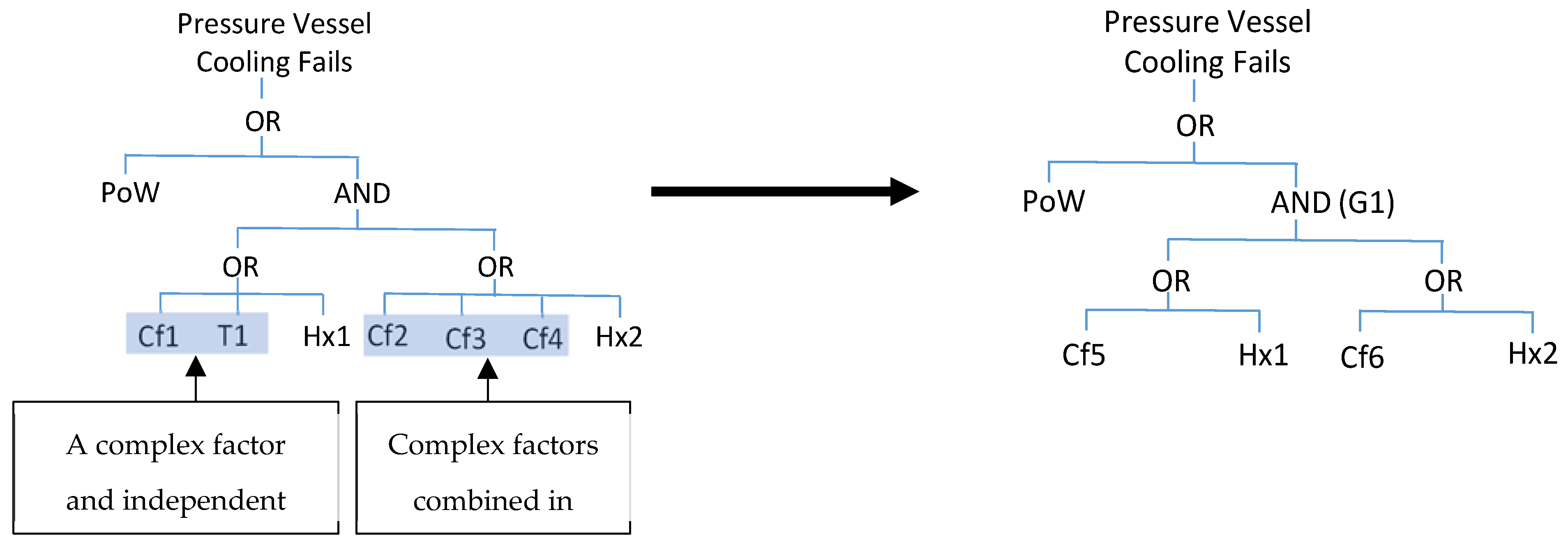
The application of the first factorisation process identifies four factors Cf1–Cf4, as shown in Figure 4.

Figure 4.
Factorisation Stage 1 application.
The repeated event PoW then enables a restructuring of the fault tree using the first mapping in Equation (1) to extract this event to a higher level. The result of this is shown in Figure 5. Since it is already an alternating sequence of AND and OR gates, the execution of contraction stage 2 produces no changes.

Figure 5.
Extraction Stage 1 application.
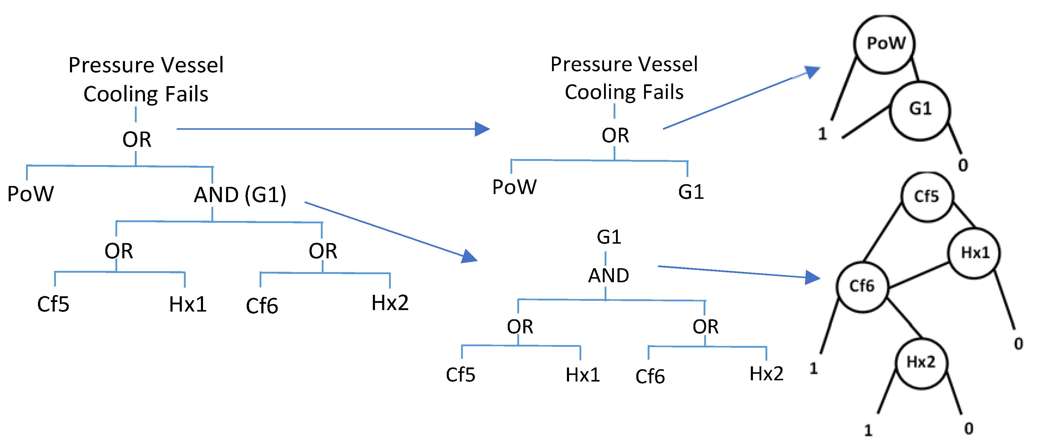
Applying the factorisation stage for a second time produces two new factors: Cf5 = CF1 + T1 and CF6 = Cf2 + Cf3 + Cf4 (See Figure 6). Further use of the contraction, factorisation or extraction processes result in no changes to the fault tree, and its form at the end of the reduction modularisation is shown on the left hand side of Figure 7.
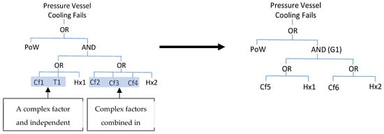
Figure 6.
Final factorisation phase.
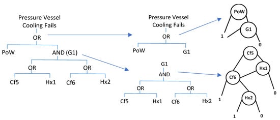
Figure 7.
Application of the linear time algorithm.
The linear time algorithm [26] identifies independent gates in the fault tree structure and can be applied to produce a further reduction in the size of the fault tree to be analysed. Only a minor modification in the labelling is necessary for this to work for dependencies between basic events. All events in any dependency group are labelled with the dependency group label. Applying the algorithm to the final fault tree resulting from the reduction modularisation, identifies that the TOP gate and the gate labelled G1 are both independent of the rest of the structure and these two sections can be analysed separately to simplify the quantification process (Figure 7). Both fault tree modules will be converted to BDDs using the ordering for the tree headed G1 and for the tree for the TOP event. It should be noted that the fault tree section headed G1 contains basic events Hx1 and Hx2, which feature a dependency solved using a Petri Net and the results are substituted into the analysis of this BDD. TOP contains only independent events and, therefore, its solution proceeds as for BDDs of conventional fault trees.
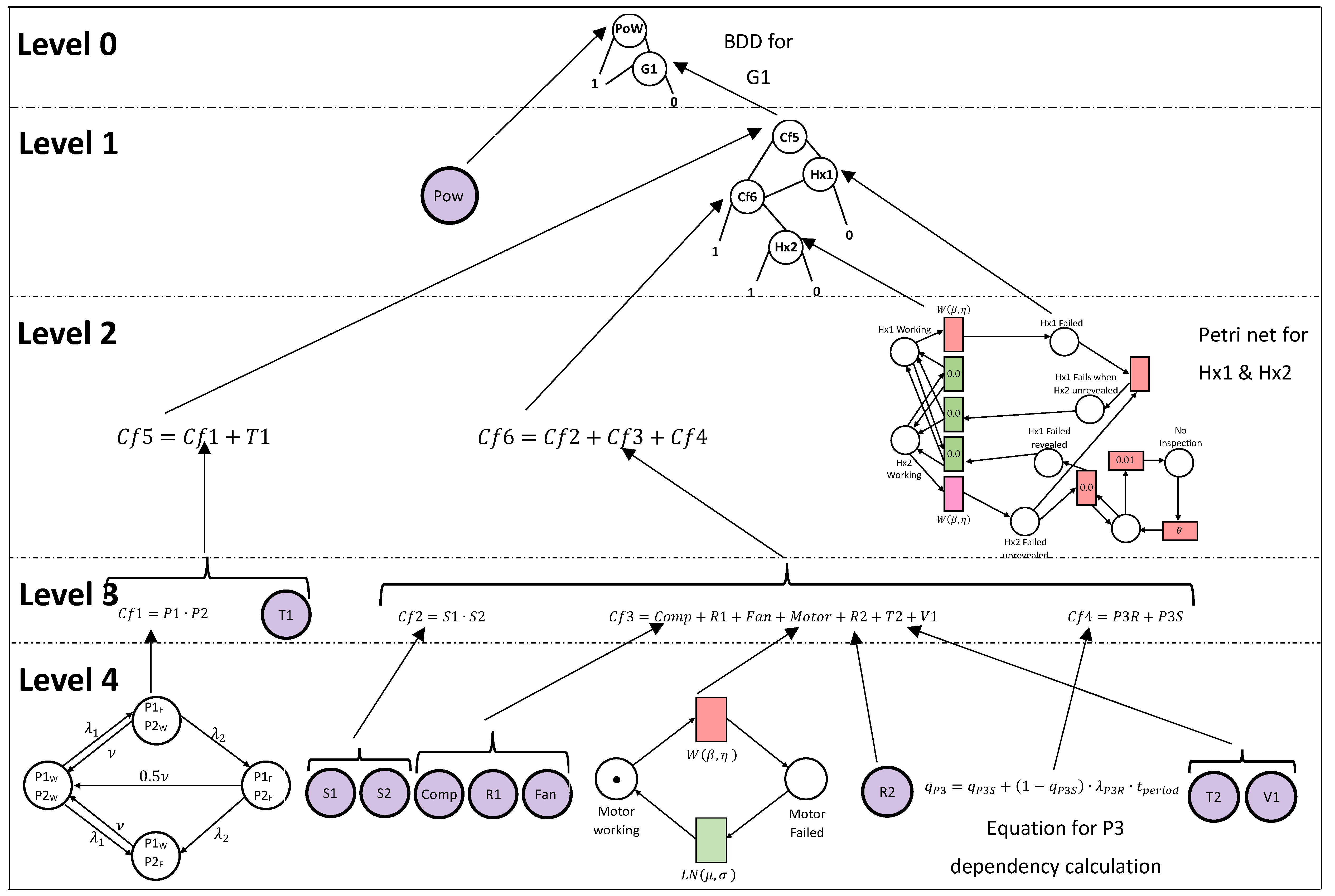
At the end of the modularisation process of the D2T2 methodology, the problem has been redefined to be the analysis of a series of smaller modules. Each module is independent of the rest of the analysis and can be solved separately. This results in a multi-layer analysis that culminates in the analysis of a final BDD model for the top gate of the original fault tree. The analysis of other BDDs, complex factors, Petri nets, Markov models and component failure probabilities all feed into this quantification process. The analysis structure is illustrated in Figure 8, with a summary of the complex factors given in Table 3.
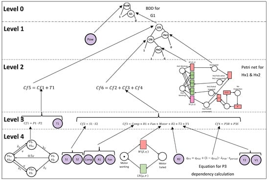
Figure 8.
Hierarchical Analysis Structure.
4. Importance Measures
When assessing a system, its performance is dependent upon that of its components. Certain components will play a more significant role in causing or contributing to system failure than others. The contribution that a component makes to system failure is known as its importance. The concept of importance was first introduced by Birnbaum in 1969 [21]; since this time, numerous measures of importance have been developed to assess the different roles that a component failure can play in the deterioration of system state. Measures of importance can be categorised as either deterministic or probabilistic and assign a value between 0 and 1 to each component, with 1 signifying the highest level of contribution. Deterministic measures of importance, such as the structural measures of importance [3], do not account for the reliability of the component(s). Probabilistic measures of importance take component failure probabilities and intensities into account and are, therefore, more useful than deterministic measures in practical reliability problems. Different measures are also relevant to the predicted system unavailability or unreliability. This paper focuses on those measures with relevance to the system unavailability: Birnbaum, Criticality [22], Risk Assessment Worth and Risk Reduction Worth [23]. Interpreting these importance measures enables weaknesses within the system to be identified and indicates where resources can be focused to improve system performance. It should be noted that another measure of importance relevant to the system unavailability is the Fussel–Vesely measure [27]. This measure requires the minimal cut sets to be calculated and, as such, is considered beyond the scope of this paper. The measures considered in this paper can be calculated directly from the fault tree structure without first deriving the minimal cut sets.
Each measure is defined below, and the equations given enable the measure to be quantified when all component failures are independent. These definitions will then be extended to consider the situation when dependencies occur in Section 5.
4.1. Birnbaum’s Measure of Importance
Birnbaum’s measure of importance, denoted by , also known as the Criticality Function, is defined as the probability that the system is in a critical state for component i. The system is in a critical state for component i if the state of the system components results in the system being in a working state, but should component fail, it causes the system to transition to the failed state. An expression for this measure is given in Equation (2):
where is the system unavailability function, the vector of component unavailability’s and
When the component failure probabilities are all independent, is linear in each , and an alternative expression for Equation (2) is as follows:
When a fault tree, where all basic events are independent, is converted to a BDD, Birnbaum’s measure of importance can be calculated via a single sweep of the BDD. For each component, , is given by where:
where is the probability of the path section from the root vertex to node , is the probability of the path section from the end of the 1-branch of node to a terminal node, is the probability of the path section from the end of the 0-branch of node to a terminal node, and is the probability of path k, which does not pass through node .
4.2. Criticality Measure of Importance
The criticality measure of importance for component is defined as the probability that the system is in a critical state for component and fails, weighted by the system’s unavailability at time . An expression for this measure when the basic event is independent of other component failures is given in Equation (5).
When component belongs to a dependency group, and will be dependent. Therefore, the calculation of the system being in a critical state for component and has failed will have to take this into consideration.
4.3. Risk Assessment Worth (RAW) and Risk Reduction Worth (RRW)
The Risk Achievement Worth (RAW) calculates the relative increase in system unavailability when it is known that component has failed. It can be calculated using Equation (6).
The Risk Reduction Worth (RRW) calculates the relative reduction in system unavailability when it is known that component is working. It is calculated using Equation (7).
Since all the terms in Equations (6) and (7) are calculated when predicting and Birnbaum’s measures of importance, it is a cheap process to provide these extra measures of importance.
5. Importance Measure Calculation Methodologies for Dependent Events
The following sections describe the methodologies to calculate each type of importance measure taking the modularised fault tree as the system failure model. The methods presented will enable the importance measures to be calculated when dependencies exist between the basic events. Each of the modules are mutually independent, as a consequence, any basic event will only feature in one of these modules or remain a single component model. In addition, any dependency will only feature in one module. In every case of the top event, the system failure model, will be represented via a BDD. BDDs emerging from the modularisation process can be classified as independent,, where all of the variables appearing on the diagram are independent of each other, or, as dependent, featuring some variables that have dependencies.
The function that represents system failure probability will be a function of probabilities taken from independent BDD modules, , j = 1, ……, N1, dependent BDD modules, , j = 1, ……, N2, Petri Net Modules, , j = 1, ……, N3, Markov modules, , j = 1, ……, N4, Complex Factor modules, Cfj, j = 1, ……, N5 and components. This is illustrated by the structure shown in Figure 8.
The calculation of each importance measure is discussed in terms of its contribution to system failure probability, accounting for the modularised system failure probability function.
5.1. Birnbaum’s Measure of Importance
Using Equation (2), Birnbaum’s measure of importance for any component can be evaluated from two system evaluations, one conditional on the component failed and the other conditional on the component working. From the example of modularisation shown in Figure 8, it can be seen that for every component failure event there is a single path leading up through the diagram to the top event. This path defines the modules whose probabilities are a function of the component failure probability. If N such modules appear directly on the path from the root basic event to the top event, then Birnbaum’s measure of importance can be evaluated for component i using the chain rule:
where is the probability that module Mj is in a critical state for module Mk. Evaluating Equation (8) requires the ability to calculate the criticality function for modules defined by complex factors, BDDs, PNs and Markov modules. The details of how these criticality functions are calculated for each situation is outlined below.
5.1.1. Independent Components Failures Modelled by Complex Factors
Complex factors will be of one logic gate type, AND or OR, linking combinations of either basic events or other complex factors. These combinations of events are either all independent or all belonging to a dependency group. In the case that the complex factor represents a dependency group, then the probability of the event combination will be determined from the associated Petri Net or Markov model. In the situation that the complex factor is defined by independent events, then the probability of the factor will be a linear function of the probabilities of its elements, and Equation (3) holds.
The following can be used for independent complex factors combining events with an OR gate:
where are basic events or other complex factors. The complex factor probability is then given as follows:
where qj is the probability of and:
For an independent complex factor that combines events with an AND operator:
and
5.1.2. Dependent Component Failures in a Markov Model
To calculate Birnbaum’s measure of importance for component j when j is in a dependency group analysed by a Markov model, it is necessary to return to the definition of the measure, i.e., the system is in a critical state for component such that the failure of component will cause the system to fail (Equation (2)). To evaluate the two conditional probabilities in Equation (2), the Markov state transition diagram can be examined, and the system states partitioned into those where the relevant component, j, has failed and those where the component is working. Amongst those states where j has failed, is evaluated by establishing the likelihoods of these states resulting in system failure. To calculate , the probability is the likelihood of the states where j is working, resulting in a system failed state. Using Equation (2) then gives:
where , j = 1, ……, NMKV, are the probabilities of the states on the Markov state transition diagram.
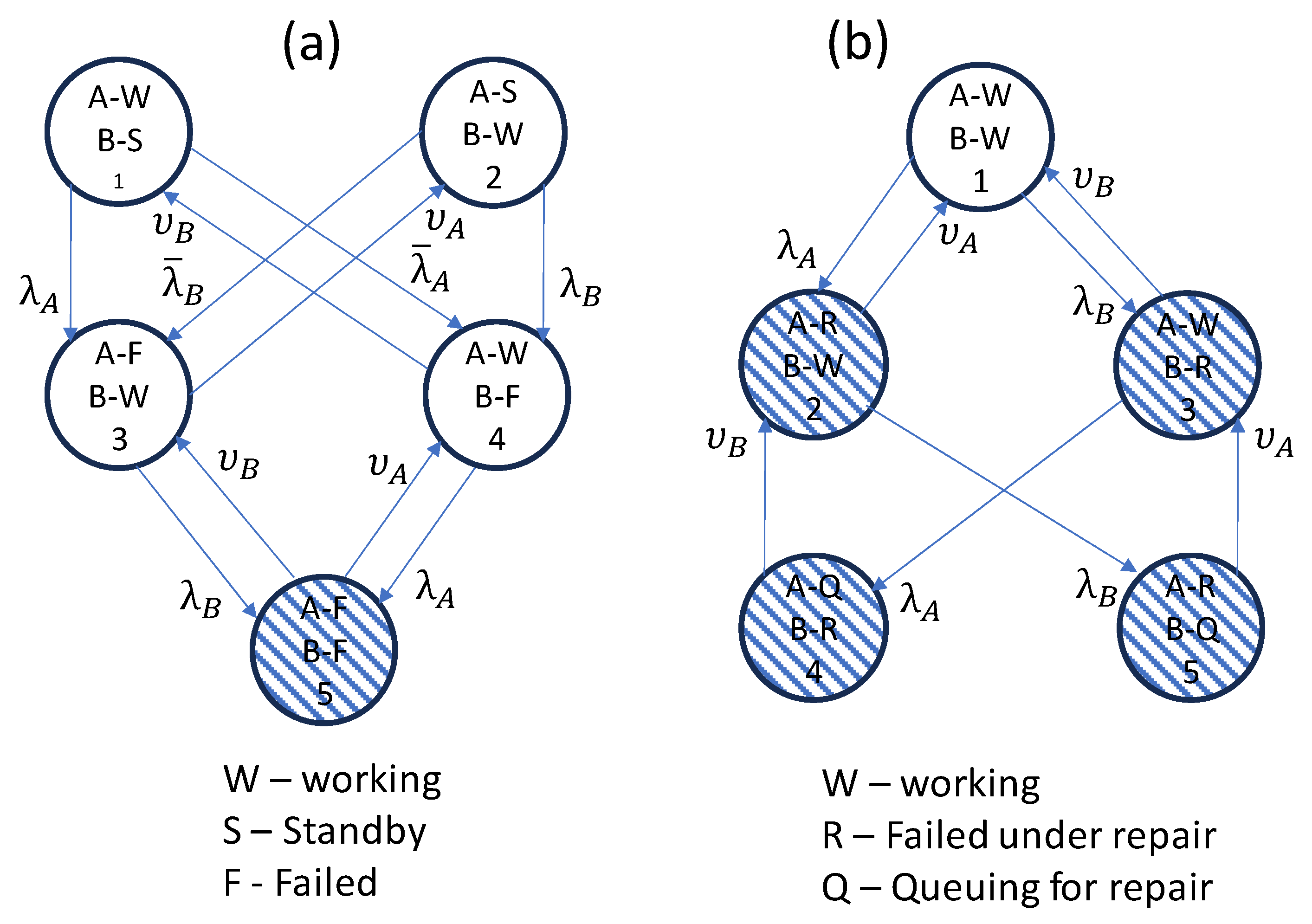
Markov models are used in the analysis to represent the dependencies between all the elements of a complex factor. As examples, consider the two situations where the Markov models are illustrated in Figure 9, both where the complex factor is dependent upon two components: A and B.
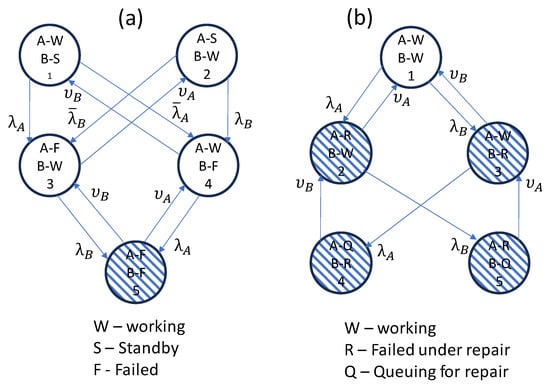
Figure 9.
(a) Markov model for a warm standby system; (b) Markov model in the case of one maintenance engineer (hatched states – system failure).
In the first case, the model represents a dependency due to components A and B operating in a warm standby configuration (Figure 9a). As such, the sub-system represented by the Markov model fails when both A and B have failed: . Consider first the criticality function for component A. For states 3 and 5, component A has failed, and for the remaining states, 1, 2 and 4, A is in a working state (i.e., working or in standby). Of the states with component A failed, state 5 has system failure. Therefore, the conditional probability that the system has failed given that component A has failed, . Since none of the states with A working result in system failure, . Repeating the process for component B gives:
In the second example, the dependency is a maintenance dependency between components A and B due to their shared repair engineer (Figure 9b). When one component has failed and the second component fails, it must queue until the engineer has completed the repair of the first component before the second component repair can start. The system in this case will fail if A OR B fails (under repair or queuing for repair), so . Partitioning the states for component A, states 2, 4 and 5 have A failed, and in states 1 and 3, A is working. States 2–5 represent those states where the system has failed. Therefore, and . Completing a similar process for component B gives the following:
5.1.3. Dependent Components Failed Modelled via Petri Net
When the dependency is modelled using a Petri net, the model structure is different to that of a Markov model, and the states represented in the places, in most cases, just refer to the status of a single component and are not mutually exclusive. Thus, during the simulation, the data are retained to enable the required predictions to be made. To calculate , the criticality function for component j data needs to be retained in order to calculate and . The total time that the simulation spends in the following conditions is needed:
The system has failed and component j has failed .
The system has failed and component j is working .
Component j has failed .
Total simulation time .
Then, and
5.1.4. BDD Quantification
The calculation of the criticality function for the elements, j, of a BDD structure need to account for the situations where the failure of j is independent of all other components or it is a member of one of the dependency groups, In both cases, it is necessary to calculate and and then use Equation (2) to calculate . In order to calculate the probability of the BDD failure event given that component j has failed, , the probabilities of the paths through the BDD to a terminal 1 node are summed. Consider the BDD in Figure 10, if , paths that pass through any node j will pass through the node on the blue (failed) branch on their way to a terminal 1 node, and paths that pass through this on the red (working) branch can be ignored. There will also be other routes to a terminal 1 node that do not pass through a node representing the state of element j.
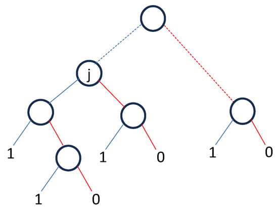
Figure 10.
Generic BDD structure.
On any path through the diagram, the events encountered can be allocated to sets of states of components that feature in one of the dependency groups, or to a set of states of components that fail independently, . The events that are placed in each dependency set will feature the element label and indicate if the path passes through this element on its 1-branch or 0-branch. This combination of events will be labelled Dpath. Similarly, the collection of elements and their state (working or failed) contained in will be labelled Ipath. and are then calculated as follows:
Element j fails independently of all other elements
Noting that on the first term and in the second term calculations, the probability of the events in each Dpath are obtained from the relevant PN or Markov analysis.
Element j belongs to dependency group Dd
5.2. Criticality Measure of Importance
For component i, which fails independently of the other basic events, the calculation of the criticality measure remains, as specified in Equation (5), and can be accomplished cheaply having obtained Birnbaum’s measure of importance.
For basic events that belong to one of the dependency groups, the criticality function and the component failure probability cannot be multiplied together, and the probability that the module is in a critical state and the basic event has failed needs to be evaluated when considering the analysis of the relevant Petri net or Markov model for the dependency. The criticality measure of importance is given as follows:
where is the probability that the dependent module that contains i is critical for event i and i failure.
5.2.1. Dependent Component Failures in a Markov Model
When calculating the criticality measure of importance for a component that features in a Markov dependency model, Equation (25) is used. It is required to calculate the term from the Markov model. As when calculating Birnbaum’s measure, it is necessary to consider the definitions of the states represented on the Markov State Transition Diagram. It is required to identify those states where the system was in a critical state for component i and then component i fails, leading to system failure. The probability of these states are then summed to calculate .
As an example, consider the calculation of for the Markov model illustrated in Figure 9a. The critical state for component A is State 4. As is shown in the diagram, when A fails from State 4, the system transitions to State 5 and the system fails, as follows:
For the Markov model illustrated in Figure 9b, the critical state for component A is State 1, and the failure of component A advances to system failed state 2, as follows:
5.2.2. Dependent Component Failures in a Petri Net Model
The approach taken to calculate the criticality measure of importance for a component included in a Petri net module follows that used to calculate Birnbaum’s measure of importance for Petri net models where the times of residing in certain condition states are logged during the simulation. For all component failures that appear in a dependency group, the criticality importance measure is then calculated using Equation (25), where the analysis of the Petri net will deliver the term in the equation.
To calculate , it is necessary to monitor the simulation time in the following states:
The system has failed and component i has failed: .
The system has failed and component i is working: .
Total simulation time: .
5.3. Risk Achievement Worth and Risk Reduction Worth Measures
The expression used to calculate Risk Achievement Worth is given in Equation (6). All the terms of this equation have been previously considered during the system assessment and the evaluation of during the quantification of Birnbaum’s measure of importance. Therefore, this importance measure can be calculated very cheaply.
The same is true for Risk Reduction Worth, which requires , which is again evaluated during the production of Birnbaum’s measure of importance, along with , to quantify Equation (7).
6. Case Study: Pressure Cooling Vessel System
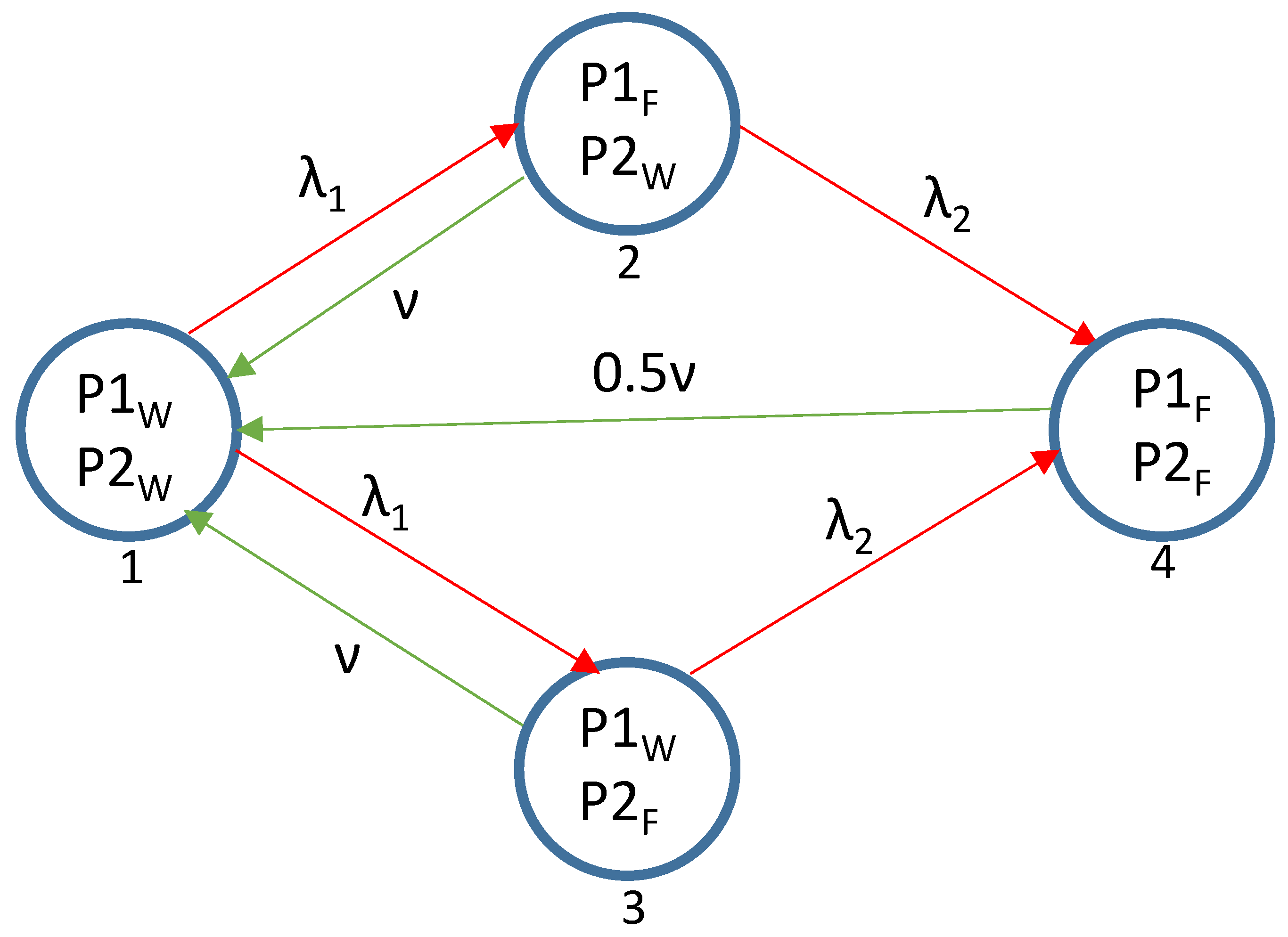
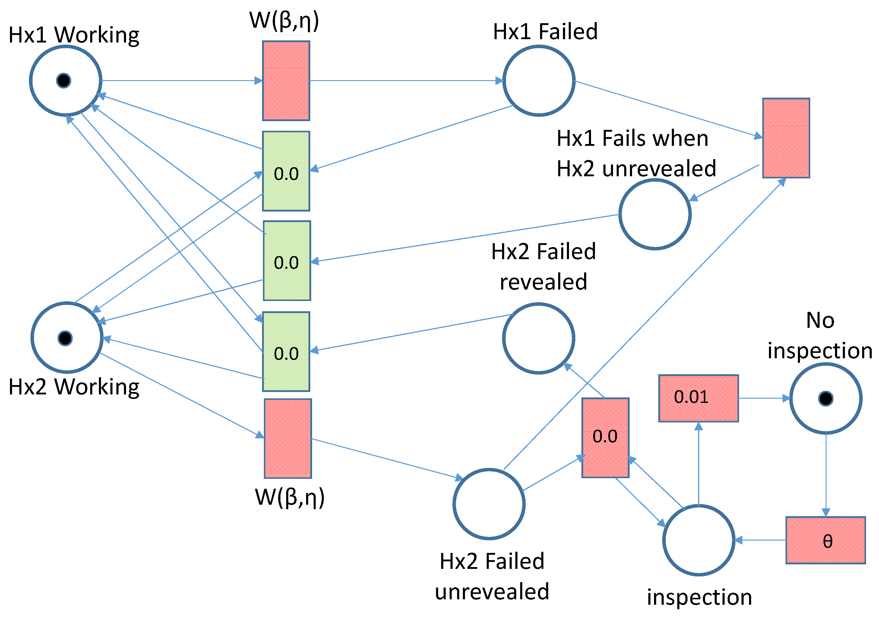
To illustrate the approach used to calculate each of the importance measures, consider the pressure cooling vessel system introduced in Section 2. The dependencies between P1 and P2 are modelled in the Markov diagram shown in Figure 11. Figure 12 contains the Petri net used to model the relationship between the heat exchangers Hx1 and Hx2.
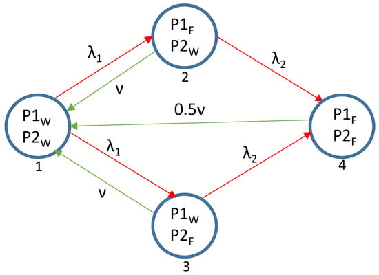
Figure 11.
Markov model for secondary failure dependency.
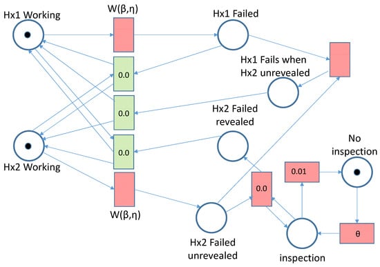
Figure 12.
Petri net model for opportunistic maintenance.
The analysis of the fault tree using the D2T2 algorithm to obtain the top event failure probability () will, as intermediate stages, calculate the probability of all of the complex factors, the probability of dependent events Hx1 and Hx2 with a Petri net evaluation and the probability of the P1- and P2-dependent events through the use of Markov assessment. These will then be substituted into the BDD calculations to predict top event performance. All of these calculations are retained for use in evaluating the component importance measures.
A comprehensive assessment of the importance measures for all components in the pressure cooling vessel system is given stage by stage in the following sections.
6.1. Birnbaum’s Measures of Importance
The criticality function is evaluated for each of the independent modules identified in the D2T2 modularisation process. These are considered in the following sections, first considering the independent complex factors, Cf2–Cf6; Cf1 represents the dependent event combination P1.P2 and will be considered later.
6.1.1. Criticality Function Terms for Independent Complex Factors
The criticality function for Cf2 = S1.S2 is given in Table 4. The terms in the table are obtained using Equations (15) and (16) for complex factors with an AND operator.

Table 4.
The criticality function of Cf2 with respect to its input factors.
Table 5 contains the criticality function for the complex factor Cf3 = Comp + R1 + Fan + Motor + R2 + T2 + V1 with respect to its inputs. The factor has seven basic events as inputs to an OR operator, and the terms are, therefore, evaluated using Equations (11) and (12).

Table 5.
The criticality function of Cf3 with respect to its input factors.
Complex factor 4, Cf4 = P3, is a simple combination of the failure modes for pump P3, and since it only has one input, its criticality function evaluation is trivial, as shown in Table 6.

Table 6.
The criticality function of Cf4 with respect to its single input.
The final two complex factors are both OR combinations of events. Cf5 = Cf1 + T1, combines a complex factor and a basic event as inputs, whereas the inputs to Cf6 = Cf2 + Cf3 + Cf4 are all complex factors. The criticality function evaluations of Cf5 and Cf6 are given in Table 7 and Table 8, respectively. As with Cf3, Equations (11) and (12) are utilised.

Table 7.
The criticality function of Cf5 with respect to its inputs.

Table 8.
The criticality function of Cf6 with respect to its inputs.
6.1.2. Criticality Function Terms for Dependent Complex Factors
Complex factor Cf1 = P1.P2 represents the AND combination of dependent events P1 and P2, which are modelled through the use of the Markov model to deliver both their combined probability and the probability of the individual event combinations. The terms needed to calculate the criticality function for this factor are shown in Table 9 and taken from the results of the Markov model analysis.

Table 9.
The criticality function of Cf1 with respect to its dependent inputs.
6.1.3. Criticality Function Terms for BDDs
Two BDDs, shown in Figure 7, are utilised in the D2T2 analysis of the fault tree. The first represents the top event, Sys, it has two inputs, gate G1 and basic event PoW. These inputs are independent, and the terms in the criticality function evaluation, given in Table 10, are obtained using Equations (21)–(23).

Table 10.
The criticality function of the top event BDD with respect to its inputs.
The second BDD represents the causes of gate G1 in the original fault tree and has four inputs: independent complex factors Cf5 and Cf6, along with dependent basic events Hx1 and Hx2.
For the criticality of G1 with respect to Cf5, Cf5 is a component in a dependency BDD, , and so Equations (21), (22) and (24) are applied considering dependency group, D2 = {Hx1, Hx2}. There are four paths through the BDD (Shown in Figure 7), as follows:
Cf51 . Cf61
Cf51 . Cf60 . Hx21
Cf50 . Hx11 . Cf61
Cf50 . Hx11 . Cf60 . Hx21
These give the following:
where , and are obtained from the original analysis of the Petri net, as shown in Figure 12.
6.1.4. Component Criticality Function Evaluations
The results presented in Table 4, Table 5, Table 6, Table 7, Table 8, Table 9, Table 10 and Table 11 show the criticality function for each of the independent modules of the original fault tree with respect to their inputs. These are the basic building blocks used to evaluate Birnbaum’s Measure of importance (criticality function) for each basic event. Table 12 shows the expression used to evaluate each component’s importance measure and, in the third column, the evaluation of this expression. The expression to give each measure of component importance is obtained from the structure of the modules in evaluating t system performance, given in Figure 8.

Table 11.
The criticality function of the gate G1 event BDD with respect to its dependent inputs.

Table 12.
The component criticality functions (Birnbaum’s Measure of Importance).
As an example, consider basic event S1, the case of temperature sensor failure. S1 fails independently of other basic events in the fault tree.
Using the model structure diagram shown in Figure 8, the influence of S1 on the top event comes through as follows:
Using Equation (8) gives the following expression for the criticality function of S1:
The first term of this expression, , is given in Table 10, which relates the criticality function of SYS in terms of its inputs that includes G1.
The criticality function of G1 with respect to its input Cf6 is given in Table 11 as follows:
Substituting terms 31–34 into Equation (30) gives the following:
where dependent basic events are involved in evaluating their criticality function, which will require probabilities calculated from the relevant Markov model or Petri Net that represent their dependencies.
When considering the complex event represented by Cf1 = P1.P2 is represented by the Markov model shown in Figure 11, and thus, the discussion in Section 5.1.2 is relevant. The states in the Markov model with component P1 failed are labelled 2 and 4. Of these, only state 4 results in system failure. Therefore, . Since there are no states when component P1 is working that result in system failure , and:
For the heat exchanger, Hx1 is in Dependency Group 2, along with the second heat exchanger, Hx2. The dependency between the heat exchangers is accommodated in the Petri net model, which feeds into the dependency BDD that represents the gate event G1. The criticality function is then as follows:
is obtained by evaluating and from the G1 BDD:
Giving:
where is obtained from the Petri net model solution.
6.2. Criticality Measures of Importance
Having calculated Birnbaum’s measure of importance (the criticality function), , for those components that fail independently, it is a simple step to evaluate the criticality measure of importance using Equation (5) since Birnbaum’s measure of importance and the probability of component failure are independent.
Of the components in the pressure vessel cooling system, P1, P2, Hx1 and Hx2 belong to dependency groups. In this case, the criticality function, , and the component failure probability will be dependent. P1 is dependent upon P2, and this dependency is modelled using the Markov model shown in Figure 11. Hx1 and Hx2 are dependent events modelled with the Petri net shown in Figure 12.
The calculation process that considers dependent events for the criticality measure is described in Section 5.2.1 and Section 5.2.2.
The criticality measure calculations for P1 and Hx1 are explained below.
P1(Pump1 fails)
The route from P1 to the fault tree top event passes through the following modules:
Using Equation (25), the criticality measure of importance is as follows:
where is the probability that the system is in a critical state for component P1 and P1 has failed, leading to system failure. From the Markov model for this section of the problem shown in Figure 11, it can be seen that .
Hx1 (Heat Exchanger 1 fails)
The heat exchanger’s criticality measure of importance is given as follows:
where is the probability that the system has failed and component Hx1 has failed, leading to system failure. This probability is logged during the simulation of the Petri net shown in Figure 12 and substituted into Equation (40).
6.3. RAW and RRW Measures of Importance
To calculate the values of and the values for and are required along with resulting from the D2T2 analysis system assessment.
To calculate the RAW measure of component importance using Equation (6), is required. This is evaluated using the results of each of the independent modules (complex factors, BDDs, Markov models and Petri nets) derived when calculating . The basic event probability is set to 1, and this is then propagated up through the hierarchical analysis module structure (shown in Figure 8) to re-process the top event to produce system failure probability. The relevant equations used for the modules influenced by each of the basic events are shown in the second column of Table 13. Combining these equations gives in the third column of the table.

Table 13.
The probability of system failure dependent upon each component failure.
The RRW measure of component importance is given in Equation (7) and requires the evaluation of . This is processed by substituting the basic event failure probability of 0 and re-calculating the system failure probability. The results of this process are reported in Table 14. For practical system evaluations, the results for and can be calculated as shown in Table 12 and Table 13 and then by taking their difference, as shown in Equation (2).

Table 14.
The probability of system failure dependent upon each component functioning.
7. Conclusions
This paper shows how the Birnbaum, Criticality, Risk Assessment Worth and Risk Reduction Worth component importance measures can be calculated when system failure modelling has been accomplished using a fault tree evaluated using the D2T2 methodology. The calculation process can be implemented very efficiently as the majority of the computational effort goes into evaluating Birnbaum’s Measure of Importance, also known as the criticality function, . This takes advantage of the efficient hierarchical structure of independent modules created by the D2T2 framework. The criticality functions of each of the independent modules, with respect to their input variables, are obtained, and the calculation of becomes the product of the relevant module criticality functions.
Once has been evaluated, there is relatively little computational effort required to calculate the criticality measure of importance rankings, .
For the Risk Assessment Worth, and Risk Reduction Worth, additional calculations have to be performed to calculate . Again, this can be carried out efficiently by re-using the intermediate module probabilities calculated during the original execution of the D2T2 methodology to deliver the top event probability and frequency. is obtained by repeating the top event quantification conditional on each component having failed. is then used directly to produce the Risk Assessment Worth.
Subtracting from gives a rapid calculation of , which enables the Risk Reduction Worth measure to be calculated.
Incorporating the calculation of importance measures into the D2T2 methodology extends the current analysis capabilities in terms of providing quantifiable measures that can be interpreted to identify the weaknesses in the system. Changes can then be implemented that improve system performance. For this implementation, the system assessed can feature dependencies between the components, complex maintenance processes and components with any distributions of times to failure or repair. From a practical point of view, this new advance enables system performance to be improved, making systems safer by using the available resources in the most effective way.
Author Contributions
Conceptualization, J.A. and S.L.; Methodology, J.A. and S.L.; Supervision, J.A.; Project administration, J.A. All authors have read and agreed to the published version of the manuscript.
Funding
This work was supported by the Lloyd’s Register Foundation (GA\100170), a charitable foundation in the U.K. helping to protect life and property by supporting engineering-related education, public engagement, and the application of research.
Data Availability Statement
Data are contained within the article.
Conflicts of Interest
The authors declare no conflict of interest.
References
- Apostolakis, G. How Useful is Quantitative Risk Assessment? Risk Anal. 2004, 24, 515–520. [Google Scholar] [CrossRef] [PubMed]
- Vesely, W.E. A Time Dependent Methodology for Fault Tree Evaluation. Nucl. Eng. Des. 1970, 13, 337–360. [Google Scholar] [CrossRef]
- Andrews, J.D.; Moss, T.R. Reliability and Risk Assessment, 2nd ed.; Professional Engineering Publishing: London, UK, 2002; 540p, ISBN 1-86058-290-7. [Google Scholar]
- Zhang, Q.; Mei, Q. Element Importance and System failure frequency of a 2-State System. IEEE Trans. Reliab. 1985, 34, 308–313. [Google Scholar] [CrossRef]
- Dunglinson, C.; Lambert, L. Interval Reliability for Initiating and Enabling Events. IEEE Trans. Reliab. 1983, 32, 150–163. [Google Scholar] [CrossRef]
- Rauzy, A. Toward an Efficient Implementation of the MOCUS Algorithm. IEEE Trans. Reliab. 2003, 52, 175–180. [Google Scholar] [CrossRef]
- Čepin, M. Analysis of truncation limit in probabilistic safety assessment. Reliab. Eng. Syst. Saf. 2005, 87, 395–403. [Google Scholar] [CrossRef]
- Rauzy, A. New algorithms for Fault Trees Analysis. Reliab. Eng. Syst. Saf. 1993, 59, 203–211. [Google Scholar] [CrossRef]
- Sinnamon, R.M.; Andrews, J.D. Quantitative Fault Tree Analysis Using Binary Decision Diagrams. Eur. J. Autom. 1996, 30, 1051–1071. [Google Scholar]
- Sinnamon, R.M.; Andrews, J.D. Improved Accuracy in Quantitative Fault Tree Analysis. Qual. Reliab. Eng. Int. 1997, 13, 285–292. [Google Scholar] [CrossRef]
- Sinnamon, R.M.; Andrews, J.D. Improved Efficiency in Qualitative Fault Tree Analysis. Qual. Reliab. Eng. Int. 1997, 13, 293–298. [Google Scholar] [CrossRef]
- Bouissou, M.; Bruyere, F.; Rauzy, A. BDD Based Fault Tree Processing: A Comparison of Variable Ordering Heuristics. In Proceedings of the European Safety and Reliability Association Conference, ESREL’97, Lisbon, Portugal, 17–20 June 1997; Volume 3, pp. 2045–2052. [Google Scholar]
- Bartlett, L.M.; Andrews, J.D. Choosing a Heuristic for the Fault Tree to Binary Decision Diagram Conversion, using Neural Networks. IEEE Trans. Reliab. 2002, 51, 344–349. [Google Scholar] [CrossRef]
- Xing, L.; Amari, S.V. Binary Decision Diagrams and Extensions for System Reliability Analysis; Wiley: Hoboken, NJ, USA, 2015; ISBN 978-1-118-54937-7. [Google Scholar]
- Farahani, A.; Shoja, A.; Tohidi, H. Chapter 6—Markov and Semi-Markov Models in System Reliability. In Advances in Reliability Science; Garg, H., Ram, M., Eds.; Engineering Reliability and Risk Assessment; Elsevier: Amsterdam, The Netherlands, 2023; pp. 91–130. ISBN 9780323919432. [Google Scholar]
- Ould El Medhi, S.; Leclercq, E.; Lefebvre, D. Identification of Stochastic and deterministic Petri Net Models for Reliability Analysis. Proc. Inst. Mech. Eng. Part O J. Risk Reliab. 2008, 223, 13–26. [Google Scholar] [CrossRef]
- Li, R.; Reveliotis, S. Performance Optimization for a Class of Generalized Stochastic Petri Nets. Discret. Event Dyn. Syst. 2015, 25, 387–417. [Google Scholar] [CrossRef][Green Version]
- Meshkat, L.; Dugan, J.B.; Andrews, J.D. Dependability Analysis of Systems with On-demand and Active Failure Modes, Using Dynamic Fault Trees. IEEE Trans. Reliab. 2002, 51, 240–251. [Google Scholar] [CrossRef]
- Zhou, S.; Ye, L.; Xiong, S.; Xiang, J. Reliability Analysis of Dynamic Fault Trees with Priority-AND Gates Based on Irrelevance Coverage Model. Reliab. Eng. Syst. Saf. 2022, 224, 108553. [Google Scholar] [CrossRef]
- Andrews, J.D.; Tolo, S. Dynamic and Dependent Tree Theory (D2T2): A Framework for the Analysis of Fault Trees with Dependent Basic Events. Reliab. Eng. Syst. Saf. 2023, 230, 108959. [Google Scholar] [CrossRef]
- Birnbaum, Z.W. On the importance of different component in a multi-component system. In Multivariate Analysis II; Krishnaiah, P.R., Ed.; Academic Press: Cambridge, MA, USA, 1969. [Google Scholar]
- Amrutkar, K.P.; Kamalja, K.K. An overview of various importance measures of reliability system. Int. J. Math. Eng. Manag. Sci. 2017, 2, 150–171. [Google Scholar] [CrossRef]
- Rausand, M.; Hoyland, A. System Reliability Theory, Models, Statistical Methods and Applications, 2nd ed.; Wiley: Hoboken, NJ, USA, 2004. [Google Scholar]
- Platz, O.; Olsen, J.V. FAUNET: A Program Package for Evaluation of Fault Trees and Networks; Report No 348; Research Establishment Riso: Roskilde, Denmark, 1976. [Google Scholar]
- Reay, K.; Andrews, J.D. A Fault Tree Analysis Strategy Using Binary Decision Diagrams. Reliab. Eng. Syst. Saf. 2002, 78, 45–56. [Google Scholar] [CrossRef]
- Dutuit, Y.; Rauzy, A. A Linear-Time Algorithm to find Modules of Fault Trees. IEEE Trans. Reliab. 1996, 45, 422–425. [Google Scholar] [CrossRef]
- Van der Borst, M.; Schoonakker, H. An Overview of PSA Importance Measures. Reliab. Eng. Syst. Saf. 2001, 72, 241–245. [Google Scholar] [CrossRef]
Disclaimer/Publisher’s Note: The statements, opinions and data contained in all publications are solely those of the individual author(s) and contributor(s) and not of MDPI and/or the editor(s). MDPI and/or the editor(s) disclaim responsibility for any injury to people or property resulting from any ideas, methods, instructions or products referred to in the content. |
© 2024 by the authors. Licensee MDPI, Basel, Switzerland. This article is an open access article distributed under the terms and conditions of the Creative Commons Attribution (CC BY) license (https://creativecommons.org/licenses/by/4.0/).

