Stochastic Orderings of the Idle Time of Inactive Standby Systems

Abstract

In this paper, we consider a failed cold standby system and obtain stochastic bounds on the idle time of such systems. We state and prove that if the last spare in the system is exponentially distributed and if the components have log-concave lifetime distributions, then the idle time of a failed cold standby system is smaller than the sum of the idle times of the components in the system according to the likelihood ratio order. In order to compare the idle time of two cold standby systems with different numbers of spares and different observation times of the failure in terms of the likelihood ratio order, an additional result is presented. Finally, we establish sufficient conditions for the usual stochastic ordering between the idle time of a cold standby system of size two and the sum of the idle times of the components in the system. We provide several examples to show that the results are achievable.

1. Introduction

Consider n components operating sequentially with random lifetimes $X_1,X_2,\cdots ,X_n$ such that the first component starts operating at time $\tau =0$ and has random lifetime $X_1$ while the remaining $(n-1)$ components do not operate and remain in standby mode. At time $\tau =X_1$, when the first component fails, the second component immediately starts working and has a random lifetime $X_2$; at time $\tau =X_1+X_2$, when the second component fails, the third component immediately starts working, etc., such that at time $\tau =X_1+X_2+\cdots +X_n$ the system fails. This is called a cold standby system with n units, in which the components work one after another until then the last component fails. Suppose that at the time $\tau =t$, when an operator has performed an inspection, it is determined that the cold standby system is inactive. The idle time of the cold standby system is a dynamic random variable of the system that depends on the time t at which the system was found to be inactive. Thus, it is assumed that an interval of time has elapsed since the system was found to be inactive, implying that the observation of the system’s failure was lagged. It is assumed that $X_1,X_2,\cdots ,X_n$ are independent; however, in general, they may not be identically distributed, for instance, if different types of components are installed in the system.

Single- and dual-unit redundant systems have been the subject of extensive research in the reliability literature because of their widespread use in modern business and industrial systems. Parallel and standby redundancy are the two main forms. In a standby system, the redundant units are not included in the system from the beginning, and are only included when they are needed, whereas in a parallel system they are included from the beginning. There are three types of standby units: cold, warm, and hot. Cold standby sparing is a reliable way to ensure that a system can continue to function as intended even if some of its components fail. In this technique, redundant standby elements are kept in a powerless cold mode to conserve resources and protect them from workloads. If an online component fails, a cold standby component can be activated to take over. Because a cold standby unit is unplugged and completely inactive, it cannot fail until the primary unit is replaced. Because it is only partially energized, a warm standby unit has a lower load. Although redundant, a hot standby device is fully functional in the system. The lifespan of cold standby systems can be described as being longer than other types of backup systems because they are not actively operated and as such are subject to less wear and tear. This can result in cost savings for organizations, as they do not need to replace or upgrade the system as frequently. However, the life of the system can be affected by factors such as the quality of the hardware and software used, maintenance practices, and frequency of use. Cold standby systems are commonly used in reliability to support critical systems and processes. Example applications of cold standby systems in reliability include:

(1) Data backup and recovery: cold standby systems can be used to store backup data and ensure its availability in the event of a system failure or malfunction.

(2) Emergency power supply: cold standby systems can be used as a backup power supply in the event of a power failure or malfunction to ensure that critical systems remain operational.

(3) Network redundancy: cold standby systems can be used for network redundancy to ensure that critical network services remain available in the event of a network outage or failure.

(4) Server redundancy: cold standby systems can be used for server redundancy to ensure that critical applications and services remain available in the event of a server failure or defect.

(5) Disaster recovery: cold standby systems can be used as part of a disaster recovery plan to provide backup support for critical systems and processes in the event of a natural disaster or other catastrophic event.

Overall, cold standby systems are an important tool for ensuring the reliability and availability of critical systems and processes. They can help organizations to minimize downtime and maintain continuity in the face of unexpected events. For example, k-out-of-n systems are a type of reliability system in which a system is considered functional as long as k or more of n components are functioning properly; in other words, the system fails only when fewer than k components are functioning properly. This type of system is often used in engineering and manufacturing applications where redundancy is required to ensure the system’s continued functionality even if some of its components fail. The values of k and n can vary depending on the specific application and the level of reliability required. A situation in which such a standby system is used is that of k-out-of-n systems (see, e.g., Levitin et al. [1], Fernández [2], Barron and Yechiali [3], Barron [4], Levitin et al. [5], Bian et al. [6], and references therein). The method of cold standby has been widely utilized in crucial scenarios such as flight controls, satellites, chemical process controls, telecommunication systems, and nuclear power plants (see, for instance, Mathur [7], Wang [8], Johnson and Julich [9], Sinaki [10], Pandey et al. [11], Coit [12], Hsieh and Hsieh [13], Elerath and Pecht [14], and Wang et al. [15]).

Cold standby systems have recently attracted the attention of many researchers in the field of reliability enginerring (see, e.g., Wang and Ye [16], Ramezani Dobani et al. [17], Danjuma et al. [18], Malhotra et al. [19], and Lin et al. [20]).

In contrast to the residual life of a system, one aspect of engineering systems is their idle time. The idle time is sometimes called the inactivity time or reversed residual lifetime. In view of the idle time, the stochastic properties of coherent systems, a large and well-known class of systems in reliability, have been widely studied during the past decades (see, for instance, Bayramoglu and Ozkut [21], Zhang and Balakrishnan [22], Navarro et al. [23], Kayid et al. [24], Navarro and Calì [25], Salehi and Tavangar [26], Toomaj and Di Crescenzo [27], Amini-Seresht et al. [28], Guo et al. [29], and Kayid and Shrahili [30]). However, the study of stochastic comparisons between idle (or inactive) time of cold standby systems has not been conducted in literature to date.

In this paper, we present results on a failed cold standby system. Two scenarios using different strategies are compared based on their idle time. The first scenario assumes that a cold standby system with n units (with the first unit being the underlying component in the system and the remaining $(n-1)$ components the spare components) has failed before a time t at which the operator found the system to be in failure state, resulting in an idle time on the part of the cold standby system. In the second scenario, we assume that n components were used separately in n independent experiments, in which all components failed before t and the idle time of all components was measured at time t; we then consider the sum of the idle times of the n components. The goal of this work is to derive lower and upper bounds for the idle time of the cold standby system with n components with heterogeneous lifetime distributions by using the sum of the idle time of these n components separately.

The remainder of the paper is divided as follows. Section 2 discusses related research in the relevant fields. In Section 3, preliminary notion and basic formulas and definitions are provided. Section 4 presents the main results of the paper. In Section 5, we conclude the paper with a summary of our results and findings along with further directions for possible future studies.

2. Further Descriptions and Related Works

The concept of stochastic comparisons of the residual life of the convolution of random variables has attracted the attention of many researchers in the context of reliability theory and risk analysis. Thus, Ahmed and Kayid [31] considered the residual lifetime of convolutions of random lifetimes and derived sufficient conditions under which convolution residuals are preserved under the Laplace transform order. Amiripour et al. [32] used folding residuals based on observations from one or two samples to construct a set of stochastic orderings. In this way, they found computable constraints on both the predicted values of the convolution residuals and the survival functions. In addition, their work discussed applications in queueing theory and reliability theory. In the same direction, Kayid and Alshehri [33] recently developed stochastic comparisons between the lifetime of a used cold standby system with a certain age t (which is still working) and the sum of the remaining lifetimes of the components in the system. They used the usual stochastic order and likelihood ratio order to derive their main results. They obtained a result and presented sufficient conditions under which a used cold standby system is less reliable in terms of likelihood ratio order than a cold standby system with used components when the used components have a common age t.

In the context of reversed residual lifetime or inactivity time of the convolution of random variables, the stochastic comparisons obtained in the literature are based on mean inactivity time functions. For example, Ahmad et al. [34] derived a preservation property of the mean inactivity time order under the convolution of random lifetimes. Ortega [35] presented findings that provide guidelines for the total loss amounts for two insurance portfolios under the collective risk model (random sums). In this way, it is possible to analyze the idle time of a cold standby system using the mean values according to the results of Ahmad et al. [34] and Ortega [35]. However, there is a research gap in this area in that there have been no studies analyzing the idle time of cold standby systems using more general distribution measures such as the distribution of inactivity time; thus, there is much room for further research in this area.

In the present paper we consider the idle time of a failed cold standby system to obtain lower and upper bounds for it in terms of the idle time of the failed components in the system. As pointed out and clearly shown by Ahmad et al. [34], the results for the idle variable (the inactivity time) cannot be concluded from the similar results on the residual lifetime variable. Thus, there is room to fill another gap in the literature, which is the starting point for our study in this paper. Another focus is that the properties we obtain in this paper are quite different from and cannot be acquired using the results in Kayid and Alshehri [33]. An interesting point is that, in general, in the remaining lifetime of a functioning coherent system. This is because the idle variable takes values at $[0,t)$, while the residual lifetime variable takes values at $(t,+\infty )$; thus, the former is obviously more predictable than the latter. Therefore, the problem of finding the stochastic bounds of the idle time of a cold standby system has a complementary role in refining our knowledge about the lifetime of the system.

It is worth mentioning that the results obtained in this work play a complementary role compared to the previous works in this field (i.e., Kayid and Alshehri [33]). In that work, the authors were concerned with the remaining lifetime of cold standby systems. In contrast, in the current study we focus on the inactivity time of cold standby systems and the comparison of systems from the point of view of the idle time. The results obtained in this work can be useful in practice for several purposes. The observation time at which a cold standby system is classified as inactive may not correspond exactly to the time at which it actually failed. As a result, there is a time interval during which the system is inactive, which can lead to further costs and losses. Therefore, it is important to control the situation and use an appropriate number of components in the system or even components with a certain reliability level to minimize the idle time of the cold standby system. In this direction, the results of this paper can provide further guidance for engineers to design suitable structures for cold standby systems. The assumptions made in this paper include aging properties of the lifetime distributions of the components of the system along with ordering properties and relationships with the lifetime distributions of the components. Because equipping any system or its components with standby spare parts is a relevant method to increase the reliability of systems with different structures, in the case where a cold standby system with two units or components is considered, the results of this paper may be useful to maintain other kinds of systems to ensure that the main unit is considered as a system with any structure (i.e., not exactly a cold standby system) or a component within it.

The problem of finding stochastic upper and lower bounds for the distribution of convolution of random variables ($S_n={\sum }_{i=1}^n{X}_i$, see Section 3 for further descriptions), and more generally the mathematical expectations of functions of $S_n$, is of particular interest in the context of risk theory and actuarial analysis. This is particularly useful; it is not plain to derive the distribution function of the convolution of random variables, as they ordinarily have no closed tractable forms. As mentioned by Ramsay [36], while the Pareto distribution is an important candidate for actuaries and economists, an exact expression for the distribution of the sum of n i.i.d. (independent and identically distributed) Pareto random variables is generally difficult to obtain. In the actuarial literature, there is increasing worry about the impact of dependence between individual risks $X_1,\cdots ,X_n$ on the distribution of the total claim $S_n$. Research by Dhaene et al. [37] has resulted in, among other things, the identification of the portfolio producing the smallest and largest stop-loss premiums, resulting in bounds on $E\left(S_n\right)$ for any arbitrary non-decreasing and convex functions in circumstances of dependence between the $X_i$s. In order to further these findings, Denuit et al. [38] demonstrated how to calculate constraints on $P(S_n>s)$, and more broadly on $E\left(S_n\right)$, for monotone functions that are not always convex.

There has been an increasing interest in evaluating claims and risks in the context of conditional distributions. In risk analysis, the conditional tail expectation is an important metric for right-tailed risk. It indicates the expected level of risk that may occur when an expected risk exceeds a threshold t. Cai and Li [39] studied the convolution and extreme values of dependent risks that follow a multivariate phase type distribution; they derived explicit formulas for a set of conditional tail expectations of the convolution and extreme values for such dependent risks. Their method provided structural information about these distributions while providing novel distributional properties for multivariate phase-type distributions by exploiting the underlying Markovian property of these distributions. In another work by Sordo et al. [40], they studied the marginal behavior of the i-th risk in a risk portfolio in the presence of adversity, such as a disproportionate loss to the portfolio or, in the case of a portfolio with a positive dependence structure, a disproportionate loss to another risk. They formalized the notion that the i-th component of the portfolio is riskier when it is part of a positive-dependent random vector than when it is considered alone, which they did in several ways by considering specific conditional risk distributions. In addition, they acquired conditions under which, given two random vectors with a defined dependence structure, the existence of specific stochastic orderings between their marginals implies an ordering between the corresponding conditional risk distributions.

3. Preliminaries

In the remaining parts of the paper, we use the following notation. Let $X̠=(X_1,\dots ,X_n)$ be a random vector, denote $S_n={\sum }_{i=1}^n{X}_i$, and consider a cold standby system comprising n components. First, one component begins to work and the residual $n-1$ components are in standby and ready to lie in the system. Upon the failure of the first component, the components that are in queue in standby mode are replaced one by one until all components become inactive and the cold standby system fails. Suppose that $X_1,\dots ,X_n$ represent the lifetimes of n described components having cumulative distribution functions (CDFs) $F_{X_1},\dots ,F_{X_n}$. It is assumed that $X_1,\dots ,X_n$ are independent. The lifetime of the cold standby system is then identified as

$$S_n=X_1+X_2+\dots +X_n.$$

(1)

Although in this paper we use the random variable (rv) $S_n$ in (1) as the lifetime of an n-fold cold standby system, there is another description for this rv from the perspective of insurance and risk theory. In such frameworks, convolution manifests itself naturally. In this case, the portfolio consists of a fixed number of different insurance policies and the total loss of the portfolio is the sum (convolution) of the random losses of the individual policies, which is consistent with the model of individual risk. For example, we are interested in how the sum $S_n$ of claims is distributed across different insurance policies, where $X_i,i=1,2,\dots ,n$ represents the payout on policy i. It is assumed that the risks $X_i$ are independent random variables. The risks should be combined into one term in (1) if this assumption is broken for certain risks, such as fire insurance policies for different floors of the same building. The CDF of the lifetime of the cold standby system is

$$F_{S_n}\left(t\right)=P(X_1+X_2+\dots +X_n\le t)=F_{X_1}\left(t\right)\ast F_{X_2}\left(t\right)\ast \dots \ast F_{X_n}\left(t\right),$$

(2)

in which ∗ stands for the convolution operator. It is acknowledged that when $X_i$ and $X_j$, for $i\ne j$ are independent, then $F_{X_i}\left(t\right)\ast F_{X_j}\left(t\right)={\int }_{-\infty }^{+\infty }{F}_{X_i}(t-x)f_{X_j}\left(x\right)dx,$ where $f_{X_j}$ is the probability density function (PDF) of $X_j$, which is the CDF of the convolution of $X_i$ and $X_j$, that is, the CDF of $X_i+X_j$. From (2), we can develop the following:

$$F_{S_n}\left(t\right)=F_{S_{n-1}}\left(t\right)\ast F_{X_n}\left(t\right)={\int }_{-\infty }^{+\infty }{F}_{S_{n-1}}(t-x)f_{X_n}\left(x\right)dx.$$

(3)

Suppose that X denotes the life length of a lifetime organism. We assume that at the time t at which an inspection is carried out, it is found that the organism is not alive or the system is not working. This situation is frequently encountered in different contexts; there is no process to accurately determine the time point at which the organism failed, though there may be signs from which can be realized that the organism has failed. There are many situations in which the observation of events is postponed. Thus; the time t may be the first time at which a sign has observed. We utilize the rv $X_{\left(t\right)}=(t-X|X\le t)$, which is well-defined for every $t\ge 0$ for which $F_X\left(t\right)>0$. The rv $X_{\left(t\right)}$ is called the inactivity time of the organism (which has a random lifetime X) at time t. The rv $X_{\left(t\right)}$ has the following CDF.

$$F_{X_{\left(t\right)}}\left(x\right)=\left\{\begin{array}{cc}0,\hfill & \hfill x<0\\ 1-\frac{F_X(t-x)}{F_X\left(t\right)},\hfill & \hfill 0\le x<t\\ 1,\hfill & \hfill x\ge t\end{array}\right.$$

(4)

The associated reliability function of $X_{\left(t\right)}$ is obviously

$${\overline{F}}_{X_{\left(t\right)}}\left(x\right)=\left\{\begin{array}{cc}1,\hfill & \hfill x<0\\ \frac{F_X(t-x)}{F_X\left(t\right)},\hfill & \hfill 0\le x<t\\ 0,\hfill & \hfill x\ge t\end{array}\right.$$

(5)

and the PDF of $X_{\left(t\right)}$ is derived by taking derivation of Equation (4), as shown below.

$$f_{X_{\left(t\right)}}\left(x\right)=\left\{\begin{array}{cc}\frac{f_X(t-x)}{F_X\left(t\right)}\hfill & \hfill :0\le x<t\\ 0\hfill & \hfill :x\ge t\mathrm{or}x<0\end{array}\right.$$

(6)

Note that $F_X\left(t\right)$ is the normalizing constant, as in view of Equation (6) we have $F_X\left(t\right)={\int }_0^t{f}_X(t-x)dx$. There are two well-known reliability measures which are constructed using the rv $X_{\left(t\right)}$, namely, the reversed hazard rate (RHR) function and the mean inactivity (MIT) time function. In view of (6), the RHR of a lifetime rv ($F_X\left(0^{-}\right)=0$) is defined as

$${\tilde{h}}_X\left(t\right)=f_{X_{\left(t\right)}}\left(0\right)=\frac{f_X\left(t\right)}{F_X\left(t\right)},\mathrm{for}\mathrm{all}t:F_X\left(t\right)>0.$$

The MIT function of X, as the mathematical expectation of the rv $X_{\left(t\right)}$, is derived as follows:

$${\tilde{m}}_X\left(t\right)=E\left[X_{\left(t\right)}\right]=\frac{{\int }_0^t{F}_X\left(x\right)dx}{F_X\left(t\right)},\mathrm{for}\mathrm{all}t:F_X\left(t\right)>0.$$

For the preliminary properties of the RHR function, we refer readers to Block et al. [41] and Finkelstein [42]; for the initial aspects and properties of MIT functions, see Kayid and Izadkhah [43] and Khan et al. [44].

Stochastic orders which have been utilized to compare probability distributions provide useful procedures for comparing reliability systems. Two reputable and frequently used stochastic orders are adopted in this paper to construct stochastic orders between the idle times of inactive systems. The following definition is adopted from Shaked and Shanthikumar [45]. Suppose that X and Y have CDFs $F_X$ and $F_Y$, respectively, for which the survival functions (SFs) of X and Y are defined as ${\overline{F}}_X\equiv 1-F_X$ and ${\overline{F}}_Y\equiv 1-F_Y$, respectively.

Definition 1.

Suppose that X and Y are two non-negative rvs with PDFs $f_X$ and $f_Y$ and survival functions ${\overline{F}}_X$ and ${\overline{F}}_Y$, respectively. Then, we say that X is smaller than or equal to Y in:

(i) the likelihood ratio order (denoted as $X{\le }_{lr}Y$) if $\frac{f_Y\left(t\right)}{f_X\left(t\right)}$ is increasing in $t\ge 0$;

(ii) the usual stochastic order (denoted as $X{\le }_{st}Y$) if ${\overline{F}}_X\left(t\right)\le {\overline{F}}_Y\left(t\right)$ for all $t\ge 0$.

The two stochastic orders provided in Definition 1 are in a relation with each other such that $X{\le }_{lr}Y$ yields $X{\le }_{st}Y$ (for an example, see Theorem 1.C.1 in Shaked and Shanthikumar [45]). The usual stochastic ordering is useful for comparing the reliability of two systems directly and completely in the whole time interval. On the other hand, the likelihood ratio ordering is a powerful tool for comparing the strengths of random variables such that $X{\le }_{lr}Y$ holds if and only if

$$\left[X\right|a<X\le b]{\le }_{st}\left[Y\right|a<Y\le b]\mathrm{for}\mathrm{all}a<b,$$

that is, the likelihood ratio order is able to compare two systems with lifetimes X and Y based on their reliability functions at specific times. The likelihood ratio order is useful for constructing rejection regions when testing certain statistical hypotheses in a parametric family of distribution in order to choose between two values of the parameter. For more properties and details on these stochastic orders, we refer readers to Shaked and Shanthikumar [45].

New classes of lifetime distributions can be generated in accordance with the comparison between $X_{\left(t_1\right)}$ and $X_{\left(t_2\right)}$ for all $t_1\le t_2\in {\mathbb{R}}^{+}$ according to the likelihood ratio order and the usual stochastic order. In the sequel to the above-cited paper, the following classes are used.

Definition 2.

The rv X with PDF $f_X$ is said to have the following:

(i) The increasing likelihood ratio property (denoted by $X\in ILR$) whenever $f_X\left(t\right)$ is log-concave in $t\ge 0$;

(ii) A decreasing reversed hazard rate (denoted by $X\in DRHR$) whenever $F_X\left(t\right)$ is log-concave in $t\ge 0$.

For instance, as a standard lifetime distribution, the exponential distribution fulfills both the $ILR$ and $DRHR$ properties. The Weibull distribution with a shape parameter $\alpha$, scale parameter $\lambda$, and reliability function (SF) ${\overline{F}}_X\left(t\right)=exp(-{\left(\lambda t\right)}^{\alpha })$ has the $ILR$ and $DRHR$ properties if $\alpha >1$. For further properties of the $ILR$ and the $DRHR$ classes of lifetime distributions, readers are referred to Lai and Xie [46]. The following definition is from to Karlin [47].

Definition 3.

Let $g(x,y)$ be a non-negative function defined for $x\in \mathfrak{X}\subseteq \mathbb{R}$ and $y\in \mathfrak{Y}\subseteq \mathbb{R}$; then, $g(x,y)$ is said to be totally positive with order 2 (denoted as $T{P}_2$) in $(x,y)\in \mathfrak{X}\times \mathfrak{Y}$ provided that $g(x_1,y_1)g(x_2,y_2)\ge g(x_1,y_2)g(x_2,y_1)$ for all $x_1\le x_2\in \mathfrak{X}$ and for all $y_1\le y_2\in \mathfrak{Y}.$

4. Main Results

Our main results are stated in this section. It is assumed that while the failure of the cold standby system is recognized at time t, the actual time of failure is a time prior to t. The idle time of the inactive cold standby system is measured as the time between the exact time of failure, which is a random variable, and the time t. Here, we use the idle times of the components of the system to obtain lower and upper bounds on the lifetime of the standby system within which they are assembled. Specifically, we show that the idle time of a failed cold standby system with n components at time t is greater than the sum of the idle times of the components in the system minus $(n-1)t$ in the sense of the usual stochastic ordering. The idle time of a cold standby system with n components (one of which active with a random lifetime $X_1$ and the remaining inactive ones $n-1$ with random lifetimes $X_2,\dots ,X_n$ are ready to function upon the failure of the active component) is characterized by the rv:

$${\left(S_n\right)}_{\left(t\right)}:=(t-S_n\mid S_n\le t),\mathrm{for}\mathrm{all}t:F_{S_n}\left(t\right)>0$$

(7)

where t is the time at which the failure of the system is first observed. The results obtained in this paper are derived based on techniques in probability and distribution theory, including the total probability formula.

4.1. Usual Stochastic Order-Based Bounds for the Idle Time of Cold Standby Systems with n Components

In the following theorem we derive a lower bound for the inactivity time of a standby system, in the sense of the usual stochastic order, in terms of the inactivity time of its components.

Theorem 1.

Let $X_1,X_2,\dots ,X_n$ be independent and non-negative rvs such that ${\left(X_1\right)}_{\left(t\right)},{\left(X_2\right)}_{\left(t\right)},\dots ,$ ${\left(X_n\right)}_{\left(t\right)}$ are independent as well; then, for fixed $t\ge 0$,

$${\left(\sum _{i=1}^n{X}_i\right)}_{\left(t\right)}{\ge }_{st}\sum _{i=1}^n{\left(X_i\right)}_{\left(t\right)}-(n-1)t.$$

(8)

Proof. 

We proceed to prove the above theorem using the method of induction. Let $n=2$ and denote $W_n={\left({\sum }_{i=1}^n{X}_i\right)}_{\left(t\right)}$ and $V_n={\sum }_{i=1}^n{\left(X_i\right)}_{\left(t\right)}-(n-1)t$, where $t\ge 0$ is a fixed time. First, we show that ${\overline{F}}_{W_2}\left(a\right)\ge {\overline{F}}_{V_2}\left(a\right)$ for all $a\in \mathbb{R}$. Because for every $n\in \mathbb{N},$$S_{W_n}=[0,t]$ and $S_{V_n}=[-(n-1)t,t]$, we have ${\overline{F}}_{W_2}\left(a\right)\ge {\overline{F}}_{V_2}\left(a\right)$ for all $a\le 0,$ as well as for all $a\ge t$. This is sufficient to show that ${\overline{F}}_{W_2}\left(a\right)\ge {\overline{F}}_{V_2}\left(a\right)$ holds true for all $a\in [0,t]$, which in turn is sufficient to claim that

$$W_2:={(X_1+X_2)}_{\left(t\right)}{\ge }_{st}{\left(X_1\right)}_{\left(t\right)}+{\left(X_2\right)}_{\left(t\right)}-t:=V_2.$$

(9)

For $a\in [0,t]$, we can obtain

$$\begin{array}{cc}\hfill {\overline{F}}_{W_2}\left(a\right)& =\frac{F_{X_1+X_2}(t-a)}{F_{X_1+X_2}\left(t\right)}\hfill \\ \hfill & =\frac{{\int }_0^{t-a}{F}_{X_2}(t-a-x_1)f_{X_1}\left(x_1\right)d{x}_1}{{\int }_0^t{F}_{X_2}(t-x_1)f_{X_1}\left(x_1\right)d{x}_1}\hfill \\ \hfill & =\frac{{\int }_a^t{F}_{X_2}(x-a)f_{X_1}(t-x)dx}{{\int }_0^t{F}_{X_2}\left(x\right)f_{X_1}(t-x)dx},\hfill \end{array}$$

where the first identity follows from Equation (4), the second is obtained using the total probability formula along with the fact that $X_1$ and $X_2$ are independent, and the third is acquired after changing of variable $x=t-x_1$. On the other hand,

$$\begin{array}{cc}\hfill {\overline{F}}_{V_2}\left(a\right)& =P({\left(X_1\right)}_{\left(t\right)}+{\left(X_2\right)}_{\left(t\right)}>t+a)\hfill \\ \hfill & ={\int }_0^t{\overline{F}}_{{\left(X_2\right)}_{\left(t\right)}}(a+t-x_1)f_{{\left(X_1\right)}_{\left(t\right)}}\left(x_1\right)d{x}_1\hfill \\ \hfill & =\frac{{\int }_a^t{F}_{X_2}(x_1-a)f_{X_1}(t-x_1)d{x}_1}{F_{X_1}\left(t\right)F_{X_2}\left(t\right)},\hfill \end{array}$$

in which the second equality is due to the total probability formula, ${\left(X_1\right)}_{\left(t\right)}$ and ${\left(X_2\right)}_{\left(t\right)}$ are independent, and the second equality is obtained using Equations (5) and (6). Because we have $F_{X_2}\left(x\right)\le F_{X_2}\left(t\right)$ for $x\le t$,

$$\begin{array}{cc}\hfill {\int }_0^t{F}_{X_2}\left(x\right)f_{X_1}(t-x)dx& \le {\int }_0^t{F}_{X_2}\left(t\right)f_{X_1}(t-x)dx\hfill \\ \hfill & =F_{X_2}\left(t\right){\int }_0^t{f}_{X_1}(t-x)dx=F_{X_2}\left(t\right)F_{X_1}\left(t\right).\hfill \end{array}$$

Therefore, for all $a\in [0,t]$,

$$\begin{array}{cc}\hfill {\overline{F}}_{W_2}\left(a\right)& =\frac{{\int }_a^t{F}_{X_2}(x-a)f_{X_1}(t-x)dx}{{\int }_0^t{F}_{X_2}\left(x\right)f_{X_1}(t-x)dx}\hfill \\ \hfill & \ge \frac{{\int }_a^t{F}_{X_2}(x-a)f_{X_1}(t-x)dx}{F_{X_2}\left(t\right)F_{X_1}\left(t\right)}={\overline{F}}_{V_2}\left(a\right).\hfill \end{array}$$

Let us assume now that (8) holds for $n=m$, that is,

$${\left(\sum _{i=1}^m{X}_i\right)}_{\left(t\right)}{\ge }_{st}\sum _{i=1}^m{\left(X_i\right)}_{\left(t\right)}-(m-1)t.$$

(10)

We can now prove that (8) holds for $n=m+1$. We observe that

$$\begin{array}{cc}\hfill {\left(\sum _{i=1}^{m+1}{X}_i\right)}_{\left(t\right)}& {=}_{st}{\left(\sum _{i=1}^m{X}_i+X_{m+1}\right)}_{\left(t\right)}\hfill \\ \hfill & {\ge }_{st}{\left(\sum _{i=1}^m{X}_i\right)}_{\left(t\right)}+{\left(X_{m+1}\right)}_{\left(t\right)}-t\hfill \\ \hfill & {\ge }_{st}\sum _{i=1}^m{\left(X_i\right)}_{\left(t\right)}-(m-1)t+{\left(X_{m+1}\right)}_{\left(t\right)}-t\hfill \\ \hfill & {=}_{st}\sum _{i=1}^{m+1}{\left(X_i\right)}_{\left(t\right)}-mt,\hfill \end{array}$$

where the first stochastic order is due to (9), the second stochastic order follows from (10), and ${=}_{st}$ means the equality in the distribution. Thus, the proof is validated. □

The lower bound in (8) in Theorem 1 can take negative values for certain $t\ge 0$. If the lower bound is negative for a given $t\ge 0$, the result of Theorem 1 becomes trivial; however, in the following example we present a situation in which (8) produces a meaningful lower bound for the MIT of a gamma-distributed random lifetime.

Example 1.

Suppose that $X_i\sim E\left(\lambda \right),i=1,2$, an exponential distribution with mean $1/{\lambda }_i$. Then, $X_i$ has MIT

$${\tilde{m}}_{X_i}\left(t\right)=\frac{t}{1-exp(-\lambda t)}-\frac{1}{\lambda }.$$

It is known that $X_1+X_2$ has a gamma distribution with shape $\alpha =2$ and scale λ. From Theorem 1, as the usual stochastic order implies the expectation order, we obtain a lower bound for the MIT of $X_1+X_2$, as follows:

$$\begin{array}{cc}\hfill E{(X_1+X_2)}_{\left(t\right)}& \ge E\left({\left(X_1\right)}_{\left(t\right)}\right)+E\left({\left(X_2\right)}_{\left(t\right)}\right)-t\hfill \\ \hfill & ={\tilde{m}}_{X_1}\left(t\right)+{\tilde{m}}_{X_2}\left(t\right)-t\hfill \\ \hfill & =\frac{2t}{1-exp(-\lambda t)}-\frac{2}{\lambda }-t.\hfill \end{array}$$

We show that the obtained lower bound for the MIT of $X_1+X_2$ is non-negative. It can be readily seen that $\frac{2t}{1-exp(-\lambda t)}-\frac{2}{\lambda }-t\ge 0$ for all $t\ge 0$ if and only if $(2+\lambda t)exp(-\lambda t)-(2-\lambda t)\ge 0$ for all $t\ge 0$. Because $exp\left(x\right)\ge (1+x)$ for all $x\ge 0$, it is the case that $1-(1+x)exp(-x)\ge 0$ for all $x\ge 0$.

Therefore,

$$(2+\lambda t)exp(-\lambda t)-(2-\lambda t)={\int }_0^{\lambda t}(1-(1+x)exp(-x))dx\ge 0,forallt\ge 0.$$

The following example clarifies another utilization of the result of Theorem 1.

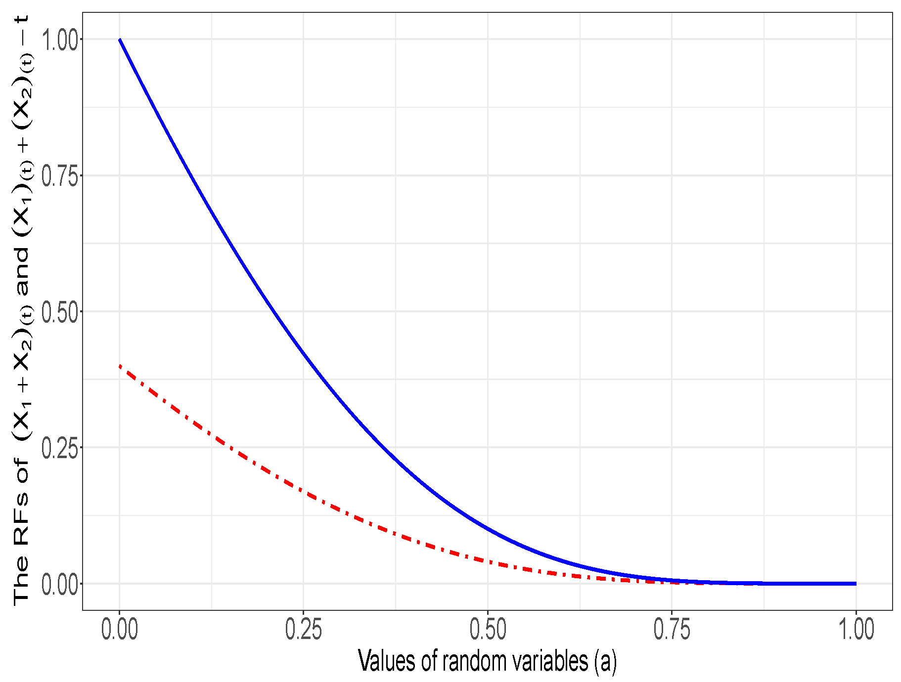
Example 2.

We say that X has a gamma distribution with shape parameter $\alpha >0$ and the scale parameter λ and denote it by $X\sim G(\alpha ,\lambda )$ whenever X has a PDF $f_X\left(x\right)=\frac{{\lambda }^{\alpha }{x}^{\alpha -1}{e}^{-\lambda x}}{\Gamma \left(\alpha \right)}$. Considering two lifetime organisms or devices working one after another in a system (a standby structure) and letting $X_i$ denote the lifetime of the ith organism, we can consider two situations for $i=1,2$: first, when both organisms fail before time $t=1$, and second when the system fails before time $t=1$. Suppose that $X_1\sim G(2,3)$ and $X_2\sim G(3,3)$. Note that if $X\sim G(k,\lambda )$, where $k\in \mathbb{N}$, the the CDF of X is derived via

$$F_X\left(x\right)=1-\sum _{n=0}^{k}exp(-\lambda x)\frac{{\left(\lambda x\right)}^n}{n!}.$$

(11)

Denote $P_4\left(a\right)=27a^4-144a^3+306a^2-312a+131$. In the spirit of the Equation (11), we find the CDF of the rv $W_2:={(X_1+X_2)}_{\left(t\right)}$ when $t=1$ as follows:

$$\begin{array}{cc}\hfill {\overline{F}}_{W_2}\left(a\right)& =\frac{{\int }_0^{1-a}{F}_{X_2}(1-a-x)f_{X_1}\left(x\right)dx}{{\int }_0^1{F}_{X_2}(1-x)f_{X_1}\left(x\right)dx}\hfill \\ \hfill & =\frac{P_4\left(a\right)exp\left(3(a-1)\right)-8}{131exp(-3)-8},\hfill \end{array}$$

On the other hand, from (11), the rv $V_2:={\left(X_1\right)}_{\left(t\right)}+{\left(X_2\right)}_{\left(t\right)}-t$ for $t=1$ has the following SF:

$$\begin{array}{cc}\hfill {\overline{F}}_{V_2}\left(a\right)& =\frac{{\int }_a^1{F}_{X_2}(x-a)f_{X_1}(1-x)dx}{F_{X_1}\left(1\right)F_{X_2}\left(1\right)}\hfill \\ \hfill & =\frac{P_4\left(a\right)exp\left(3a\right)-8exp\left(3\right)}{8(4-exp(3\left)\right)(68-exp(3\left)\right)}.\hfill \end{array}$$

From Theorem 1, $W_2{\ge }_{st}{V}_2$; thus, ${\overline{F}}_{W_2}\left(a\right)\ge {\overline{F}}_{V_2}\left(a\right)$ for all $a\in \mathbb{R}$. Figure 1 plots the graphs of ${\overline{F}}_{W_2}\left(a\right)$ and ${\overline{F}}_{V_2}\left(a\right)$ for $a\in [0,1]$ (for the values out of $[0,1]$, the ordering relation is obviously fulfilled) to exhibit the stochastic ordering property.

4.2. Likelihood Ratio Order-Based Bounds for the Idle Time of Cold Standby Systems with n Components

Before stating the next result, we need to introduce additional notation. We assume that $X_i\left(t\right):=t-{\left(X_i\right)}_{\left(t\right)}$, which is known in the literature as the past lifetime of $X_i,i=1,2$. Note that $X_i\left(t\right)$ has a distribution which corresponds to the conditional distribution of $X_i$, given that $X_i\le t$ for any $i=1,2$. In what follows, we take

$$\begin{array}{ccc}\hfill S_n& =& \sum _{i=1}^n{X}_i\hfill \\ \hfill S_{n\left(\mathit{t}\right)}& =& \sum _{i=1}^n{\left(X_i\right)}_{\left(t_i\right)}\hfill \\ \hfill {\left(S_n\right)}_{\left(t\right)}& =& (\sum _{i=1}^n{X}_i{)}_{\left(t\right)}\hfill \\ \hfill S_n\left(t\right)& =& \left(\sum _{i=1}^n{X}_i|\sum _{i=1}^n{X}_i\le t\right)\hfill \\ \hfill S_{n,\mathit{t}}& =& \sum _{i=1}^n{X}_i\left(t_i\right).\hfill \end{array}$$

In the following result, it is demonstrated that at a certain time t, for a cold standby system where the system and all the components in it are inactive, the overall idle time of the components is stochastically greater (with respect to likelihood ratio order) than the idle time of the cold standby unit.

Theorem 2.

Let $X_1,X_2,\dots ,X_n$ be independent rvs such that $X_n$ follows an exponential distribution with parameter ${\lambda }_n$. In addition, let ${\left(X_1\right)}_{\left(t\right)},{\left(X_2\right)}_{\left(t\right)},\dots ,{\left(X_n\right)}_{\left(t\right)}$ be independent for a fixed $t\ge 0$. Then,

$${(\sum _{i=1}^n{X}_i)}_{\left(t\right)}{\le }_{lr}\sum _{i=1}^n{\left(X_i\right)}_{\left(t\right)}.$$

Proof. 

Notice that ${\left(S_n\right)}_{\left(t\right)}:={\left({\sum }_{i=1}^n{X}_i\right)}_{\left(t\right)}$ has support $[0,t]$, while $S_{n\left(t\right)}:={\sum }_{i=1}^n{\left(X_i\right)}_{\left(t\right)}$ has support $[0,nt]$. Thus, we need to prove that $\frac{f_{S_{n\left(t\right)}}\left(s\right)}{f_{{\left(S_n\right)}_{\left(t\right)}}\left(s\right)}$ is increasing in $s\ge 0$ for every $s\le t$, as for $s>t$ we have $\frac{f_{S_{n\left(t\right)}}\left(s\right)}{f_{{\left(S_n\right)}_{\left(t\right)}}\left(s\right)}=+\infty$. Thus, we have

$$f_{{\left(S_n\right)}_{\left(t\right)}}\left(s\right)=\frac{f_{S_n}(t-s)}{F_{S_n}\left(t\right)}I[0\le s\le t],\mathrm{and}{f}_{S_{n\left(t\right)}}\left(s\right)={\int }_0^{+\infty }{f}_{{\left(X_n\right)}_{\left(t\right)}}(s-y)f_{S_{n-1\left(t\right)}}\left(y\right)dy.$$

Using Equation (6) and then applying the convolution formula on the density function of $S_n$, for every $s\in [0,t)$ we obtain

$$f_{{\left(S_n\right)}_{\left(t\right)}}\left(s\right)=\frac{f_{S_n}(t-s)}{F_{S_n}\left(t\right)}=\frac{{\int }_0^{+\infty }{f}_{X_n}(t-s-y)f_{S_{n-1}}\left(y\right)dy}{F_{S_n}\left(t\right)}.$$

Next, by imposing the convolution formula on the density function of $S_{n\left(t\right)}$, we have

$$f_{S_{n\left(t\right)}}\left(s\right)={\int }_0^{+\infty }{f}_{X_{n\left(t\right)}}(s-y)f_{S_{n-1\left(t\right)}}\left(y\right)dy.$$

Therefore,

$$\begin{array}{cc}\hfill \frac{f_{S_{n\left(t\right)}}\left(s\right)}{f_{{\left(S_n\right)}_{\left(t\right)}}\left(s\right)}& =F_{S_n}\left(t\right).\frac{{\int }_0^{+\infty }{f}_{X_{n\left(t\right)}}(s-y)f_{S_{n-1\left(t\right)}}\left(y\right)dy}{{\int }_0^{+\infty }{f}_{X_n}(t-s-y)f_{S_{n-1}}\left(y\right)dy}\hfill \\ \hfill & =\frac{F_{S_n}\left(t\right)}{F_{X_n}\left(t\right)}.\frac{{\int }_0^s{f}_{X_n}(t-s+y)f_{S_{n-1\left(t\right)}}\left(y\right)dy}{{\int }_0^{t-s}{f}_{X_n}(t-s-y)f_{S_{n-1}}\left(y\right)dy}\hfill \\ \hfill & =\frac{F_{S_n}\left(t\right)}{F_{X_n}\left(t\right)}.\frac{{\int }_0^s{f}_{X_n}(t-s+y)f_{S_{n-1\left(t\right)}}\left(y\right)dy}{{\int }_s^t{f}_{X_n}(u-s)f_{S_{n-1}}(t-u)du},\hfill \end{array}$$

where a change in the variable $u=t-y$ is made to derive the last equality. Because $X_n\sim E\left({\lambda }_n\right)$,

$$\begin{array}{cc}\hfill \frac{f_{S_{n\left(t\right)}}\left(s\right)}{f_{{\left(S_n\right)}_{\left(t\right)}}\left(s\right)}& =\frac{F_{S_n}\left(t\right)}{F_{X_n}\left(t\right)}.\frac{{\int }_0^s{\lambda }_{n}exp(-{\lambda }_n(t-s+y))f_{S_{n-1\left(t\right)}}\left(y\right)dy}{{\int }_s^t{\lambda }_{n}exp(-{\lambda }_n(u-s))f_{S_{n-1}}(t-u)du}\hfill \\ \hfill & =\frac{exp\left({\lambda }_{n}t\right).F_{S_n}\left(t\right)}{F_{X_n}\left(t\right)}.\frac{{\int }_0^{s}exp(-{\lambda }_{n}y)f_{S_{n-1\left(t\right)}}\left(y\right)dy}{{\int }_s^{t}exp(-{\lambda }_{n}u)f_{S_{n-1}}(t-u)du}.\hfill \end{array}$$

Hence, for all $0\le s\le t$ we obtain

$$\begin{array}{cc}\hfill \frac{\partial }{\partial s}log\left(\frac{f_{S_{n\left(t\right)}}\left(s\right)}{f_{{\left(S_n\right)}_{\left(t\right)}}\left(s\right)}\right)& =\frac{\partial }{\partial s}log\left(\frac{{\int }_0^{s}exp(-{\lambda }_{n}y)f_{S_{n-1\left(t\right)}}\left(y\right)dy}{{\int }_s^{t}exp(-{\lambda }_{n}u)f_{S_{n-1}}(t-u)du}\right)\hfill \\ \hfill & =\frac{exp(-{\lambda }_{n}s)f_{S_{n-1\left(t\right)}}\left(s\right)}{{\int }_0^{s}exp(-{\lambda }_{n}y)f_{S_{n-1\left(t\right)}}\left(y\right)dy}+\frac{exp(-{\lambda }_{n}s)f_{S_{n-1}}(t-s)}{{\int }_s^{t}exp(-{\lambda }_{n}y)f_{S_{n-1}}(t-y)dy},\hfill \end{array}$$

which is non-negative. Thus, the proof of theorem is completed. □

We provide a situation to examine the result of Theorem 2 in Example 3 below.

Example 3.

Suppose that $X_1\sim E\left(\lambda \right)$ and $X_2\sim E\left(2\lambda \right)$ with $\lambda >0$. Following Arnold and Villaseñor [48], we can deduce that $S_2:=X_1+X_2$ has a PDF

$$f_{S_2}\left(s\right)=2\lambda exp(-\lambda s)(1-exp(-\lambda s))$$

and CDF

$$F_{S_2}\left(s\right)=1-2exp(-\lambda s)+exp(-2\lambda s).$$

For all $w\in (0,t)$, the rv $W_2:={(X_1+X_2)}_{\left(t\right)}$ has a PDF

$$f_{W_2}\left(w\right)=\frac{2\lambda }{1-2exp(-\lambda t)+exp(-2\lambda t)}(exp(-\lambda (t-w))-exp(-2\lambda (t-w))).$$

The rv $W_3={\left(X_1\right)}_{\left(t\right)}+{\left(X_2\right)}_{\left(t\right)}$ has a PDF

$$f_{W_3}\left(w\right)=\frac{2\lambda exp(-3\lambda t)}{(1+exp(-\lambda t)){(1-exp(-\lambda t))}^2}(exp\left(2\lambda w\right)-exp\left(\lambda w\right)).$$

Therefore, $W_2{\le }_{lr}{W}_3$ if and only if

$$R_{\lambda }(w,t)=\frac{exp\left(2\lambda w\right)-exp\left(\lambda w\right)}{exp(-\lambda (t-w\left)\right)-exp(-2\lambda (t-w\left)\right)}.$$

Let us choose $\lambda =4$ and $t=2$. We show in Figure 2 that $R_4(w,2)$ is an increasing function. This confirms the result of Theorem 2.

Consider a cold standby system composed of a single component with a general continuous lifetime distribution equipped with one additional component with an exponential distribution lifetime. In this case, it can be realized from Theorem 2 that the idle time of the cold standby system is smaller with respect to the likelihood ratio order than the sum of the inactivity times of both components measured at a specified time t. Note that the time t is considered to be the time at which the system and its components are inactive and not functioning.

The following technical lemma is useful and is applied in the following.

Lemma 1.

Suppose that ${\tau }_1,{\tau }_2,\dots ,{\tau }_m$ are m points in time with a mean $\overline{\tau }$ and that $X_1,X_2,\dots ,X_m$ are m non-negative rvs; then, $m\overline{\tau }-\left(S_m\right)\left(m\overline{\tau }\right){=}_{st}{S}_{m\left(\mathit{\tau }\right)}$, where ${=}_{st}$ refers to the equality in the distribution.

Theorem 3.

Let $X_1,X_2,\dots X_m$ be independent non-negative rvs such that $X_1\left(t_1\right),X_2\left(t_2\right),\dots ,$$X_m\left(t_m\right)$ and $X_1\left({\tau }_1\right),X_2\left({\tau }_2\right),\dots ,$$X_n\left({\tau }_n\right)$, where $m>n$ are independent and where $t_1,t_2,\dots ,t_m$ are m fixed time points, and as such are ${\tau }_1,{\tau }_2,\dots ,{\tau }_n$. Let $X_i\in ILR,i=1,2,\dots ,n$, then if

(i) 

$m\overline{t}\ge n\overline{\tau }$, where $t_m\ge n\overline{\tau }$, in which $\overline{\tau }=\frac{{\sum }_{i=1}^n{\tau }_i}{n}$ and $\overline{t}=\frac{{\sum }_{i=1}^m{t}_i}{m}$,

(ii) 

$X_m$ and $X_n$ have identical distributions, and

(iii) 

${\sum }_{i=1}^{m-1}{X}_i\left(t_i\right){\ge }_{lr}{\sum }_{i=1}^n{X}_i$ for $t_i\ge 0,i=1,2,\dots ,m$,

We have

$${(\sum _{i=1}^n{X}_i)}_{\left(n\overline{\tau }\right)}{\ge }_{lr}\sum _{i=1}^m{\left(X_i\right)}_{\left(t_i\right)}-m\overline{t}+n\overline{\tau }.$$

(12)

Proof. 

We first prove that $S_n\left(n\overline{\tau }\right):=\left({\sum }_{i=1}^n{X}_i\right)\left(n\overline{\tau }\right){\le }_{lr}{\sum }_{i=1}^m{\left(X_i\right)}_{\left(t_i\right)}:=S_{m,\mathit{t}}$. The result is then proved following our discussions here. From Theorem 1.C.8 in Shaked and Shanthikumar [45], if $\psi$ is a decreasing function, then $X{\le }_{lr}Y$ implies that $\psi \left(X\right){\ge }_{lr}\psi \left(Y\right)$. Thus, if $\psi \left(x\right)=m\overline{t}-x$, because $S_n\left(n\overline{\tau }\right){\le }_{lr}{S}_{m,\mathit{t}}$, it follows that $m\overline{t}-S_n\left(n\overline{\tau }\right){\ge }_{lr}m\overline{t}-S_{m,\mathit{t}}$. Using Lemma 1, it can be realized that $m\overline{t}-S_n\left(n\overline{\tau }\right){=}_{st}m\overline{t}-n\overline{\tau }+{\left(S_n\right)}_{\left(n\overline{\tau }\right))}$, and in addition that $m\overline{t}-S_{m,\mathit{t}}{=}_{st}{S}_{m\left(\mathit{t}\right)}$. Hence, it follows that ${\left(S_n\right)}_{\left(n\overline{\tau }\right)}{\ge }_{lr}{S}_{m\left(\mathit{t}\right)}-m\overline{t}+n\overline{\tau }$. Thus, it is sufficient to prove that $\frac{f_{S_{m,\mathit{t}}}\left(s\right)}{f_{S_n\left(n\overline{\tau }\right)}\left(s\right)}$ is increasing in $0<s\le n\overline{\tau }$. We assume that $I[x\in A]$ is the indicator function of the set $[x\in A]$, which is equal to one if $x\in A$ and is equal to 0 if $x\in A^c$, where $A^c$ is the complement of the set A. For every $s\in (0,n\overline{\tau }]$, we can write

$$\begin{array}{cc}\hfill \frac{f_{S_{m,\mathit{t}}}\left(s\right)}{f_{S_n\left(n\overline{\tau }\right)}\left(s\right)}& =\frac{F_{S_n}\left(n\overline{\tau }\right){\int }_0^{+\infty }{f}_{X_m\left(t_m\right)}(s-y)f_{S_{m-1,\mathit{t}}}\left(y\right)dy}{{\int }_0^{+\infty }{f}_{X_n}(s-y)f_{S_{n-1}}\left(y\right)dy}\hfill \\ \hfill & =\frac{F_{S_n}\left(n\overline{\tau }\right)}{F_{X_m}\left(t_m\right)}.\frac{{\int }_0^{+\infty }{f}_{X_m}(s-y)I[s-y\le t_m]f_{S_{m-1,\mathit{t}}}\left(y\right)I[y>0]dy}{{\int }_0^{+\infty }{f}_{X_n}(s-y)f_{S_{n-1}}\left(y\right)dy}\hfill \\ \hfill & =\frac{F_{S_n}\left(n\overline{\tau }\right)}{F_{X_m}\left(t_m\right)}.\frac{{\int }_{(s-t_m)\vee 0}^{+\infty }{f}_{X_m}(s-y)f_{S_{m-1,\mathit{t}}}\left(y\right)dy}{{\int }_0^{+\infty }{f}_{X_n}(s-y)f_{S_{n-1}}\left(y\right)dy}\hfill \\ \hfill & =\frac{F_{S_n}\left(n\overline{\tau }\right)}{F_{X_m}\left(t_m\right)}.\frac{{\int }_0^{+\infty }{f}_{X_m}(s-y)f_{S_{m-1,\mathit{t}}}\left(y\right)dy}{{\int }_0^{+\infty }{f}_{X_n}(s-y)f_{S_{n-1}}\left(y\right)dy},\hfill \end{array}$$

where $a\vee b$ stands for the maximum of a and b and the last identity follows from the fact that for all $s\in (0,n\overline{t}]$, from assumption (i) above we have $s-t_m\le s-n\overline{t}\le 0$, meaning that $(s-t_m)\vee 0=0$. Therefore, because $X_m$ and $X_n$ are identical in distribution (assumption (ii)), for every $s\in (0,n\overline{t}]$ we have

$$\begin{array}{cc}\hfill \frac{f_{S_{m,\mathit{t}}}\left(s\right)}{f_{S_n\left(n\overline{\tau }\right)}\left(s\right)}& =\frac{F_{S_n}\left(n\overline{\tau }\right)}{F_{X_m}\left(t_m\right)}.{\int }_0^{+\infty }\frac{f_{X_m}(s-y)}{f_{X_n}(s-y)}.\frac{f_{S_{m-1,\mathit{t}}}\left(y\right)}{f_{S_{n-1}}\left(y\right)}\frac{f_{X_n}(s-y)f_{S_{n-1}}\left(y\right)}{{\int }_0^{+\infty }{f}_{X_n}(s-y)f_{S_{n-1}}\left(y\right)dy}dy\hfill \\ \hfill & =\frac{F_{S_n}\left(n\overline{\tau }\right)}{F_{X_m}\left(t_m\right)}{\int }_0^{+\infty }\frac{f_{S_{m-1,\mathit{t}}}\left(y\right)}{f_{S_{n-1}}\left(y\right)}{f}_{X_n|S_n=s}(s-y|s)dy\hfill \\ \hfill & =\frac{F_{S_n}\left(n\overline{\tau }\right)}{F_{X_m}\left(t_m\right)}{\int }_0^{+\infty }\Psi \left(y\right)f_{S_{n-1}|S_n=s}\left(y\right|s)dy\hfill \\ \hfill & =\frac{F_{S_n}\left(n\overline{\tau }\right)}{F_{X_m}\left(t_m\right)}E\left({\displaystyle \Psi \left(S_{n-1}\right)\mid S_n=s}\right),\hfill \end{array}$$

(13)

where $\Psi \left(y\right)=\frac{f_{S_{m-1,\mathit{t}}}\left(y\right)}{f_{S_{n-1}}\left(y\right)}$. From assumption (iii), $X_i\in ILR$ for all $i=1,2,\dots ,n$; thus, because the convolution of log-concave densities is log-concave, $S_{n-1}\in ILR$. From Theorem 1.C.53 of Shaked and Shanthikumar [45], we conclude that

$$\left[S_{n-1}\right|S_n=s_1]{\le }_{lr}\left[S_{n-1}\right|S_n=s_2],\mathrm{for}\mathrm{all}{s}_1\le s_2\in {\mathbb{R}}^{+},$$

Moreover, because ${\le }_{lr}$ implies that ${\le }_{st}$, we have

$$\left[S_{n-1}\right|S_n=s_1]{\le }_{st}\left[S_{n-1}\right|S_n=s_2]\mathrm{for}\mathrm{all}{s}_1\le s_2\in {\mathbb{R}}^{+}.$$

(14)

Furthermore, from assumption (iii), the function $\Psi \left(y\right)$ is increasing in $y>0$. From (13) and (14), it follows that $\frac{f_{S_{m,\mathit{t}}}\left(s\right)}{f_{S_n\left(n\overline{\tau }\right)}\left(s\right)}$ is increasing in $s>0$, which validates the proof. □

The following example shows that the conditions in Theorem 3 are accessible.

Example 4.

Choose $m=3$ and $n=2$ such that $t_1=1,t_2=2,t_3=1.5$ and ${\tau }_1=0.25,{\tau }_2=1$. It can be readily seen that $m\overline{t}>n\overline{\tau }$ and $t_m>n\overline{\tau }$, that is, condition (i) in Theorem 3 holds. Further, let $X_i\sim U(0,2),i=1,2,3$, i.e., the $X_i$s are distributed uniformly over $(0,2)$. Thus, $X_3$ and $X_2$ are equal in distribution, and condition (ii) in Theorem 3 is satisfied. It can be seen that $f_{X_i}\left(x\right)=I[0<x<2]/2$ is log-concave in x, i.e., $X_i\in ILR$, for all $i=1,2,3$; therefore, another sufficient condition in Theorem 3 holds true. It is not hard to prove that $X_i\left(t_i\right):=\left(X_i\right|X_i\le t_i)\sim U(0,t_i),i=1,2,3$. In addition, we can prove after calculation that

$$f_{X_1\left(t_1\right)+X_2\left(t_2\right)}\left(s\right)=\frac{s}{t_1{t}_2}·I[0<s\le t_1]+\frac{1}{t_2}·I[t_1<s\le t_2]+\frac{t_1+t_2-s}{t_1{t}_2}·I[t_2<s\le t_1+t_2].$$

It is easily observable that $f_{X_1\left(t_1\right)+X_2\left(t_2\right)}\left(s\right)/f_{X_1}\left(s\right)$ is non-decreasing in $s\in (0,2)$, meaning that condition (iii) in Theorem 3 is valid. Therefore, as follows from Theorem 3, we can conclude that the ordering relation provided in (12) is satisfied.

4.3. Further Bounds for the Idle Time of Cold Standby Systems with 2 Components

Cold standby systems with two components are very important in reliability and systems analysis. This is because redundancy methods usually assume that there is only one spare part for certain components of a given system with a specified structure, as the first unit is considered the main working unit and the second component the standby unit. The following lemma is useful in proving the next result.

Lemma 2.

Let $X_1,X_2,\dots ,X_m$ be m dependent rvs which are non-negative; further, let $X_i\left({\tau }_i\right),i=1,2,\dots ,m$ be independent. Then,

$$\sum _{i=1}^m{X}_i\left({\tau }_i\right){=}_{st}(\sum _{i=1}^m{X}_i\mid X_1\le {\tau }_1,\cdots ,X_m\le {\tau }_m),$$

in which ${\tau }_1,\dots ,{\tau }_m$ are m points of time such that ${\prod }_{i=1}^m{F}_{X_i}\left({\tau }_i\right)>0$.

Proof. 

It suffices to prove that $S_m\left(\mathit{\tau }\right):={\sum }_{i=1}^m{X}_i\left({\tau }_i\right)$ and $(S_m\mid X_i\le {\tau }_i,i=1,\dots ,m)$ have a common moment generating function. Denote $\mathit{X}=(X_1,\dots ,X_m)$ and let $\left(\mathit{X}\right|X_i\le {\tau }_i,i=1,\dots ,m)$ have a conditional PDF $f_{\left(\mathit{X}\right|X_i\le {\tau }_i,i=1,\dots ,m)}$. Because the $X_i$s are independent, for all $\mathit{x}=(x_1,\dots ,x_m)\in {\mathbb{R}}^m$ we have

$$\begin{array}{cc}\hfill f_{\left(\mathit{X}\right|X_i\le {\tau }_i,i=1,\dots ,m)}(x_1,\dots ,x_m)& =\frac{f_{\mathit{X}}\left(\mathit{x}\right).I[x_1\le {\tau }_1,\dots ,x_m\le {\tau }_m]}{P(X_1\le {\tau }_1,\cdots ,X_m\le {\tau }_m)}\hfill \\ \hfill & =\prod _{i=1}^m\left(\frac{f_{X_i}\left(x_i\right)}{F_{X_i}\left({\tau }_i\right)}\right)I[x_1\le {\tau }_1,\dots ,x_m\le {\tau }_m].\hfill \end{array}$$

Now, we can write

$$\begin{array}{cc}\hfill M_{(S_m\mid X_i\le {\tau }_i,i=1,\dots ,m)}\left(t\right)& =E(exp\left(t{S}_m\right)|X_i\le {\tau }_i,i=1,\dots ,m)\hfill \\ \hfill & =E(\prod _{i=1}^{m}exp\left(t{X}_i\right)\mid X_i\le {\tau }_i,i=1,\dots ,m)\hfill \\ \hfill & ={\int }_0^{+\infty }\cdots {\int }_0^{+\infty }\left(\prod _{i=1}^{m}exp\left(t{x}_i\right)\right)f_{\left(\mathit{X}\right|X_i\le {\tau }_i,i=1,\dots ,m)}(x_1,\dots ,x_m)d{x}_m\dots d{x}_1\hfill \\ \hfill & ={\int }_0^{{\tau }_1}\cdots {\int }_0^{{\tau }_m}\prod _{i=1}^m\left(exp\left(t{x}_i\right)\frac{f_{X_i}\left(x_i\right)}{F_{X_i}\left({\tau }_i\right)}\right)\hfill \\ \hfill & =\prod _{i=1}^m\left({\int }_0^{{\tau }_i}\frac{exp\left(t{x}_i\right)f_{X_i}\left(x_i\right)}{F_{X_i}\left({\tau }_i\right)}d{x}_i\right)\hfill \\ \hfill & =\prod _{i=1}^{m}E(exp\left(t{X}_i\left({\tau }_i\right)\right))\hfill \\ \hfill & =M_{S_m\left(\mathit{\tau }\right)}\left(t\right),forallt\in \mathbb{R},\hfill \end{array}$$

where the last identity follows from the assumption that $X_1\left({\tau }_1\right),\cdots ,X_m\left({\tau }_m\right)$ are independent. The proof is completed. □

The following result presents a sufficient condition for the usual stochastic ordering between the idle time of an inactive standby system of size two and the sum of the idle times of the inactive components. It is worth mentioning that as standby systems of size two are very important as an effective redundancy method in engineering reliability systems, the previous results are of particular interest when $n=2$.

Theorem 4.

Let $X_1$ and $X_2$ be two independent rvs such that ${\left(X_1\right)}_{\left({\tau }_1\right)}$ and ${\left(X_2\right)}_{\left({\tau }_2\right)}$ are independent for ${\tau }_1\le {\tau }_2$ as two specified points of time. Suppose that ${\tilde{h}}_{X_2}(s-{\tau }_1)\le {\tilde{h}}_{X_1+X_2}\left(s\right),$ for all $s\in [{\tau }_1,{\tau }_1+{\tau }_2]$; then,

$${(X_1+X_2)}_{({\tau }_1+{\tau }_2)}{\le }_{st}{\left(X_1\right)}_{\left({\tau }_1\right)}+{\left(X_2\right)}_{\left({\tau }_2\right)}.$$

Proof. 

In a similar manner as in the proof of Theorem 3, it is sufficient to show that $\left(S_2\right)({\tau }_1+{\tau }_2){\ge }_{st}{S}_{2,\mathit{\tau }}$. From Lemma 2, when $m=2$, because $X_1$ and $X_2$ as well as $X_1\left({\tau }_1\right)$ and $X_2\left({\tau }_2\right)$ are independent, we have $S_{2,\mathit{\tau }}{=}_{st}(S_2\mid X_1\le {\tau }_1,X_2\le {\tau }_2)$. Thus, we can prove that

$$\left(S_2\right)({\tau }_1+{\tau }_2){\ge }_{st}(S_2\mid X_1\le {\tau }_1,X_2\le {\tau }_2).$$

(15)

By routine calculation, it is evident that (15) is satisfied if and only if

$$P(S_2\le s\mid S_2\le {\tau }_1+{\tau }_2)\le P(S_2\le s\mid X_1\le {\tau }_1,X_2\le {\tau }_2),\mathrm{for}\mathrm{all}s\in (0,{\tau }_1+{\tau }_2],$$

which holds if and only if

$$P(X_1\le {\tau }_1,X_2\le {\tau }_2\mid S_2\le {\tau }_1+{\tau }_2)\le P(X_1\le {\tau }_1,X_2\le {\tau }_2\mid S_2\le s)\mathrm{for}\mathrm{all}s\in (0,{\tau }_1+{\tau }_2].$$

(16)

The inequality in (16) holds true for $s\in (0,{\tau }_1]$, as it can be obviously seen that

$$\begin{array}{cc}\hfill P(X_1\le {\tau }_1,X_2\le {\tau }_2\mid S_2\le {\tau }_1+{\tau }_2)& =\frac{P(X_1\le {\tau }_1,X_2\le {\tau }_2)}{P(S_2\le {\tau }_1+{\tau }_2)}\hfill \\ \hfill & \le \frac{P(X_1\le {\tau }_1,X_2\le {\tau }_2)}{P(S_2\le s)}\hfill \\ \hfill & =P(X_1\le {\tau }_1,X_2\le {\tau }_2\mid S_2\le s).\hfill \end{array}$$

Thus, we only need to prove that the inequality in (16) is satisfied for $s\in ({\tau }_1,{\tau }_1+{\tau }_2]$. Note that

$$\begin{array}{cc}\hfill {\int }_0^{{\tau }_2}\frac{f_{X_2}\left(x_2\right)I[x_2\le s-x_1]}{F_{S_2}\left(s\right)}d{x}_2& =P(X_2(s-x_1)\le {\tau }_2)F_{X_2}(s-x_1)\hfill \\ \hfill & =F_{X_2}((s-x_1)\wedge {\tau }_2),\hfill \end{array}$$

where $a\wedge b=min\{a,b\}$. Thus, we can obtain

$$\begin{array}{cc}\hfill P(X_1\le {\tau }_1,X_2\le {\tau }_2\mid S_2\le s)& ={\int }_0^{{\tau }_1}{\int }_0^{{\tau }_2}\frac{f_{X_1}\left(x_1\right)f_{X_2}\left(x_2\right)I[x_1+x_2\le s]}{F_{X_1+X_2}\left(s\right)}d{x}_{2}d{x}_1\hfill \\ \hfill & ={\int }_0^{{\tau }_1}{f}_{X_1}\left(x_1\right)\left({\int }_0^{{\tau }_2}\frac{f_{X_2}\left(x_2\right)I[x_2\le s-x_1]}{F_{X_1+X_2}\left(s\right)}d{x}_2\right)d{x}_1\hfill \\ \hfill & ={\int }_0^{{\tau }_1}{f}_{X_1}\left(x_1\right)\frac{F_{X_2}((s-x_1)\wedge {\tau }_2)}{F_{X_1+X_2}\left(s\right)}d{x}_1.\hfill \end{array}$$

Therefore, to prove (15) it is sufficient to show the following for all $s\in ({\tau }_1,{\tau }_1+{\tau }_2]$:

$${\int }_0^{{\tau }_1}{f}_{X_1}\left(x_1\right)\frac{F_{X_2}((s-x_1)\wedge {\tau }_2)}{F_{S_2}\left(s\right)}d{x}_1\ge {\int }_0^{{\tau }_1}{f}_{X_1}\left(x_1\right)\frac{F_{X_2}(({\tau }_1+{\tau }_2-x_1)\wedge {\tau }_2)}{F_{S_2}({\tau }_1+{\tau }_2)}d{x}_1.$$

Because we have $({\tau }_1+{\tau }_2-x_1)\wedge {\tau }_2={\tau }_2$ for all $x_1\le {\tau }_1$, it suffices to prove that

$${\int }_0^{{\tau }_1}{f}_{X_1}\left(x_1\right)\frac{F_{X_2}((s-x_1)\wedge {\tau }_2)}{F_{S_2}\left(s\right)}d{x}_1\ge {\int }_0^{{\tau }_1}{f}_{X_1}\left(x_1\right)\frac{F_{X_2}\left({\tau }_2\right)}{F_{S_2}({\tau }_1+{\tau }_2)}d{x}_1$$

holds for all $s\in ({\tau }_1,{\tau }_1+{\tau }_2]$, that is, it is enough to demonstrate that for all $s\in ({\tau }_1,{\tau }_1+{\tau }_2]$ we have

$${\int }_0^{{\tau }_1}{f}_{X_1}\left(x_1\right)\mathsf{\Phi }(x_1,s,{\tau }_1,{\tau }_2)d{x}_1\ge 0,$$

where

$$\mathsf{\Phi }(x_1,s,{\tau }_1,{\tau }_2)=\left[\frac{F_{X_2}((s-x_1)\wedge {\tau }_2)}{F_{S_2}\left(s\right)}-\frac{F_{X_2}\left({\tau }_2\right)}{F_{S_2}({\tau }_1+{\tau }_2)}\right].$$

Let us assume that ${\tau }_1\le s<{\tau }_2$; then, we can show that

$${\int }_0^{{\tau }_1}{f}_{X_1}\left(x\right)\Psi (x_1,s,{\tau }_1,{\tau }_2)d{x}_1\ge 0,\mathrm{for}\mathrm{all}s\in [{\tau }_1,{\tau }_2).$$

Because $s<{\tau }_2$, it is the case that $s-x_1\le {\tau }_2-x_1\le {\tau }_2$ for all $x_1\in (0,{\tau }_1)$; hence, $(s-x_1)\wedge {\tau }_2=s-x_1$. Therefore,

$$\begin{array}{cc}\hfill \Psi (x_1,s,{\tau }_1,{\tau }_2)& =\left[\frac{F_{X_2}(s-x_1)}{F_{S_2}\left(s\right)}-\frac{F_{X_2}\left({\tau }_2\right)}{F_{S_2}({\tau }_1+{\tau }_2)}\right]\hfill \\ \hfill & \ge \left[\frac{F_{X_2}(s-{\tau }_1)}{F_{S_2}\left(s\right)}-\frac{F_{X_2}\left({\tau }_2\right)}{F_{S_2}({\tau }_1+{\tau }_2)}\right],\hfill \end{array}$$

which is non-negative if $\frac{F_{X_2}(s-{\tau }_1)}{F_{S_2}\left(s\right)}$ is decreasing in $s\in [{\tau }_1,{\tau }_2)$. This is additionally satisfied if the assumption that ${\tilde{h}}_{X_2}(s-{\tau }_1)\le {\tilde{h}}_{X_1+X_2}\left(s\right)$ for all $s\in [{\tau }_1,{\tau }_1+{\tau }_2]$ holds. Now, assuming that ${\tau }_2\le s<{\tau }_1+{\tau }_2$,

$${\int }_0^{s-{\tau }_2}\Psi (x_1,s,{\tau }_1,{\tau }_2)d{x}_1\ge {\int }_0^{s-{\tau }_2}{F}_{X_2}\left({\tau }_2\right)f_{X_1}\left(x_1\right)\left(\frac{1}{F_{S_2}\left(s\right)}-\frac{1}{F_{S_2}({\tau }_1+{\tau }_2)}\right)d{x}_1\ge 0.$$

In a similar manner to the case when ${\tau }_1\le s_2<{\tau }_2$, we can now establish that

$${\int }_{s-{\tau }_2}^{{\tau }_1}\Psi (x_1,s,{\tau }_1,{\tau }_2)d{x}_1\ge 0.$$

As a result, we have ${\int }_0^{{\tau }_1}\Psi (x_1,s,{\tau }_1,{\tau }_2)d{x}_1\ge 0$ for all $s\in [{\tau }_2,{\tau }_1+{\tau }_2]$. The proof of the theorem is now completed. □

In the context of the conditions of Theorem 4, it is possible to question whether the assumption that ${\tilde{h}}_{X_2}(s-{\tau }_1)\le {\tilde{h}}_{X_1+X_2}\left(s\right)$ for all $s\in [{\tau }_1,{\tau }_1+{\tau }_2]$ is attainable. The following remark clarifies this issue.

Remark 1.

Suppose that $X_1$ and $X_2$ respectively represent the lifetime of a component and the lifetime of the standby unit which, are assumed to be independent. Note that for all $x<0$ we have $f_{X_i}\left(x\right)=F_{X_i}\left(x\right)=0,i=1,2$. We can write

$$\begin{array}{cc}\hfill {\tilde{h}}_{X_1+X_2}\left(s\right)& :=\frac{f_{X_1+X_2}\left(s\right)}{F_{X_1+X_2}\left(s\right)}\hfill \\ \hfill & =\frac{{\int }_0^{+\infty }{f}_{X_2}(s-x_1)f_{X_1}\left(x_1\right)d{x}_1}{{\int }_0^{+\infty }{F}_{X_2}(s-x_1)f_{X_1}\left(x_1\right)d{x}_1}\hfill \\ \hfill & ={\int }_0^s\frac{f_{X_2}(s-x_1)}{F_{X_2}(s-x_1)}\frac{F_{X_2}(s-x_1)f_{X_1}\left(x_1\right)}{{\int }_0^{+\infty }{F}_{X_2}(s-x_1)f_{X_1}\left(x_1\right)d{x}_1}d{x}_1\hfill \\ \hfill & ={\int }_0^s{\tilde{h}}_{X_2}(s-x_1)f^{\star }\left(x_1\right|s)d{x}_1\hfill \\ \hfill & =E\left[{\tilde{h}}_{X_2}(s-X_s^{\star })\right],\hfill \end{array}$$

where $X_s^{\star }$ is a non-negative rv with a PDF $f^{\star }(·|s)$ provided by

$$f^{\star }\left(x_1\right|s)=\frac{F_{X_2}(s-x_1)f_{X_1}\left(x_1\right)}{{\int }_0^{+\infty }{F}_{X_2}(s-x_1)f_{X_1}\left(x_1\right)d{x}_1}.$$

(17)

Note that $E\left(X_s^{*}\right)\le s$. Now, consider an $s_0>0$ such that $s_0<s<{\tau }_1+{\tau }_2$ and for which ${\tau }_1=E\left(X_{s_0}^{*}\right)\le E\left(X_s^{*}\right)$. Supposing that $X_2$ has a decreasing convex reversed hazard rate function, on using Jensen’s inequality, for all $s<{\tau }_1+{\tau }_2$ we have

$$\begin{array}{cc}\hfill {\tilde{h}}_{X_1+X_2}\left(s\right)& =E\left[{\tilde{h}}_{X_2}(s-X_s^{\star })\right],\hfill \\ \hfill & \ge {\tilde{h}}_{X_2}(s-E\left(X_s^{\star }\right)),\hfill \\ \hfill & \ge {\tilde{h}}_{X_2}(s-{\tau }_1).\hfill \end{array}$$

Now, Theorem 4 is applicable, as the sufficient condition of this theorem is satisfied.

We provide the next example to fulfill the conditions in Theorem 4 in the case of heterogenous exponential components.

Example 5.

Suppose that $X_1$ and $X_2$ have an exponential distribution with parameters ${\lambda }_1$ and ${\lambda }_2$, respectively. It can be checked that the reversed hazard rate function of exponential distribution is decreasing and convex. Thus, ${\tilde{h}}_{X_2}\left(x\right)=\frac{{\lambda }_2}{exp\left({\lambda }_{2}x\right)-1}$ is a decreasing function in x which is further convex in x. The rv $X_s^{\star }$, as introduced in Remark 1 with PDF (17), has a PDF

$$f^{\star }\left(x_1\right|s)=\frac{exp(-{\lambda }_{1}x)-exp(-{\lambda }_{2}s+({\lambda }_2-{\lambda }_1)x)}{\frac{1}{{\lambda }_1}(1-exp(-{\lambda }_{1}s))+\frac{1}{{\lambda }_2-{\lambda }_1}(exp(-{\lambda }_{2}s)-exp(-{\lambda }_{1}s))},0\le x\le s.$$

It is straightforward that if $X_2\in DRHR$, then $F_{X_2}(s-x_1)$ is $T{P}_2$ in $(x_1,s)\in {\mathbb{R}}^{+}\times {\mathbb{R}}^{+}$. As a result, from (17), $f^{*}\left(x_1\right|s)$ is $T{P}_2$ in $(x_1,s)\in {\mathbb{R}}^{+}\times {\mathbb{R}}^{+}$, that is, $X_{s_1}^{*}{\le }_{lr}{X}_{s_2}^{*}$ for every $0<s_1\le s_2$. Because ${\le }_{lr}$ implies ${\le }_{st}$, we can conclude that $X_{s_1}^{*}{\le }_{st}{X}_{s_2}^{*}$ for all $0<s_1\le s_2$. Therefore, $E\left(X_{s_1}^{*}\right)\le E\left(X_{s_2}^{*}\right)$ for all $s_1\le s_2\in {\mathbb{R}}^{+}$. For example, if ${\lambda }_1=2$ and ${\lambda }_2=3$, then after calculation we can obtain

$$E\left(X_s^{\star }\right)=\frac{exp\left(3s\right)+(3-6s)exp\left(s\right)-4}{2exp\left(3s\right)-6exp\left(s\right)+4},$$

which is an increasing function. Hence, if one chooses ${\tau }_1=E\left(X_0^{*}\right)=0$, following the discussion in Remark 1 and noting that for all $s>{\tau }_1$ we have $E\left(X_s^{*}\right)\ge E\left(X_{{\tau }_1}^{*}\right)\ge 0$, the assumption in Theorem 4 that ${\tilde{h}}_{X_2}(s-{\tau }_1)\le {\tilde{h}}_{X_1+X_2}\left(s\right)$ for all $s\in [{\tau }_1,{\tau }_1+{\tau }_2]$ is fulfilled on this account, and consequently, ${(X_1+X_2)}_{({\tau }_1+{\tau }_2)}{\le }_{st}{\left(X_1\right)}_{\left({\tau }_1\right)}+{\left(X_2\right)}_{\left({\tau }_2\right)}$, or more accurately, ${(X_1+X_2)}_{\left({\tau }_2\right)}{\le }_{st}{\left(X_2\right)}_{\left({\tau }_2\right)}$.

Before concluding the paper, we would like to point out that the study conducted in this paper has a number of limitations. For example, the random variables representing the component lifetime in a cold standby system are considered to be independent. In the literature, this condition is usually associated with the problem of convolution of random variables. There is another limitation to the research conducted in this study, namely, that we considered general cold standby systems and not specific ones installed in a particular interconnected system (e.g., systems with parallel or series structures containing redundant standby units). This could represent helpful approach to determine whether the results of the present work are useful for coherent systems as well.

5. Conclusions

In this study, we have presented results for obtaining upper and lower stochastic bounds for the idle time of standby systems after their failure in the context of random lifetimes. These bounds are in fact functions of the idle times of the components of the standby system. In this way, it is possible to evaluate whether it is reasonable to equip a component with redundant standby units in order to minimize the idle time of a standby system. We used two informative and commonly applied stochastic orderings, namely, the likelihood ratio ordering and the usual stochastic ordering. The problem of maintaining systems and replacing them with new systems, along with the similar problem of tuning their components, plays an important role in reliability engineering. This is because there are certain systems, e.g., systems that gradually fail under certain degradation processes, that need to be in operation uniformly, and it is very beneficial for such systems to have less idle time. The results obtained in this work may be useful in identifying situations where the idle time of inactive standby systems and the idle time of components in the system (or a function thereof) have a stochastic ordering property. Because the number of standby units can play a key role in reducing or even increasing costs and preventing further losses due to early component failures, it becomes increasingly important to identify whether a standby system is highly survivable, or equivalently whether it has lower inactivity compared to components that failed earlier.

In future additions to this study, we intend to consider two standby systems with different component lifetimes and possibly different numbers of components, and to investigate stochastic comparisons between the idle time of one system and the sum of the idle times of the components in the other system. We intend to look for the conditions for stochastic comparisons between the idle times of two standby systems. To provide further guidance for future research, the results of this paper can be taken up and, for example, the upper or lower bounds obtained in this paper for the idle time of standby systems can be considered to obtain sharper bounds.