Abstract
The authors develop the theory of discrete differentiation and, on its basis, solve the problem of detecting trends in records, using the idea of the connection between trends and derivatives in classical analysis but implementing it using fuzzy logic methods. The solution to this problem is carried out by constructing fuzzy measures of the trend and extremum for a recording. The theoretical justification of the regression approach to classical differentiation in the continuous case given in this work provides an answer to the question of what discrete differentiation is, which is used in constructing fuzzy measures of the trend and extremum. The detection of trends using trend and extremum measures is more stable and of higher quality than using traditional data analysis methods, which consist in studying the intervals of constant sign of the derivative for a piecewise smooth approximation of the original record. The approach proposed by the authors, due to its implementation within the framework of fuzzy logic, is largely focused on the researcher analyzing the record and at the same time uses the idea of multiscale. The latter circumstance provides a more complete and in-depth understanding of the process behind the recording.
Keywords:
trend problem; discrete regression derivatives; trend measures; extremum measures; multiscale; extremum migration MSC:
26E50
1. Introduction
Research on data and methods of their analysis using fuzzy mathematics has now taken shape as an independent direction, which includes methods of fuzzy regression and the analysis of fuzzy time series [1,2,3,4,5,6,7]. We can highlight the main stages of development of this direction.
In the initial stage, studies of the fuzzy regression model were carried out. The second stage was the development of soft-computing methods, within which a huge number of studies have been carried out on the effectiveness of soft computing for time series analysis. The third stage consisted in the transition from the analysis of time series using fuzzy mathematics methods to the analysis of fuzzy time series. The development of fuzzy database methods has made it possible to move to the stage of extracting rules from fuzzy (granular) time series.
Within each of the listed stages, a significant part consists of methods for identifying trends and, more broadly, a morphological analysis of time series. The proposed work should be attributed to the use of fuzzy mathematics methods for the analysis of discrete time series.
1.1. Trends and Fuzzy Principles for Their Modeling
Trends in a time series are its fundamental characteristic and therefore can tell a lot about the nature of the process behind it. The identification of trends is a significant part of what is traditionally considered to be the morphological analysis of time series [8,9,10,11], including:
- The decomposition of the time series into trend and seasonal components, as well as the remainder: the trend shows the general direction of changes over time, seasonality reflects repeating patterns associated with certain periods of time, and the remainder reflects random fluctuations within the time series;
- An autocorrelation analysis, which helps identify periodic fluctuations associated with seasonality;
- A spectral analysis, which allows one to analyze the cyclicity in a time series and the most important time periods for it.
Currently, a broader understanding of morphological analysis as the study of the manifestation of one or another geometric property in a graphical representation of the dynamics of a time series is gaining momentum [12]. A morphological analysis of time series is useful for a better understanding of their dynamics and more accurate forecasting.
There are several methods for constructing and identifying time series trends. Here are the main ones [8,11,13,14,15,16,17,18]: smoothing with a kernel (in particular, the moving average method, exponential smoothing), regression and autoregressive (AR) methods, wavelet analysis, nonlinear methods (in particular, machine learning and neural networks).
Real trends are stochastic and are not at all similar to ideal mathematical ones, since they have glitches. This does not confuse the researcher, who perceives the trend adaptively and understands when a violation is insignificant and the trend continues, and when a violation interrupts the trend.
Thus, if mathematical trends are strict and unambiguous segments in each subsequent node for which the value of the record is greater than, or equal to (less than, or equal to) the value of the record in the present node, then stochastic ones depend on the point of view of the researcher and therefore can differ.
Let us call the formalization and search for trends and extrema in a function the trend problem. Its solution, according to the authors, consists of a sequence of answers to the following questions:
- What is the trend of a function at a point?
- Which parts of the function should be considered definitely trendy?
- How do these fragments form a general trend?
- What is an extremum of a function?
The solution to the trend problem, according to the authors, should be fuzzy, multiparameter and multiscale in the spirit of wavelets and fractals. By changing the parameters and scale, the researcher gets a complete picture of the trends and selects the ones they need. In addition, a multiscale trend analysis is very useful, objective and can tell a lot about the function as a whole.
The above is fully consistent with the principles of fuzzy modeling, on the basis of which it is supposed to approach stochastic trends. In this regard, we quote Zadeh [19]: “All we need to solve most practical problems is a parameterized family of definitions that, if necessary, would allow a non-standard choice of operators that reflect the characteristic features of a particular application. The advantage of this approach is that by avoiding fixed, concrete-independent definitions, fuzzy set theory and fuzzy logic achieve a pluralism that increases their flexibility and expressive capabilities”.
In this work, such operators will be regression differentiation, regression smoothing, fuzzy trend measure and fuzzy extremum measure.
It should be noted that regression derivatives were used earlier, in a simpler form than in this work, for the classification of time series, which made it possible to determine groups of series similar in morphology using various similarity measures [20,21,22,23,24]. In such problems, the choice of similarity measure affects the classification accuracy to a greater extent than the choice of classification method.
The advantage of similarity measures constructed using regression derivatives is the ability to take into account both positive dependencies, when time series simultaneously increase or decrease values, and negative dependencies, when the values of one time series decrease and another increase, and vice versa [23]. Similar results based on the fuzzy correlation measure constructed by the authors are given in the conclusion.
1.2. Solution of the Problem of Trends and on the Basis of Discrete Mathematical Analysis
The problem of trends (see Section 1.1) in this work is solved within the framework of discrete mathematical analysis (DMA)—a new approach to data analysis, researcher-oriented and occupying an intermediate position between hard mathematical methods and soft intellectual ones [25,26,27,28,29].
The solution to the problem within the framework of DMA consists of two parts. The first is informal: it explains the researcher’s logic, introduces the necessary concepts, and explains the scheme and principles of the solution. The second is of a formal nature: with the help of the DMA apparatus, all concepts receive strict definitions within the framework of fuzzy mathematics and fuzzy logic, and the scheme and principles become algorithms.
We call the first, informal part of solving the trend problem within the framework of DMA the logic of the researcher’s trends (RTL) and formulate it in the form of the following provisions:
- There is a record f on a finite uniform set of nodes T. At each node, the researcher vaguely but unambiguously sees a positive, negative or neutral trend f.
- The researcher considers positive (negative) trends for f to be segments in T consisting of positive and neutral (negative and neutral) nodes from T.
- Opposite trends intersect at neutral nodes, among which the researcher can choose an extremum for f.
The further, main part of the work is devoted to the transformation of RTL into algorithms (the second part of solving the problem of trends within the framework of DMA): fuzzy measures of the trend and extremum are constructed, expressing the researcher’s opinion about the presence of a trend and extremum in a record in a particular node. The combined use of these measures makes it possible in a discrete situation to repeat the classical results of mathematical analysis regarding trends and extrema for piecewise smooth functions.
The measures are based on discrete regression derivatives. Their definition, study and rationale for use are given below. Having a discrete derivative, there is a natural desire to repeat on its basis, in a discrete situation, the scheme of the approach of classical mathematical analysis to trends and extremes. This determines both the motivation and goals of this work.
1.3. Regression Approach to Derivatives (Continuous Case)
Let the function f be integrable on an interval I containing zero internally. Then, for a sufficiently small , the segment is contained in I. Let us denote by the restriction of f to the segment : and calculate the projection of the function in space into the two-dimensional subspace of linear functions .
Statement 1.
If a function f has a tangent at zero, then, as , the linear projection tends to it.
Proof.
Let , be an orthonormal basis in , obtained from the natural basis by a Gram–Schmidt orthogonalization [30], then:
Let us put , . Three conditions arise on a, b and c:
Thus,
Additionally, the function f is differentiable at zero:
where when .
The limit
in the free term of the projection is explained by the mean value theorem [31].
Let us analyze the expansion coefficient at x:
The last integral tends to zero as :
□
1.4. Regression Approach to Derivatives (Discrete Case)
We postpone the consequences of the proven statement and its further development in the continuous case until the Appendix A, and now we discuss its significance mainly for the analysis of data in a discrete situation.
Replacing the tangent to f with the projection for small makes it possible to determine the tangent for discrete functions, since the projection is nothing more than a linear regression for f on and can be generalized to the discrete case.
The limit transition in the discrete case is replaced by a fuzzy weight structure of proximity to node t in a finite set of nodes T, the domain of definition of the function f.
The proven statement gives grounds to consider the linear regression of the function f with respect to the weight structure on T as a tangent for f at t, and its slope as the derivative of f at t.
Having a derivative for f, there is a natural desire to repeat on its basis in a discrete situation the classical approach to trends and extrema from mathematical analysis.
2. Discrete Regression Derivatives
Statement 1 proved above allows us to conclude that for a function f that is differentiable at zero, its linear continuous regressions on the segments tend to the tangent as .
This approach to differentiation in the continuous case allows a continuation to the discrete case, since discrete regressions are just as efficient and fundamental as continuous ones.
Let be a finite discrete segment with equal nodes , , .
Let us call a segment in T a piece in T without gaps: for some . In addition, we call the beginning (end) and denote by () the first and last nodes and , respectively.
We consider any real function on T to be a time series (record) f; is the space of such functions.
The analysis by a researcher of the behavior of a time series involves considering its values not only in a separate node but also simultaneously taking into account the values in some of its vicinity. This is precisely why the segment T needs to be localized at each of its nodes. It can be implemented using the fuzzy structure on T, which plays the role of a neighborhood of node t and expresses the proximity to it of individual nodes normalized in t: is a measure of theproximity of to t.
We consider the proximity measure on T to be a set of fuzzy structures : , .
The measure is the only parameter in the theory of trends and extrema constructed below and is therefore very important. Its choice is entirely determined by the researcher. The authors’ choice is the family .
Definition 1.
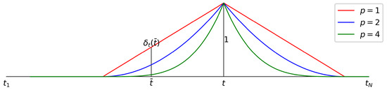
, p—scale parameter, r—viewing radius (Figure 1).
Figure 1.
Proximity of to node t for different p’s.
The family expresses the authors’ point of view on localization: a researcher analyzing a record f at node t first selects the boundary of the view (parameter r) and then its thoroughness (scale, parameter p). The required localization can be achieved using the family in two ways: either by the parameter r tending to zero, or by the parameter p tending to infinity. In this paper, the authors chose the second path: in the measure , there is an interesting dependence on the scale parameter p, which allows you to “look at the record from a different height”.
The parameters p and r are chosen by the researcher. In this work, the measure is used for trend analysis, which can be simple (p and r are fixed) and multiscale (p changes, r is fixed). The work focuses on multiscale analysis. For its objectivity and completeness, the radius r is assumed to be equal to a quarter of the length of the segment T. Figure 1 shows the dependence of the proximity to node t on p for r equal to a quarter of the length of the segment T.
The limit transition to T performs a proximity measure by distributing weights on T: . With that said, we should consider a linear regression based on the fuzzy image at the beginning of the tangent to the function f at node t. Associated with the image is the functional
The values of the parameters of the tangent are the minimum point of . Therefore, and satisfy the system of equations
Hence,
To build trends, the formulas in (3) are used. A simpler expression for and is used in Appendix A.1.
Definition 2.
The slope coefficient is called the regression derivative of f at t and is denoted by . The function is called the regression derivative of f and is denoted by . The functional correspondence is a linear operator on , called regression differentiation and denoted by .
Definition 3.
The value of the regression tangent of the function f at t is called the regression value of f at t and is denoted . The function is called regression smoothing of f and is denoted by . The functional correspondence is a linear operator on , called regression smoothing and denoted by .
A special notation for differentiation and smoothing in the case of a measure is:
The theoretical justification for the regression approach to differentiation presented in this work finds additional empirical confirmation in the form of the good performance of regression smoothing: with the same review (parameter p) on smooth functions, regression smoothing works better than conventional averaging. In Figure 2, regression smoothing is shown with a solid line, and conventional averaging is shown with a dotted line. The visual comparison is supported by the quadratic discrepancy with the ideal. The advantage of regression smoothing over conventional smoothing is especially visible at the ends of both the synthetic smooth recording (Figure 2) and the real one (Figure 3). Until the end of this paper, these records participate in the game and serve as a testing ground for the trends and extremes proposed in this work.
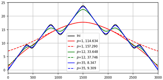
Figure 2.
Results of smoothing (solid line) and averaging (dotted line) for smooth records (black line) at different scales p with quadratic residuals deviations: (red lines), (green) and (blue).
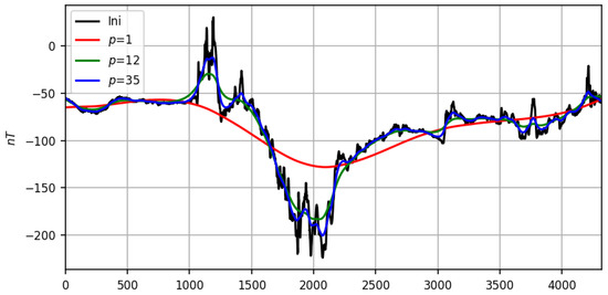
Figure 3.
Results of smoothing on a real recording (black line) at different scales p: (red line), (green line) and (blue line).
Figure 3 shows the performance of the regression smoothing on the real magnetic storm record in the same p-scale parameters as in Figure 2 for the synthetic one. The above figures confirm the convergence proved in Appendix A.1 to the record f of its regression smoothing at .
3. Trend Measure: Preliminary Solution to the Trend Problem
The assumption that a researcher looking at a record f can determine its trend at any node is central to the researcher’s trend logic. Based on it, we construct its implementation using a fuzzy trend measure.
The researcher’s view of the record f is formalized by its regression smoothing based on the proximity (localization) measure on T chosen by the researcher. Next, the researcher is not interested in the smoothing itself, but in the result of its differentiation by the operator : (4). The value of is called the elementary dynamics of the entry f at node t based on the localization of . Their totality, that is, the image , serves as the basis for constructing a fuzzy trend measure . The value in the fuzzy scale expresses the degree of confidence of the researcher (the measure of their reason) to consider the trend of the record f at node t to be positive.
It is constructed as follows: the researcher gives the weight to the elementary dynamics at node . The argument for a positive trend f at node t is all positive dynamics , and against, all negative dynamics with their weights.
The measure of trend is considered the ratio of the sum of the weights of positive dynamics (the argument “for” the positive trend f at node t) to the total sum of weights:
If , then the total argument of the weights of increasing dynamics is greater than the total argument of the weights of decreasing dynamics; therefore, the researcher considers node t to be positive according to the trend for f, and the degree of conditionality of its solution is .
Similarly, if , then node t is considered negative according to the trend for f with a base of and neutral in the case of equality .
Let us summarize the intermediate result: based on the measure , the answer to the first question formulated in the introduction was obtained: “What is a trend at a point?”.
Next, partitioning into positive, negative, and trend-neutral nodes
allows one to simultaneously answer the following two questions of the trend problem: “Which fragments of the record should be considered unconditionally trendy?” and “How do these add up to overall final trends?”
The fact is that in real conditions, there are very few neutral trends from , or none at all. Therefore, it seems natural to consider segments of the record f entirely consisting of positive and neutral (negative and neutral) nodes, respectively, as positive and negative trends () for f: (), a set of nodes without gaps in ().
Definition 4.
We denote an arbitrary trend by : . Trends replace each other and can intersect only at neutral nodes, forming an almost disjunct covering T, which we denote as .
We call the partition a preliminary solution to the trend problem for recording f based on the proximity measure . An explanation of its preliminary nature is given below, but now, we note that strongly depending on , in the case , turns out to be very effective and gives good results at different scales p on difficult real recordings with, in our opinion, a large radius review r. It was this circumstance that served as the reason for writing this work.
The proof is presented in the form of a complete display of the solution to trends : record smoothing trend measure with a partition applied to it → partition on smoothing partitioning into records f. The obvious presence of scale p requires additional effort. Continuing (4) for and omitting the viewing radius r, we introduce the following notation:
- smoothing ,
- elementary dynamics ,
- trend measure ,
- partition .
In order not to confuse the trend measure with the trend segments obtained on its basis, in the latter, we agree to indicate the dependence on the scale p in the form of an argument:
- ,
- .
In Figure 4, Figure 5 and Figure 6, the complete scenario for solving is given for a smooth function on three scales, and for a real record on two scales in Figure 7 and Figure 8.
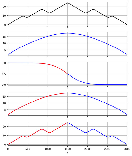
Figure 4.
Preliminary solution of the problem of trends on a smooth record on a scale . Red lines are positive trends, blue lines are negative ones. (a) Original record f. (b) Regression smoothing . (c) Measure of trend with red–blue partition . (d) Partition on smoothing . (e) Partitioning into records f.
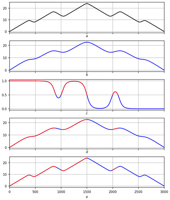
Figure 5.
Preliminary solution of the problem of trends on a smooth record on a scale . Red lines are positive trends, blue lines are negative ones. (a) Original record f. (b) Regression smoothing . (c) Measure of trend with red–blue partition . (d) Partition on smoothing . (e) Partitioning into records f.
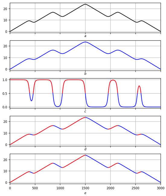
Figure 6.
Preliminary solution of the problem of trends on a smooth record on a scale . Red lines are positive trends, blue lines are negative ones. (a) Original record f. (b) Regression smoothing . (c) Measure of trend with red–blue partition . (d) Partition on smoothing . (e) Partitioning into records f.
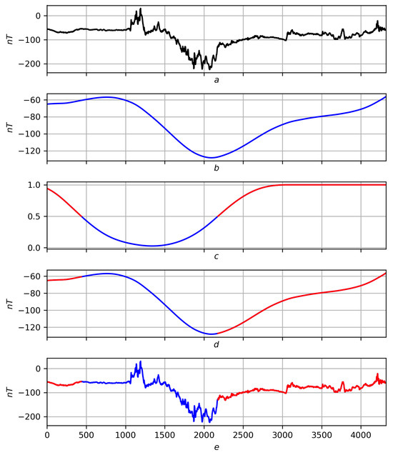
Figure 7.
Preliminary solution of the problem of trends on a real record on a scale . Red lines are positive trends, blue lines are negative ones. (a) Original record f. (b) Regression smoothing . (c) Measure of trend with red–blue partition . (d) Partition on smoothing . (e) Partitioning into records f.
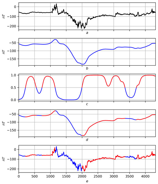
Figure 8.
Preliminary solution of the problem of trends on a real record on a scale . Red lines are positive trends, blue lines are negative ones. (a) Original record f. (b) Regression smoothing . (c) Measure of trend with red–blue partition . (d) Partition on smoothing . (e) Partitioning into records f.
The effectiveness of working in difficult real-world conditions is the main criterion in data analysis, a largely empirical discipline. According to the authors, success in the problem of trends based on the measure lies in two reasons: stability and adequacy.
Stability is a general property of the construction of the measure . Figure 9 illustrates this; Figure 9b,c shows the trend solution on a scale for a smooth record and its disturbance, indicated in Figure 9a in black and green, respectively.
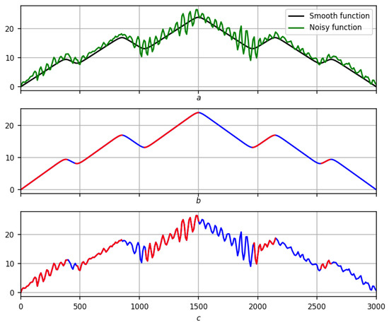
Figure 9.
Stability of the preliminary solution to the trend problem. Red lines are positive trends, blue lines are negative ones. (a) Smooth notation (black) and its disturbance (green). (b) Solution for the smooth recording. (c) Solution to its disturbance.
Adequacy: Trends obtained on the basis of the measure are consistent with the “p” scale: there are no small dynamics in modulus p on smoothing among them. As noted above, it was precisely this circumstance that served as the reason for this work. The explanation of adequacy at the moment is semiempirical: according to the apologetics of regression differential calculus given at the beginning of the work and Appendix A.1, regression derivatives and values inherit the fundamental properties of linear regression, and the measure of trend very naturally depends on them. Therefore, if the effect for trends through regression derivatives exists, then it must necessarily manifest itself through the trend measure. This is illustrated in Figure 10, whose detailed story is given below.
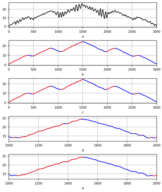
Figure 10.
Adequacy of the preliminary solution to the trend problem. Red lines are positive trends, blue lines are negative ones. (a) Initial recording. (b) Mathematical solution to the trend problem. (c) Preliminary solution to the trend problem. (d) Mathematical solution to the trend problem (fragment). (e) Preliminary solution to the trend problem (fragment).
The stability and adequacy of the solution to the trend problem made it possible to answer the second and third questions relatively simply, i.e., construct final (currently) versions of trend sections of record f at scale p.
This does not always happen. The traditional solution to the trend problem based on smoothing, for example, polynomial, uses a standard mathematical understanding of trends: trends in a record are considered to be mathematical trends in its smoothing. In this solution, the problem of small dynamics remains: on the one hand, smoothing must sufficiently scan the record, on the other hand, the stochastic nature of the record leads to the appearance of small dynamics in the smoothing (short segments of increase/decrease), which a mathematical understanding of the trend in smoothing will highlight as separate trends on the recording.
Let us turn to Figure 10: the classic solution to trends for recording f based on smoothing is shown in Figure 10b, and the solution currently proposed by the authors is in Figure 10c. Selected fragment in Figure 10d,e illustrates the above and shows a greater stability of the solution compared to the classical one. The solution is also better in comparison with the previous solution of the authors, where the trend was obtained in several stages and for this, it was necessary to solve the difficult problem of combining fragments of the f record into a single trend.
However, the solution , despite all the advantages mentioned above, has some inaccuracy that does not allow it to be considered the final solution to the trend problem (Figure 11). To do this, we need a measure of extremity that eliminates the inaccuracy in the solution and adds stability and adequacy to it.
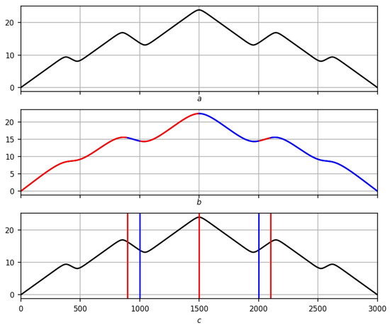
Figure 11.
Partition inaccuracy . (a) Original record. (b) Preliminarily solving the trend problem on a scale . (c) Extrema partition (highs are red, lows are blue, black is the original record).
4. Extremum Measure: The Final Solution to the Trend Problem
In the trend problem, there is one last question about extrema. Of course, the first answer to this question is similar to the classical one: extrema are the boundaries between opposite trends in . On this path, the problem of their existence arises: as noted above, there are few or no neutral nodes from (namely, the extrema should lie within them) due to the stochasticity of f and discreteness of T. The second option, the most natural of the nonempty ones, is as follows: if the positive trend is replaced by a negative , then the maximum should be considered the choice from the end and the beginning , where the entry f is maximum, and, conversely, if the negative trend is replaced by a positive , then the minimum should be considered the choice from the end and the beginning , where the entry f is minimal.
But even after this, some problems remain: the global nature of the trend measure makes the partition stable and quite satisfactory (at least in the case ) on the one hand, and on the other hand, it entails some inaccuracy.
We construct a fuzzy extremum measure , similar to the trend measure : the value in the fuzzy scale of the segment expresses the degree of confidence of the researcher (the measure of their basis) to consider node t the maximum for the function f. Together, the measures and solve the problem of trends: they finally determine the trends and extrema of the record f.
The construction of the measure begins in the same way as the measure : the researcher gives the elementary dynamics at node the weight . If node lies to the left of t (), then the weight speaks in favor of a maximum at t for f with (climbing an imaginary mountain with a peak at t), and against, all with . To the right of t (), everything is the other way around: the weights with (descent from an imaginary mountain with a top at t), and against, all with . The measure of the extremum is considered the sum of the pros to the total sum of weights:
By analogy with the partition , we introduce and denote by the partition by alternating segments obtained by switching : , (Figure 12, Figure 13, Figure 14, Figure 15 and Figure 16). denotes the segment of this partition containing node t.
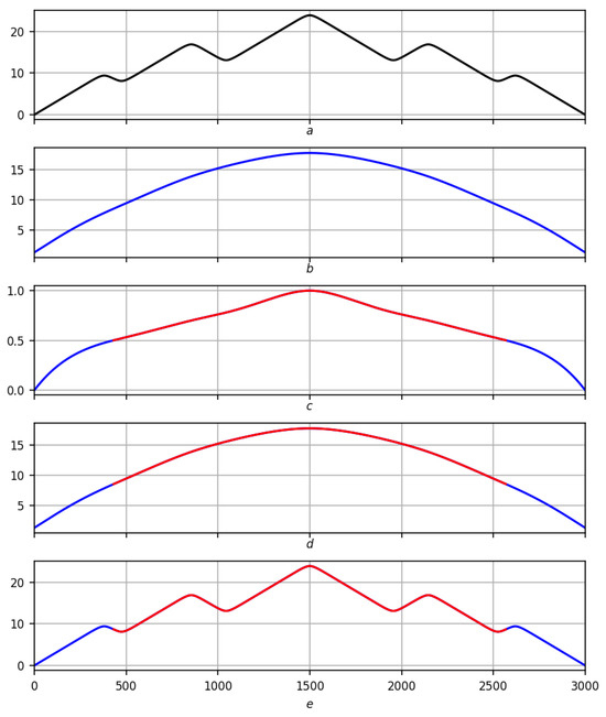
Figure 12.
Partition of on a smooth record on a scale . Red lines are positive trends, blue lines are negative ones. (a) Original record f. (b) Regression smoothing . (c) Measure of extremum with red–blue partition . (d) Partition of on smoothing . (e) Partition of into records f.
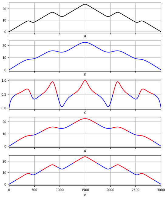
Figure 13.
Partition of on a smooth record on a scale . Red lines are positive trends, blue lines are negative ones. (a) Original record f. (b) Regression smoothing . (c) Measure of extremum with red–blue partition . (d) Partition of on smoothing . (e) Partition of into records f.
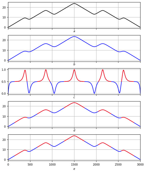
Figure 14.
Partition of on a smooth record on a scale . Red lines are positive trends, blue lines are negative ones. (a) Original record f. (b) Regression smoothing . (c) Measure of extremum with red–blue partition . (d) Partition of on smoothing . (e) Partition of into records f.
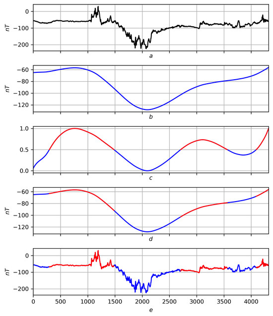
Figure 15.
Partition of on a real record on a scale . Red lines are positive trends, blue lines are negative ones. (a) Original record f. (b) Regression smoothing . (c) Measure of extremum with red–blue partition . (d) Partition of on smoothing . (e) Partition of into records f.
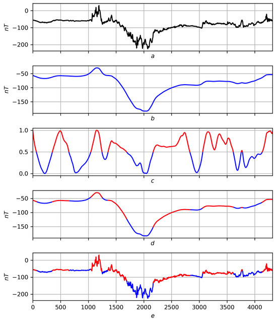
Figure 16.
Partition of on a real record on a scale . Red lines are positive trends, blue lines are negative ones. (a) Original record f. (b) Regression smoothing . (c) Measure of extremum with red–blue partition . (d) Partition of on smoothing . (e) Partition of into records f.
The scheme for displaying the partition is exactly the same as for the partition : record smoothing extremum measure with the partition applied to it → partition on smoothing partition on records f. Taking into account the notations and , in Figure 12, Figure 13 and Figure 14, the full scenario is shown for a smooth function on three scales , and in Figure 15 and Figure 16, for a real recording on a scale .
Let be the version of the maximum obtained above based on . Let us say that it allows a correction if , and the correction itself consists in the transition of to the nearest maximum of the measure on the segment . Similarly, if is a version of the minimum obtained above on the basis of , then it allows a correction if , and the correction itself consists in the transition of to the nearest minimum of the measure on the segment . Extrema based on the measure that do not allow corrections are preserved. This can happen in two situations.
- First, the extremum e is already in the correct position ↔ no correction is needed (it is zero); this happens often, for example, for , and confirms the high efficiency of the measure , as well as solving the problem of trends on its basis.
- Second, the extremum e is not consistent with the measure : or . This means that the measure at the extremum e shows the opposite of its essence: the maximum seems to the researcher to lie in the lowlands, and the minimum on the hills.Let us look at this in more detail, assuming that the maximum is the extremum. Let , be the arguments for (against) the maximum of f in to the left of it; in notation (5) and (6),Similarly, we define arguments , for (against) the maximum of f in to the right of it:In , there is an equilibriumIt allows us to conclude that one-sided extremalities are equivalent for : is the left maximum for —the maximum on the right for f.Further, it follows that .Hence, if the maximum does not allow any correction due to an inconsistency with the measure of extremity (), then is not a maximum on any side. It is probably possible to construct an artificial example of this situation; however, the authors have never encountered this on real recordings. They are calm about the possible appearance of this kind of extrema, since they consider them unstable and, with increasing scale p, either disappearing or turning into normal extrema.
- Third, the extremum e can be consistent with the extremum measure but not unique on the segment . In this case, its trace will necessarily be an extremum that does not allow any correction for the second reason.
Let us summarize: the extremes obtained after correction are considered final, and the segments between them are considered the final trends of the f record. Let us retain their previous designations e, , , noting that after correction, they are the result of the joint activity of the measures and (Figure 17).
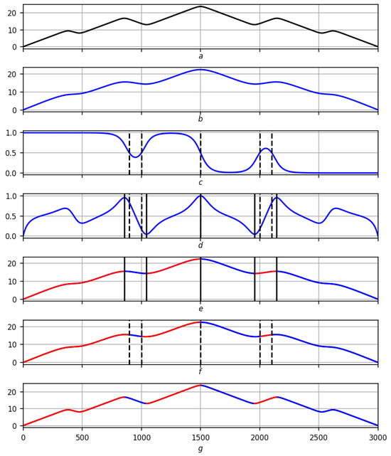
Figure 17.
The final solution of trends for a smooth record on a scale . Red lines are positive trends, blue lines are negative ones. (a) Original record f. (b) Smoothing . (c) Dashed extrema of a preliminary nature on the trend measure . (d) Dashed extrema of a preliminary nature on the trend measure and their solid corrections. (e) Final solution of trends using smoothing . (f) Preliminary solution of trends using smoothing . (g) Final solution of trends on record f.
The correction of extrema for a smooth recording is shown in Figure 17, and for a real recording, in Figure 18, according to the scheme: recording smoothing trend measure with preliminary extrema in strokes → extrema measure with preliminary extrema in strokes and their continuous correction → final solution to the trend problem on smoothing preliminary solution to the trend problem for comparison on smoothing final solution to the trend problem on record f.
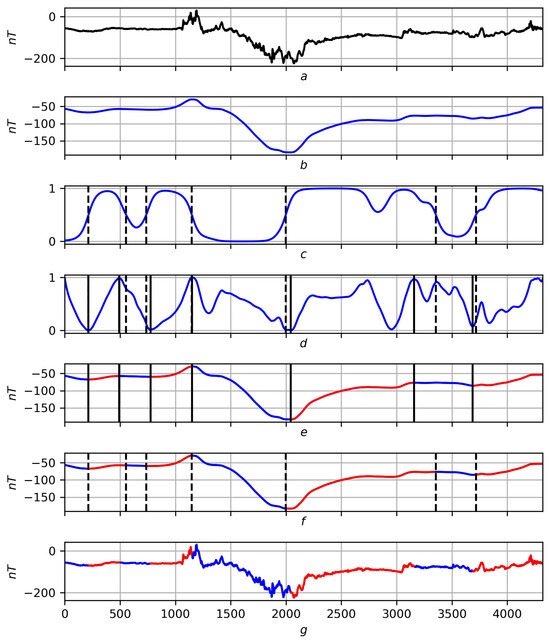
Figure 18.
The final solution of trends for a real record on a scale . Red lines are positive trends, blue lines are negative ones. (a) Original record f. (b) Smoothing . (c) Dashed extrema of a preliminary nature on the trend measure . (d) Dashed extrema of a preliminary nature on the trend measure and their solid corrections. (e) Final solution of trends using smoothing . (f) Preliminary solution of trends using smoothing . (g) Final solution of trends on record f.
5. Various Scales
As mentioned above, there are two dynamic scenarios for tending to node t from the position of the family : the first is for a fixed , the second is for a fixed . In this article, the authors chose the second path, considering that the behavior of , for a large radius gives a more objective dynamic picture of localization at t, since a large number of nodes take a nontrivial part in it (see Definition 1 and the text after Figure 1).
The stability and adequacy of the solution to the problem of trends , the convergence of smoothings to f as , established in Appendix A.1, give reason to believe that a simultaneous analysis of partitions , measures and for different p’s can be useful and allow us to gain knowledge about f at a new level.
The scale parameter p is assumed to be from some discrete uniform segment ; , . The initial scale is usually equal to zero, and the final scale plays the role of infinity . The choice of P is up to the researcher.
The parametric families and , like the wavelet spectrum, characterize the trendiness and extremity of f on a two-dimensional grid at different nodes and scales. Let us use them to determine the hierarchy of extrema on f. The very ability to see the hierarchy of extremes suggests a different scale of the researcher’s view of the record. First, one looks at the recording from the greatest height ↔ at the largest scale. Then, it gradually descends lower, making the viewing scale smaller. Along this path, extrema appear, forming chains. The latter express the migration dependence of the extremum on the scale and generate a hierarchy of extrema: the earlier the chains appear, the more significant the corresponding extremum for the record f.
What was said above according to the scheme “record different-scale partitioning migration of extrema to hierarchy of extrema on record f″ is illustrated for a noisy smooth record in Figure 19, and for a real recording in Figure 20.
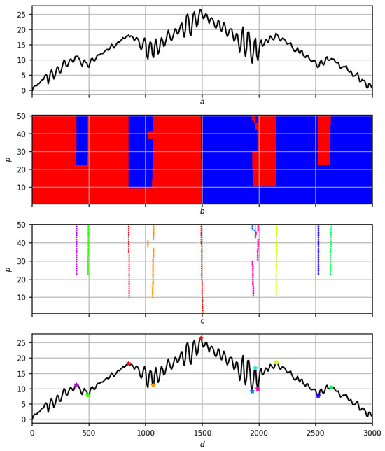
Figure 19.
Multiscale solution of the trend problem on a synthetic record. (a) Original entry f. (b) Partition . Red areas are positive trends, blue areas are negative ones. (c) Migration of extrema to . Different colors correspond to different extrema. (d) Hierarchy of extrema on record f. Asterisks in different colors correspond to extrema on a scale .
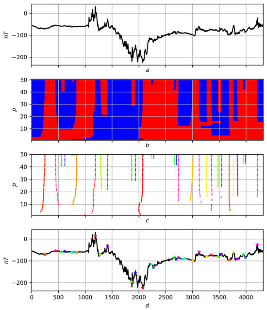
Figure 20.
Multiscale solution of the trend problem on a real record. (a) Original entry f. (b) Partition . Red areas are positive trends, blue areas are negative ones. (c) Migration of extrema to . Different colors correspond to different extrema. (d) Hierarchy of extrema on record f. Asterisks in different colors correspond to extrema on a scale .
Definition 5.
Let be a segment in the final solution of trends at level , which contains the extremum . Let us call the migration : the same oriented end of the segment .
The maximal chains are migration scenarios of the extremum on the grid for record f. For any extremum , let denote the chain passing through it. Note that the extremum can be internal in it: .
Definition 6.
The weight of extremum e is the exponent of the chain containing it.
Next, we take the last level of the scale and all its extrema for f: . Let us order by weights: ; thus, the most fundamental for f is the extremum with the minimum weight.
The identification of trends using trend and extremum measures is stable, and therefore, a multiscale analysis based on these measures is stable and informative. The algorithm for migrating extrema (constructing their chains) proposed in this work is effective only if the quality of their determination is high. The classical approach to trends based on smoothing, for example, polynomial, and using a standard mathematical understanding of trends, is unstable and is not suitable for such an algorithm: a continuation of a really important extremum at one scale level can become a weak (unreasonable) extremum at the next level, which will lead to a migration (chain) of extrema in the wrong direction. As confirmation of what was said earlier, Figure 21 and Figure 22 present a different-scale solution of trends based on a strict mathematical relationship to them for the same records f and on the same scales p as the solutions in Figure 19 and Figure 20. Omitting the details of their comparison, let us pay attention only to the narrow red wedge in Figure 21 slightly to the right of . It is associated with the appearance of unreasonable highs of high rank, while in fact, there should be only one significant minimum, and it is this one that is shown in Figure 19d, and the corresponding chain of migrations is shown in yellow in Figure 19c.
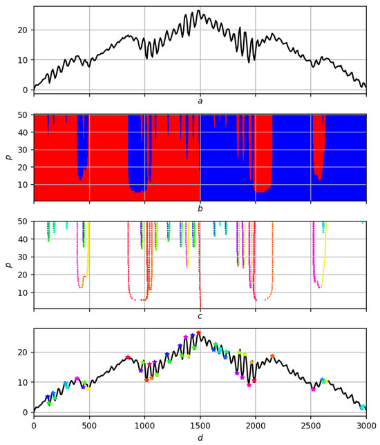
Figure 21.
Multiscale rigorous mathematical solution to the problem of trends on a synthetic record. (a) Original record f. (b) Partition . Red areas are positive trends, blue areas are negative ones. (c) Migration of extrema to . Different colors correspond to different extrema. (d) Hierarchy of extrema on record f. Asterisks in different colors correspond to extrema on a scale .
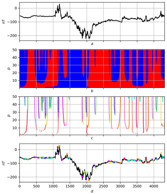
Figure 22.
Multiscale rigorous mathematical solution to the problem of trends on a real record. (a) Original record f. (b) Partition . Red areas are positive trends, blue areas are negative ones. (c) Migration of extrema to . Different colors correspond to different extrema. (d) Hierarchy of extrema on record f. Asterisks in different colors correspond to extrema on a scale .
Note that replacing by and by leads to another dynamic implementation of the above scenario with partitioning by measures and .
6. Trends and Fuzzy Logic
The measures and make it possible to use fuzzy logic in a further study of the record f. The authors plan this in the future, and in this work, we provide two announcements of our research.
- In addition to the measures and , we take into consideration their fuzzy negations and . According to (5) and (6), the measures and are responsible for the increase and maximum of f; therefore, their negations and are responsible for the decrease and minimum of f, respectively. Let us denote their fuzzy disjunction by :We display the manifestation of the measure on the record f in a color scale (Figure 23):
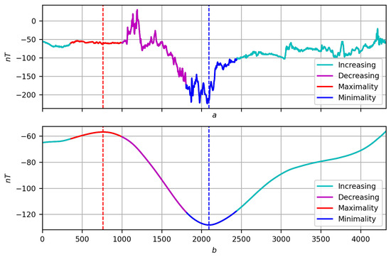 Figure 23. Coding a record by measure . (a) original record f. (b) Its smoothing at with the manifestation of the measure .
- Cyan ↔ manifestation through an increase: ;
- Violet ↔ manifestation through a decrease: ;
- Red ↔ manifestation through a maximum: ;
- Blue ↔ manifestation through minimality: .
Such an encoding of the record by the measure , together with the final solution to the problem of trends for f in the form of a partition , allows us to move further in understanding the behavior of the record through trends.A few first observations: to be specific, the trend is . In the regular case, the increasing trend is a sequential alternation of blue, green and red sections (minimality, growth and maximum). Similarly, a decreasing trend will be an alternation of red, lilac and blue sections (maximum, decrease and minimum). The relationships between the parts indicate both the nature of the extrema (trend boundaries) and the trend itself: the relatively larger the central part, the more singular the extrema, and the more pronounced the trend (Figure 24, , increasing trend containing node 3000 and decreasing trend containing node 3500).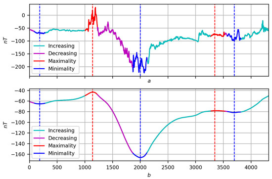 Figure 24. Coding a record by measure : (a) original record f; (b) its smoothing at with the manifestation of the measure .In addition, red or blue inclusions may appear in the central phase: they are outliers in the trend and indicate its stochastic nature (Figure 25, , increasing trend containing node 3000).
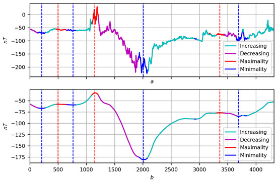 Figure 25. Coding a record by measure : (a) original record f; (b) its smoothing at with the manifestation of the measure .
 - Considering Boolean logic to be part of fuzzy logic, we present a second direction of further research related to it. It concerns the dynamic correlation of records f and g on T in the form of a fuzzy measure . It is constructed similarly to the measures and : the researcher selects a node t and a point of view on T, then each joint elementary dynamics is assigned weight . The argument for the correlation of f and g at t are all equally oriented elementary dynamics, , and against, oppositely oriented elementary dynamics, , with its weights. The correlation measure is considered the ratio of the sums of weights “for” to the total sum of weightsFuzzy negation is a measure of anticorrelation (multidirectionality) of records f and g. The correlation of functions f (Figure 26a) and g (Figure 26b) for proximity on three scales is shown in Figure 27, Figure 28 and Figure 29: the areas where () are shown on the regression smoothings and in red and blue, respectively.
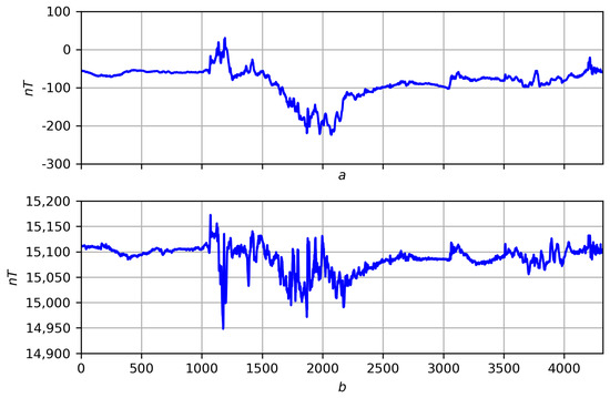 Figure 26. (a) Record f. (b) Record g.
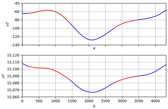 Figure 27. Smoothing functions f and g at with selected areas’ correlations (red is where functions correlate). (a) . (b) .
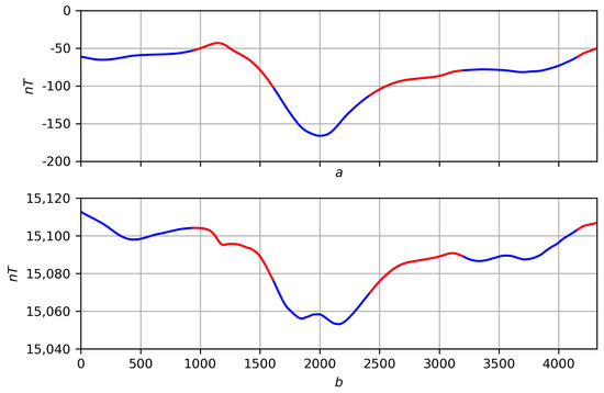 Figure 28. Smoothing functions f and g at with selected areas’ correlations (red is where functions correlate). (a) . (b) .
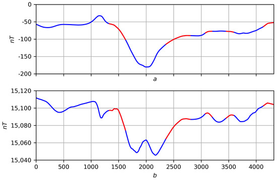 Figure 29. Smoothing functions f and g at with selected areas’ correlations (red is where functions correlate). (a) . (b) .
7. Conclusions
In classical mathematical analysis, the concept of locality is based on a passage to the limit and thus has an infinitesimal character. For this reason, solving the problem of finding trends for piecewise smooth functions is reduced to determining segments of constant sign of the derivative.
In a discrete case, within the framework of DMA, a comparative, fuzzy, multiscale perception of locality is natural and important. It is this perception of locality that is important for analyzing discrete data and understanding the dynamics of the processes that these data express.
Solving the problem of determining trends in discrete time series provides only a preliminary fragmentation of the process. Without identifying the relationship between trends, a deep understanding of the dynamics of the process, which is obtained by constructing a hierarchy of trends and extremes, is impossible.
The theoretical justification of the regression approach to differentiation presented in the work allows, firstly, to give an answer to the question: “What is discrete differentiation”, and secondly, outlines a path for solving the problem of trends at different scales within the framework of the classical approach. It consists in transferring to the continuous case the discrete solution of the trend problem proposed in this work based on measures of trend and extremum by replacing the sum in constructions (5) and (6) with an integral. The efficiency of the discrete solution allows us to hope for success in the continuous case.
About future plans for our research announced in Section 6, we add the following
- A comparative analysis of the solution to the trend problem based on the scale parameter p at a fixed viewing radius with the solution to the trend problem based on the viewing radius r at a fixed scale parameter .
- The trend measures and are very convenient for comparing records f and on scales p and : such a comparison can be any functional distance between fuzzy measures and on the general domain of their definition T. The fuzzy weight of the comparison depends on the researcher. The general conclusion for the set will give a final comparison of a new type between records f and , which is a measure of similarity that can serve as the basis for clustering on records.
- The last direction of further research by the authors, similar to the study of wavelet spectra, is related to the migration of extrema [18,32,33]. It involves two stages: the construction of chains of migration of extrema and their subsequent multifractal analysis (Gibbs sums, scaling exponent, Hölder index). The stage of constructing chains of migration of extremes is described in the proposed article.
In conclusion, we note the following. Regression motives in the analysis of discrete series are present, in particular, in the form of F-transformations (more precisely, -transformations for differentiating a series). Following Zadeh’s principle of incompatibility, they are focused on data analysis for the purpose of decision making. Thus, F-transformations during localization do not deal with the entire family of proximity measures but only with a certain sample , where to effectively simplify calculations [34].
Author Contributions
Conceptualization and original draft preparation, S.A. and D.K.; conceptualization, methodology, review and editing and validation, S.B. and B.D.; material preparation, formal analysis, data curation and algorithm development, S.B. and M.D. All authors contributed to the study conception and design. All authors have read and agreed to the published version of the manuscript.
Funding
This work was conducted in the framework of budgetary funding of the Geophysical Center of RAS, adopted by the Ministry of Science and Higher Education of the Russian Federation (grant number 075-01349-23-00).
Data Availability Statement
No new data were created or analyzed in this study. Data sharing is not applicable to this article.
Conflicts of Interest
The authors declare no conflicts of interest.
Appendix A
Appendix A.1
For the proximity measure on T and its nodes , ; , by , we denote the fraction . For each i, the set is a probability distribution on T: .
Let us denote by the functional of the mathematical expectation relative to this distribution on : , and use it to express the regression value :
where is the series , and is the series .
We are interested in the convergence of as . To achieve this, we require the measure to satisfy two conditions: symmetry and nontrivial strict monotonicity
Let us put . Then, , and for , . Let us consider node internal in T: ; then, due to the conditions on , in the distribution , for any , there are three main actors: and , which we denote by .
Let us reveal the uncertainty of the relation in (A1) by expanding the numerator and denominator modulo :
Numerator:
Denominator:
Thus, as , the fraction tends to zero, and the regression values tends to .
Appendix A.2
The regression approach to derivatives continues into higher dimensions.
Let be a function on the segment having on it continuous derivatives , up to and including order . Under these assumptions, the McLaren decomposition of nth order takes place for :
where is the remainder term in Lagrange form
Let us denote by the Taylor polynomial for [31,35,36,37,38], so that
We fix . Let us denote by the projection of the restriction onto the th subspace of polynomials of degree in the space : is nth order quadratic regression of f on .
Statement A1.
.
The proof follows from the tendency to zero as of the regression .
For simplicity of presentation, let us temporarily omit the dependence on in the coefficients of the polynomials, setting . The regression functional is the distance from to the polynomial in the space :
and the set gives its minimum.
The following equations arise
and the integral
Therefore, the matrix of system (A4) has the form
A nontrivial contribution to the determinant of is made only by even strategies , going along M from left to right: strategy is even ↔ the sum is even in j.
If is an even strategy, then the product of its corresponding matrix elements satisfies the equality
where .
Because of
then
Thus,
where are even strategies and is the signature of the permutation .
The alternative sum K in (A6) is necessarily nontrivial. This is a consequence of Euclidean geometry and linear algebra: the projection in the space onto any of its subspaces always exists and is unique, which, in turn, is equivalent to the nontriviality of . Thus, the order of smallness of the determinant as is equal to .
The next step is to analyze the determinants of the auxiliary matrices of system (A4), obtained from the main M by replacing the th column with a column of free terms:
A nontrivial contribution to is also made only by even strategies: such must necessarily be even for , but always , and therefore, the sum is also even.
Let be any even strategy; then, the product associated with it in is equal to
The determinant is an alternative sum of the products and therefore is and also relative to . The equality completes the proof.
References
- Tanaka, H.; Uejima, S.; Asai, K. Linear regression analysis with fuzzy model. IEEE Trans. Syst. Man Cybern. 1982, 12, 903–907. [Google Scholar]
- Kacprzyk, J.; Wilbik, A.; Zadrożny, S. Linguistic summarization of time series by using the choquet integral. In Lecture Notes in Computer Science; Springer: Berlin/Heidelberg, Germany, 2007; pp. 284–294. [Google Scholar]
- Pedrycz, W.; Smith, M.H. Granular correlation analysis in data mining. In Proceedings of the UZZ-IEEE’99, 1999 IEEE International Fuzzy Systems, Conference Proceedings (Cat. No.99CH36315), Seoul, Republic of Korea, 22–25 August 1999. [Google Scholar]
- Batyrshin, I.Z.; Nedosekin, A.O.; Stetsko, A.A. Fuzzy Hybrid Systems. Theory and Practice; Fizmatlit: Moscow, Russia, 2007. [Google Scholar]
- Yarushkina, N.G. Fundamentals of the Theory of Fuzzy and Hybrid Systems; Finance and Statistics: Moscow, Russia, 2004. [Google Scholar]
- Kovalev, S.M. Hybrid fuzzy-temporal models of time series in problems of analysis and identification of weakly formalized processes. In Integrated Models and Soft Computing in Artificial Intelligence, Proceedings of the IVth International Scientific and Practical Conference, Kolomna, Russia, 28–30 May 2007; Fizmatlit: Moscow, Russia, 2007; Volume 1, pp. 26–41. [Google Scholar]
- Yarushkina, N.G.; Yunusov, T.R.; Afanasyeva, T.V. Terminal-server traffic modeling based on fuzzy time series trend analysis. Softw. Prod. Syst. 2007, 4, 15–19. [Google Scholar]
- Shumway, R.H.; Stoffer, D.S. Time Series Analysis and Its Applications; Springer International Publishing: Berlin/Heidelberg, Germany, 2017. [Google Scholar]
- Brockwell, P.J.; Davis, R.A. Introduction to Time Series and Forecasting; Springer International Publishing: Berlin/Heidelberg, Germany, 2016. [Google Scholar]
- Brockwell, P.J.; Davis, R.A. Time Series: Theory and Methods; Springer: New York, NY, USA, 1987. [Google Scholar]
- Hyndman, R.J.; Athanasopoulos, G. Forecasting: Principles and Practice; OTexts: Melbourne, Australia, 2018. [Google Scholar]
- Agayan, S.M.; Kamaev, D.A.; Bogoutdinov, S.R.; Aleksanyan, A.O.; Dzeranov, B.V. Time series analysis by fuzzy logic methods. Algorithms 2023, 16, 238. [Google Scholar] [CrossRef]
- Montgomery, D.C.; Jennings, C.L.; Kulahci, M. Introduction to Time Series Analysis and Forecasting, 2nd ed.; Wiley: Hoboken, NJ, USA, 2015. [Google Scholar]
- Cryer, J.D.; Chan, K.-S. Time Series Analysis; Springer: New York, NY, USA, 2008. [Google Scholar]
- Tsay, R.S. Analysis of Financial Time Series; Wiley: Hoboken, NJ, USA, 2005. [Google Scholar]
- Greene, W.H. Econometric Analysis; Prentice Hall: Hoboken, NJ, USA, 2003. [Google Scholar]
- Percival, D.B.; Walden, A.T. Wavelet Methods for Time Series Analysis; Cambridge University Press: Cambridge, UK, 2000. [Google Scholar]
- Mallat, S. A Wavelet Tour of Signal Processing; Elsevier: Amsterdam, The Netherlands, 2009. [Google Scholar]
- Yager, R.R. Fuzzy Sets and Possibility Theory; Radio and communications; Pergamon Press: Oxford, UK, 1986. [Google Scholar]
- Zhu, Q.; Batista, G.; Rakthanmanon, T.; Keogh, E. A novel approximation to dynamic time warping allows anytime clustering of massive time series datasets. In Proceedings of the 2012 SIAM International Conference on Data Mining; Society for Industrial and Applied Mathematics, Anaheim, CA, USA, 26–28 April 2012. [Google Scholar]
- Giusti, R.; Batista, G.E. An empirical comparison of dissimilarity measures for time series classification. In Proceedings of the 2013 Brazilian Conference on Intelligent Systems, Fortaleza, Brazil, 19–24 October 2013; IEEE: Piscataway, NJ, USA, 2013. [Google Scholar]
- Ding, H.; Trajcevski, G.; Scheuermann, P.; Wang, X.; Keogh, E. Querying and mining of time series data: Experimental comparison of representations and distance measures. Proc. VLDB Endow. 2008, 1, 1542–1552. [Google Scholar] [CrossRef]
- Batyrshin, I.; Herrera-Avelar, R.; Sheremetov, L.; Panova, A. Moving approximation transform and local trend associations in time series data bases. In Perception-Based Data Mining and Decision Making in Economics and Finance; Springer: Berlin/Heidelberg, Germany, 2007; pp. 55–83. [Google Scholar]
- Almanza, V.; Batyrshin, I. On trend association analysis of time series of atmospheric pollutants and meteorological variables in mexico city metropolitan area. In Lecture Notes in Computer Science; Springer: Berlin/Heidelberg, Germany, 2011; pp. 95–102. [Google Scholar]
- Agayan, S.M.; Bogoutdinov, S.R.; Dobrovolsky, M.N. Discrete perfect sets and their application in cluster analysis. Cybern. Syst. Anal. 2014, 50, 176–190. [Google Scholar] [CrossRef]
- Agayan, S.; Bogoutdinov, S.; Soloviev, A.; Sidorov, R. The study of time series using the DMA methods and geophysical applications. Data Sci. J. 2016, 15, 16. [Google Scholar] [CrossRef]
- Agayan, S.M.; Bogoutdinov, S.R.; Krasnoperov, R.I. Short introduction into DMA. Russ. J. Earth Sci. 2018, 18, 1–10. [Google Scholar] [CrossRef]
- Agayan, S.M.; Bogoutdinov, S.R.; Krasnoperov, R.I.; Efremova, O.V.; Kamaev, D.A. Fuzzy logic methods in the analysis of tsunami wave dynamics based on sea level data. Pure Appl. Geophys. 2022, 179, 4053–4062. [Google Scholar] [CrossRef]
- Agayan, S.M.; Bogoutdinov, S.R.; Dzeboev, B.A.; Dzeranov, B.V.; Kamaev, D.A.; Osipov, M.O. DPS clustering: New results. Appl. Sci. 2022, 12, 9335. [Google Scholar] [CrossRef]
- Kolmogorov, A.N.; Fomin, S.V. Elements of Function Theory and Functional Analysis; Nauka: Moscow, Russia, 1976. [Google Scholar]
- Fichtenholtz, G.M. Differential and Integral Calculus Course; Nauka: Moscow, Russia, 1969. [Google Scholar]
- Muzy, J.F.; Bacry, E.; Arneodo, A. Wavelets and multifractal formalism for singular signals: Application to turbulence data. Phys. Rev. Lett. 1991, 67, 3515–3518. [Google Scholar] [CrossRef] [PubMed]
- Muzy, J.F.; Bacry, E.; Arneodo, A. Multifractal formalism for fractal signals: The structure-function approach versus the wavelet-transform modulus-maxima method. Phys. Rev. E 1993, 47, 875–884. [Google Scholar] [CrossRef] [PubMed]
- Perfilieva, I.; Daňková, M.; Bede, B. Towards a higher degree f-transform. Fuzzy Sets Syst. 2011, 180, 3–19. [Google Scholar] [CrossRef]
- Rudin, U. Principles of Mathematical Analysis; McGraw-Hill: New York, NY, USA, 1976. [Google Scholar]
- Dieudonne, J. Foundations of Modern Analysis; Academic Press, Inc.: Cambridge, MA, USA, 1969. [Google Scholar]
- Schwartz, L. Analysis; Mir: Moscow, Russia, 1972. [Google Scholar]
- Shilov, G.E. Mathematical Analysis; GIFML: Moscow, Russia, 1961. [Google Scholar]
Disclaimer/Publisher’s Note: The statements, opinions and data contained in all publications are solely those of the individual author(s) and contributor(s) and not of MDPI and/or the editor(s). MDPI and/or the editor(s) disclaim responsibility for any injury to people or property resulting from any ideas, methods, instructions or products referred to in the content. |
© 2024 by the authors. Licensee MDPI, Basel, Switzerland. This article is an open access article distributed under the terms and conditions of the Creative Commons Attribution (CC BY) license (https://creativecommons.org/licenses/by/4.0/).