A Novel Approach to Enhance DIRECT-Type Algorithms for Hyper-Rectangle Identification

Abstract

This paper introduces novel enhancements to the most recent versions of DIRECT-type algorithms, especially when dealing with solutions located at the hyper-rectangle vertices. The BIRECT algorithm encounters difficulties in efficiently sampling points at the boundaries of the feasible region, leading to potential slowdowns in convergence. This issue is particularly pronounced when the optimal solution resides near the boundary. Our research explores diverse approaches, with a primary focus on incorporating a grouping strategy for hyper-rectangles of similar sizes. This categorization into different classes, constrained by a predefined threshold, aims to enhance computational efficiency, particularly involving a substantial number of hyper-rectangles of varying sizes. To further improve the new algorithm’s efficiency, we implemented a mechanism to prevent oversampling and mitigate redundancy in sampling at shared vertices within descendant sub-regions. Comparisons with several DIRECT-type algorithms highlight the promising nature of the proposed algorithms as a global optimization solution. Statistical analyses, including Friedman and Wilcoxon tests, demonstrated the effectiveness of the improvements introduced in this new algorithm.

1. Introduction

In scientific and engineering domains, optimization problems often involve objective functions that can only be obtained through ‘black-box’ methods or simulations, frequently lacking explicit derivative information. In cases of black-box optimization, the necessity to optimize various and increasingly complex problems in practice, where analytic information about the objective function is unavailable, has led to the development of derivative-free global optimization methods (DFGO) [1,2,3,4,5,6]. The absence of derivative information necessitates the use of DFGO methods, specifically designed to optimize functions when derivatives are unavailable or unreliable. These techniques explore the function’s behavior by sampling it at various points in the input space.

This paper addresses a global optimization problem

$$\underset{\mathbf{x}\in D}{min}f\left(\mathbf{x}\right),$$

(1)

that only requires the availability of objective function values and no derivative information; therefore, numerical methods using gradient information cannot be used to solve problem (1). The objective function is assumed to be Lipschitz-continuous with some fixed but unknown Lipschitz constant, and the feasible domain is an n-dimensional hyper-rectangle $D=[\mathbf{l},\mathbf{u}]=\{\mathbf{x}\in {\mathbb{R}}^n:l_j\le x_j\le u_j,j=1,\dots ,n\}$.

Global optimization approaches can be categorized into two main types: deterministic [7,8,9,10,11] and stochastic methods [12,13]. These methods address optimization problem (1) using various domain partition schemes, often involving hyper-rectangles [8,13]. While many DIRECT-type techniques employ hyper-rectangular partitions, other alternative approaches use simplicial partitioning [14,15] (such as DISIMPL-C [16] and DISIMPL-V [17]) or diagonal sampling schemes (see [18,19], such as adaptive diagonal curves (ADC) [20]).

DIRECT-type algorithms, such as the DIRECT (divide rectangles) algorithm [21,22] are the most widely used partitioning-based algorithms for global optimization problems. One of the challenges faced by these algorithms is the selection of potentially optimal hyper-rectangles (POHs: the most promising regions), which can lead to inefficiencies and increased computational costs. In this paper, we provide a comprehensive review of techniques and strategies aimed at reducing the set of selected potential optimal hyper-rectangles in DIRECT-type algorithms. We explore various approaches, including a novel grouping strategy that simplifies the identification of hyper-rectangles in the selection procedure. This strategy consists of rounding or approximating the measurements (sizes) of hyper-rectangles, which are extremely small in size, by grouping them together into classes. This simplification can help in various computational or analytical tasks, making the problem more manageable, without significantly compromising the accuracy of the analysis or optimization process.

Our review highlights the importance of reducing the number of function evaluations, while maintaining the algorithm’s convergence properties. Recent papers [23,24] have provided a clear and a comprehensive overview of techniques aimed at reducing the set of potentially optimal rectangles in DIRECT-type algorithms. They have significantly contributed to the field of derivative-free global optimization and serve as a valuable resource for researchers and practitioners seeking to enhance the efficiency and effectiveness of such algorithms. Various suggested methods are summarized in [4,23,24,25,26].

In the context of optimization methods in engineering mathematics, the size of a hyper-rectangle often incorporates constraints imposed by the engineering problem. These constraints ensure that the optimization process adheres to real-world limitations, such as physical boundaries, safety margins, or resource constraints. For example, in structural engineering, the size of a hyper-rectangle could represent the permissible range for material properties, dimensions, or loads. In engineering optimization, reducing the size of a hyper-rectangle can signify the imposition of stricter constraints. This ensures that the optimized solution adheres to more rigorous requirements, such as safety limits or design specifications.

We also use an additional assumption to improve this version, thus allowing the evaluation of the objective function only once at each vertex of each hyper-rectangle. The objective function values at vertices can be stored in a special vertex database, and then the result is directly retrieved from this database when required. In addition, an update to the modified optimization domain is applied for some test problems, as used in the previous version [27].

In reference to [6,25], the DIRECT algorithm is subject to various strengths and weaknesses. The weaknesses are briefly summarized below. For an in-depth presentation and analysis, please refer to [6,25].

First, DIRECT exhibits a relatively low convergence rate when refining solutions. Second, the exploration around local minima may potentially delay the identification of the global minimum. Third, there are instances where it fails to effectively leverage local trends. Fourth, the algorithm’s performance tends to degrade in higher dimensions. Fifth, additionally, it demonstrates inflexibility in its center-based sampling and partitioning scheme, leading to slow convergence to an optimum on the boundary.

Based on the existing literature, a variety of studies have been conducted on the weaknesses of DIRECT from various perspectives [6]. However, the following potential research gaps remain: The original DIRECT algorithm faces challenges when it comes to sampling points at the edges of the feasible region, which can slow down its convergence, particularly in cases where the best solution is located at the boundary. This limitation is especially pronounced in constrained problems. Recent research [24,28,29] has emphasized the importance of addressing this issue, showing that it is possible to achieve faster convergence by employing strategies that sample points at the vertices of hyper-rectangles, especially when solutions are near the boundary. However, an extension, referencing our approach [30], to handle global optimization problems involving Lipschitz continuous functions subject to linear constraints addresses the limitations of existing techniques, which mainly focus on bound constraints and encounter difficulties when faced with infeasible regions [29]. For DIRECT-type algorithms, this poses a significant challenge, as they must partition these regions to reveal feasible areas, leading to a considerable number of function evaluations being wasted.

Taking these insights into account, we have integrated one of the latest versions of the DIRECT-type algorithm into our approach, a new diagonal partitioning and sampling scheme called BIRECTv (bisection of rectangles with vertices) [27]. In the BIRECTv framework, the objective function is evaluated at specific points within the initial hyper-rectangle. Instead of evaluating the objective function only at the vertices, as done in most DIRECT-type algorithms, BIRECTv samples two points along the main diagonal of the initial hyper-rectangle, located $1/3$ and 1 of the way along the diagonal. This adaptation provides more comprehensive information about the objective function and enhances the exploration of boundary regions, thereby improving the algorithm’s convergence performance in such scenarios. By employing a strategy that samples two points per hyper-rectangle, this partitioning technique reduces the likelihood of the algorithm choosing suboptimal points within a hyper-rectangle containing an optimal solution, (see e.g., [20,24]). This approach offers a notable advantage over center sampling methods, particularly when the majority of solution coordinates fall within specified boundaries. Furthermore, to ensure the reliability and significance of our results, we employed statistical analyses, including Friedman [31] and Wilcoxon [32] tests, to validate the effectiveness of the improvements introduced to this algorithm compared to existing optimization solvers for such problems.

A literature review was conducted to identify the research gaps addressed in this study. The contributions and novelties of this study are summarized as follow:

• Dedicated Vertex Database Integration: This work introduces a new approach by incorporating a dedicated vertex database. The purpose of this strategic embedding is to constrain sampling points within descent sub-regions, effectively mitigating the risk of oversampling. By implementing this vertex database, the algorithm provides more efficient computations, improving both the accuracy and speed of the optimization process.
• Innovative Grouping Strategy for Hyper-Rectangle Identification: A groundbreaking grouping strategy is introduced, specifically designed for the efficient identification of hyper-rectangles in DIRECT-type algorithms. This innovation addresses the challenge of managing and organizing data points in the search space. By taking advantage of this advanced clustering strategy, the algorithm optimizes the hyper-rectangle identification process, resulting in a more rational and powerful exploration of the solution space.
• Performance Enhancement in the BIRECTv Algorithm: This paper outlines the significant improvements made to the BIRECTv algorithm. These developments have a positive and noticeable impact on the overall efficiency of the algorithm. By refining the BIRECTv approach, this research contributes to a more robust and efficient optimization algorithm, with advances in convergence rates and solution quality. The refined BIRECTv algorithm illustrates the practical implications of the suggested contributions in the design of the underlying optimization process.

The remaining sections of this paper are arranged as follows: Section 2 is devoted to an overview of the existing methods for selecting (POHs) in various DIRECT-type approaches. In Section 3.1, a review of the original BIRECT algorithm is provided, while in Section 3.2 a brief description of the new sampling and partitioning scheme called the BIRECTv algorithm is given. In Section 3.3, we incorporate a novel scheme for grouping and selecting potential optimal hyper-rectangles in BIRECT-type algorithms. In Section 4, a numerical investigation and discussion of the results are provided. The algorithmic performance and evaluation metrics are presented in Section 4.3. Additionally, several main statistical methods and techniques, such as Friedman and Wilcoxon tests, are introduced in Section 4.4. In Section 5, the paper’s findings are summarized, and potential directions for future prospects are outlined.

2. Overview of Existing Methods for Selecting (POHs) in Various DIRECT-Type Approaches

This section provides a short discussion on the existing methods used for the selection of POHs in various DIRECT-type approaches.

The field of optimization algorithms has undergone significant advancements, as shown by recent research contributions. The BIRECTv algorithm represents a significant evolution of the BIRECT algorithm, with a particular focus on improving its ability to identify hyper-rectangles. Meanwhile, a new DIRECT-type algorithm specifically designed for hyper-rectangle identification was presented in another research paper, highlighting the importance of rectangles in identifying potentially optimal hyper-rectangles for optimization tasks [33]. In addition, a separate article discussed the improvements made to the modified version of the BIRECT algorithm, called BIRECTv, and focused on hyper-rectangle identification improvements [27]. Another study provided a comprehensive exploration of hyper-rectangle splitting in the DIRECT algorithm, revealing an improved strategy for identifying potentially optimal hyper-rectangles, with the full text offering detailed insights into the algorithmic enhancements [25]. Further contributing to DIRECT optimization, a study proposed a new strategy for selecting potentially optimal hyper-rectangles, thereby enriching our understanding of optimization algorithms [23].Finally, an experimental study highlighted the effectiveness of the well-known derivative-free global search algorithm DIRECT, giving an overview of its performance and its practical benefits in solving optimization problems [34]. Together, these works represent a variety of advances, refining and extending the capabilities of optimization algorithms for hyper-rectangle identification and global search tasks.

Various strategies have been developed to enhance this selection process, resulting in different versions of the algorithm. In the DIRECT-l variant [25,35], the size of a hyper-rectangle is measured using the length of its longest side, which corresponds to the infinity norm. This approach allows DIRECT-l to group more hyper-rectangles with the same measure, resulting in fewer distinct measures. Moreover, in DIRECT-l, only one hyper-rectangle from each group is selected, even if there are multiple POHs in the same group. This reduces the number of divisions within a group. DIRECT-l has been found to perform well for lower-dimensional problems that do not have an excessive number of local and global minima.

The aggressive version of DIRECT [36] takes a different approach by selecting and dividing a hyper-rectangle of every measure in each iteration. While this strategy requires more function evaluations compared to other versions of DIRECT, it may be advantageous for solving more complex problems. The PLOR algorithm [37] (Pareto–Lipschitzian optimization with reduced-set), simplifies the set of POHs to just two: the maximal and the minimal Lipschitz constants. This reduction allows the PLOR approach to be independent of user-defined parameters. It strikes a balance between local and global search during the optimization process by considering only these two extreme cases.

In two-phase globally and locally biased algorithms, the selection procedure during one of the phases operates similarly to the original DIRECT algorithm, considering all hyper-rectangles from the current partition. However, in the second phase, the selection of POHs is constrained based on their measures. Globally-biased versions [17,20] focus on larger subregions, addressing the algorithm’s first weakness, while locally-biased versions [35,38] concentrate on smaller subregions, addressing the second weakness of DIRECT-type algorithms. These adaptations and strategies aim to improve the efficiency and effectiveness of DIRECT-type algorithms in addressing optimization challenges, particularly in scenarios with complex landscapes and varying dimensions [3,29].

The authors in [23] introduced an improved scheme by extending the set of POHs in a new DIRECT-type algorithm called DIRECT-GL algorithm. These enhanced criteria are designed to reduce the computational cost of the algorithm by focusing on the most promising regions of the search space. By implementing improved selection criterion, the algorithm becomes more efficient in identifying regions of interest within the optimization landscape. This leads to a reduction in the number of hyper-rectangles that need to be explored, saving computational resources and time. The enhancements introduced in this work are not limited to a specific type of problem or application. They can be applied to a wide range of optimization scenarios where DIRECT-type algorithms are utilized [24,39,40].

3. From BIRECT to BIRECTv(impr.)

This section provides an overview of the original BIRECT algorithm and its modifications.

3.1. The Original BIRECT

The BIRECT (bisection of rectangles) algorithm, developed in [41], employs a diagonal space-partitioning approach and involves two primary procedures, namely sampling on diagonals and bisection of hyper-rectangles.

In the initialization step, the algorithm begins by evaluating the objective function at two initial points, “lower” $\mathbf{l}=(l_1,\dots ,l_n)={(1/3,\dots ,1/3)}^T$ and “upper” $\mathbf{u}=(u_1,\dots ,u_n)={(2/3,\dots ,2/3)}^T$, positioned along the main diagonal of the normalized domain, considered as the first unit hyper-cube, $\overline{D}={\overline{D}}_0^1=[\overline{\mathbf{l}},\overline{\mathbf{u}}]=\{\overline{\mathbf{x}}\in {\mathbb{R}}^n:0\le \overline{l_j}\le \overline{\mathbf{x}}\le \overline{u_j}\le 1,j=1,\dots ,n\}$. The hyper-cube representing the search space is then divided into a set of smaller hyper-rectangles obeying a specific sampling and partitioning scheme using the following criteria (see Algorithm 1).

3.1.1. Selection Criterion

• At each iteration (kth iteration), starting from the current partition

  $${\mathcal{P}}_k=\{{\overline{D}}_k^i:i\in {\mathbb{I}}_k\},$$

  where ${\mathbb{I}}_k$ is the index set identifying the current partition, a new partition ${\mathcal{P}}_{k+1}$ is created by bisecting a set of POHs from the previous partition.
• The identification of a potentially optimal hyper-rectangle (POH) is based on lower bound estimates of the objective function over each hyper-rectangle, with a fixed rate of change $\tilde{L}>0$ (analogous to a Lipschitz constant).
• A hyper-rectangle ${\overline{D}}_k^j$, $j\in {\mathbb{I}}_k$ is considered potentially optimal if specific inequalities involving $\epsilon$ (a positive constant) and the current best-known function value $f_{\min }$ are satisfied.

  $$\begin{array}{ccc}\hfill min\left\{f\left({\mathbf{l}}^j\right),f\left({\mathbf{u}}^j\right)\right\}-\tilde{L}{\delta }_j^k& \le & min\left\{f\left({\mathbf{l}}^i\right),f\left({\mathbf{u}}^i\right)\right\}-\tilde{L}{\delta }_i^k,\forall i\in {\mathbb{I}}_k\hfill \end{array}$$

  (2)

  $$\begin{array}{ccc}\hfill min\left\{f\left({\mathbf{l}}^j\right),f\left({\mathbf{u}}^j\right)\right\}-\tilde{L}{\delta }_j^k& \le & f_{min}-\epsilon \left|f_{min}\right|,\hfill \end{array}$$

  (3)

  where the measure (distance, size) of the hyper-rectangle is given by

  $${\overline{\delta }}_k^i=\frac{2}{3}\parallel {\overline{\mathbf{b}}}^i-{\overline{\mathbf{a}}}^i\parallel .$$

  (4)

The $\parallel .\parallel$ on the right-hand side of Equation (4), represents the standard Euclidean 2-norm. The measure of a hyper-rectangle is determined using the Euclidean distance from its sampled point along the main diagonal to the farthest vertex, or equivalently, using two-thirds of the length of a diagonal. A hyper-rectangle ${\overline{D}}_k^j$ is potentially optimal if the lower bound for f computed by the left-hand side of (2) is optimal for some fixed rate of change $\tilde{L}$ among the hyper-rectangles of the current partition ${\mathcal{P}}_k$. The second criterion (3) requires that the lower bound of the hyper-rectangle must surpass the current best solution ($f_{min}$). To be precise, it should be less than or equal to $f_{min}-\epsilon \left|f_{min}\right|$. This condition serves as a threshold to prevent the algorithm from expending function evaluations on hyper-rectangles with extremely small bounds that are unlikely to yield significant improvements. The practical choice of $\epsilon$ can vary, in the study [21], favorable outcomes were obtained with $\epsilon$ values ranging from ${10}^{-2}$ to ${10}^{-7}$.

Algorithm 1 Main steps of the BIRECT algorithm

1: $\mathbf{Input}:$ Objective function: f, search-space: D, tolerance: ${ϵ}_{pe}$, the maximal number of function evaluations: $M_{max}$, and the maximal number of iterations: $K_{max}$; 2: $\mathbf{Output}:$ The best objective function value: $f_{min}$, global minimizer: $x_{min}$, and algorithmic performance measures: m, k and $pe$ (if needed); 3: Normalize the search space D to the unit hyper-cube $\overline{D}$; 4: Initialize ${\mathit{l}}^1=(1/3,\dots ,1/3)$ and ${\mathit{u}}^1=(2/3,\dots ,2/3)$, evaluate $f\left({\mathbf{l}}^1\right)$ and $f\left({\mathbf{u}}^1\right)$, and set $f_{min}=min\left\{f\left({\mathbf{l}}^1\right),f\left({\mathbf{u}}^1\right)\right\}$, $x_{min}=\underset{x\in \{{\mathbf{l}}^i,{\mathbf{u}}^i\}}{\mathrm{argmin}}f\left(x\right)$, $m=2$, $k=1$, ${\mathbb{I}}_k=\left\{1\right\}$; 5: while $pe>{\epsilon }_{\mathrm{pe}}$ and $m<{\mathrm{M}}_{max}$ and $k<{\mathrm{K}}_{max}$ do 6:     Identify the index set ${\mathbb{P}}_k\subseteq {\mathbb{I}}_k$ of potentially optimal hyper-rectangles (POHs); 7:     Set ${\mathbb{I}}_k={\mathbb{I}}_k\setminus \left\{{\mathbb{P}}_k\right\}$; 8:     for $i\in {\mathbb{P}}_k$ do 9:         Select the branching variable $\mathbf{br}$ (coordinate index) Equation (5); 10:         Divide ${\overline{D}}^i$ into a two new hyper-rectangles ${\overline{D}}^{m+1}$ and ${\overline{D}}^{m+2}$. Update ${\delta }_{m+1}$ and ${\delta }_{m+2}$; 11:         Create the new sampling points ${\mathit{l}}^{m+1}$ and ${\mathit{u}}^{m+2}$; 12:         Update the partition set: ${\mathcal{P}}_k={\mathcal{P}}_k\setminus {\overline{D}}_k^j\cup {\overline{D}}_k^{m+1}\cup {\overline{D}}_k^{m+2}$; 13:         if $f_{min}^{m+1}\le f_{min}$ or $f_{min}^{m+1}\le f_{min}$ then 14:            Update $f_{min}$ and $x_{min}$; 15:         end if 16:         Update performance measures: k, m and $pe$; 17:     end for 18: end while 19: $\mathbf{Return}:$ $f_{min}$, $x_{min}$ and algorithmic performance measures: m, k and $pe$.

3.1.2. Division and Sampling Criterion

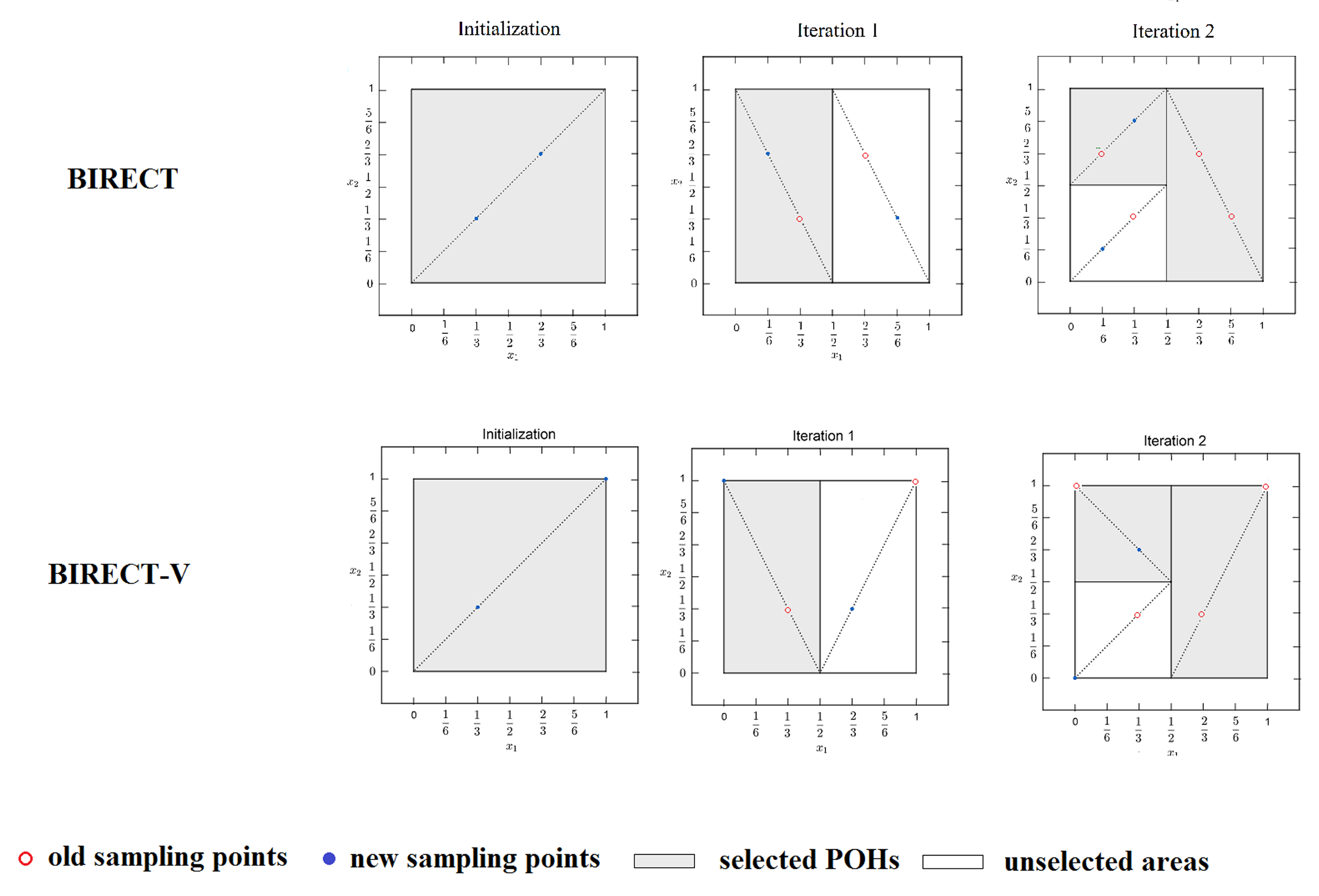
• After the initial partitioning, BIRECT proceeds to future iterations by partitioning POHs and evaluating the objective function $f\left(x\right)$ at new sampling points.
• New sampling points are generated by adding and subtracting a distance equal to half the side length of the branching coordinate from the previous points. This approach allows for the reuse of old sampled points in descendant subregions.
• An important aspect of the algorithm is how the selected hyper-rectangles are divided. For each POH, the set of maximum coordinates (edges) is computed, and the hyper-rectangle is bisected along the coordinate (branching variable $x_{br},$ $1\le br\le n$) with the largest side length ($d_{br}^i$). Starting from the coordinates associated with the smallest index j (in case multiple coordinates are eligible):

$$br=min\left\{\underset{1\le j\le n}{argmax}=\left\{d_j^i=\left|b_j^i-a_j^i\right|\right\}\right\},$$

(5)

and by using the exact bisection [42]. The division is limited to only being performed along the longest coordinate of the hyper-rectangle. This constraint guarantees that, during each iteration, the hyper-rectangles will contract along one dimension. The partitioning process continues until a predefined number of function evaluations has been performed or a stopping criterion is satisfied. The algorithm keeps track of the best (smallest) objective function value $f\left(\overline{\mathbf{x}}\right)$ found over all sampled points in the final partition. The corresponding generated point $\overline{\mathbf{x}}$ at which this value was achieved, provides an approximate solution to the optimization problem. The main steps of the BIRECT algorithm are outlined in Algorithm 1 (see [41] for a detailed pseudo-code).

The BIRECT algorithm is a robust optimization technique that efficiently explores the search space, combines global and local search strategies, and strives to find the optimal or near-optimal solution for multidimensional optimization problems. For a more comprehensive understanding, additional details can be found in the original paper [41].

3.2. Description of the BIRECTv Algorithm

In this subsection, we revert to one of the most recent versions of DIRECT-type algorithms (called BIRECTv) developed in [27]. One effective strategy is to sample points at the vertices of the hyper-rectangles. This approach ensures that points near the boundaries are explored, increasing the chance of finding solutions located there. Sampling at vertices can significantly improve convergence when the optimal solution is at or near the boundary, see [29]. A description of two different partitioning schemes used in DIRECT-type algorithms is shown in Figure 1.

The original DIRECT algorithm primarily focuses on sampling within the interior of the feasible region, which means it may miss exploring points near the boundary. Therefore, it may require a large number of iterations to converge to the optimal solution. This slow convergence is because it relies on subdividing hyper-rectangles within the interior, and it may take many iterations before a hyper-rectangle boundary coincides with the solution. The studies conducted in [3,43] indeed highlighted the significant impact of the limitation in convergence when the optimal solution lies at the boundary of the feasible region. This issue is particularly prevalent in constrained optimization problems, where solutions often lie at the boundary due to the constraints imposed on the variables.

However, a challenge arises when the newly created sampling points coincide with previously evaluated points at shared vertices. This leads to additional evaluations of the objective function, increasing the number of function evaluations per iteration. To address this issue, the paper suggested modifying the original optimization domain to obtain a good approximation of the global solution.

This approach was presented as an alternative to locate solutions that are situated near the boundary. The results of the experiments demonstrated that the proposed modification to the optimization domain positively impacted the performance of the BIRECTv algorithm. It outperformed the original BIRECT algorithm and the two popular DIRECT-type algorithms on the test problems. Additionally, the BIRECTv algorithm showed particular efficacy in solving high-dimensional problems.

3.3. Integration Scheme for Identification of Potentially Optimal Hyper-Rectangles in DIRECT-Based Frameworks

In this section, we introduce an innovative grouping technique that streamlines the hyper-rectangle identification process during selection. This approach involves the rounding or approximation of measurements (sizes) for hyper-rectangles of exceedingly small dimensions. These are then organized into classes, yielding a simplification that enhances the manageability of computational and analytical tasks. Importantly, this simplification does not substantially impact the precision of the analysis or optimization process. The selection of the most promising hyper-rectangles in DIRECT-type algorithms is a crucial aspect of optimization.

Let the partition of ${\overline{D}}_k^i$ at iteration k be defined as

$${\mathcal{P}}_k=\{{\overline{D}}_k^i:i\in {\mathbb{I}}_k\},$$

Let ${\mathbb{I}}_k$ be the set of indices identifying the subsets defining the current partition ${\mathcal{P}}_k$. Let ${\overline{\delta }}_k^i$ be a measure of ${\overline{D}}_k^i$ defined Equation (4)

Let ${\mathbb{I}}_k^i\subseteq {\mathbb{I}}_k$ represent a subset of indices that correspond to elements of ${\mathcal{P}}_k$, with measure ${\delta }_k^i$ having almost the same measure as ${\overline{\delta }}_k^i$ within a certain tolerance (threshold = $\Delta$), ranging from ${10}^{-7}$ to ${10}^{-2}$, i.e., such that $\Delta =\left\{{10}^{-7},{10}^{-6},{10}^{-5},{10}^{-4},{10}^{-3},{10}^{-2}\right\}$.

$$\mathtt{diff}=\left|{\overline{\delta }}_k^i-{\delta }_k^i\right|\le \Delta ,i\in {\mathbb{I}}_k^i.$$

(6)

In Equation (6), the diff on the left-hand side represents the absolute difference between the scalar numerical value ${\overline{\delta }}_k^i$, and an array of numerical values ${\delta }_k^i$. The purpose is to identify POHs. This looks for hyper-rectangles (indexed by I) where the norm value (${\delta }_k^i$) is very close (within the defined tolerance) to the normalized norm value (${\overline{\delta }}_k^i$).

Line 11 is used to reduce the set of POHs. The code filters the hyper-rectangles and selects only those that meet a specific condition, which is having a norm value (${\delta }_k^i$) close to the normalized norm value (${\overline{\delta }}_k^i$) within a tolerance of $0.0001$.

In summary, this line of code helps to focus on potentially more promising hyper-rectangles, discarding those that are not as close to the desired normalized norm value. This is a way to efficiently narrow down the search space and improve the efficiency of the algorithm. An illustrative example for two different tolerance levels is given in Figure 2.

The difference between the tolerance ${10}^{-2}$ and ${10}^{-7}$ lies in the level of precision used when comparing the ${\delta }_k^i$ and ${\overline{\delta }}_k^i$ values used to filter the POHs.

• Tolerance ${10}^{-2}$:
  • A tolerance of ${10}^{-2}$ (0.01) means that the algorithm will consider hyper-rectangles whose ${\delta }_k^i$ and ${\overline{\delta }}_k^i$ values are within 0.01 of each other.
  • This allows for a relatively larger difference between ${\delta }_k^i$ and ${\overline{\delta }}_k^i$, meaning the algorithm will be more lenient in selecting POHs.
  • This might result in a larger set of POHs, including some with relatively larger differences in their norm values.
• Tolerance ${10}^{-7}$:
  • A tolerance of ${10}^{-7}$ (0.0000001) means that the algorithm will consider hyper-rectangles whose ${\delta }_k^i$ and ${\overline{\delta }}_k^i$ values are within $0.0000001$ of each other.
  • This uses a much smaller tolerance, making the algorithm much stricter in selecting POHs.
  • This will result in a smaller set of POHs, only including those with extremely close norm values.

The choice of tolerance depends on the specific problem and the desired level of precision in the algorithm. A larger tolerance may lead to faster execution, but it might also include some hyper-rectangles that are not truly optimal. On the other hand, a smaller tolerance will be more accurate but may require more computational effort to identify the POHs. There is a trade-off between efficiency and precision in the algorithm’s behavior.

Note: The algorithm assumes a zero-based index for the array elements, and the first index found satisfying the condition is returned. If no element satisfies the condition, the algorithm returns −1.

The algorithm essentially performs a linear search through the ${\delta }_k^i$ array and stops as soon as it finds the first element within the specified tolerance level. It is important to choose an appropriate tolerance level depending on the application and the expected values in the array.

Convergence

The existing literature has extensively explored the convergence characteristics of DIRECT-type algorithms (see e.g., [4,20,21,35,41]). These algorithms, including BIRECTv, are often categorized as ‘divide the best’ methods and exhibit a form of convergence known as ‘everywhere dense’. This means they converge at every point within the feasible region. As the algorithm progresses, each explored point becomes an accumulation point, gradually leading to the sampling of points that approach the global solution. The convergence framework of BIRECTv aligns with this established pattern, in the sens of the ‘everywhere-dense’ type of convergence. In addition, the continuity of the objective function in the neighborhood of global minima is a sufficient assumption that guarantees convergence.

4. Results and Discussion

4.1. Implementation

In this section, we provide an overview of the methodology and objectives of our study, which involved benchmarking the new enhanced BIRECTv against the previous version of BIRECTv [27], the original BIRECT [26,41], and other DIRECT-type algorithms on a set of test problems. In our study, the size of the hyper-rectangle in BIRECTv was measured using the same criterion as in the original BIRECT algorithm. In contrast, for DIRECT-l, this corresponds to the infinity norm, allowing it to collect more hyper-rectangles of the same size. This is different from the Euclidean distance measure used in the original DIRECT algorithm. Our implementation used the same set of 54 global optimization test problems from [44]. The Hedar test set is a popular benchmark for testing optimization algorithms, and its problems are described in

Table A1. Key characteristics of the Hedar test problems [44], with modified test problems denoted by a star.

Problem No.	Problem Name	Dimension n	Feasible Region $\mathit{D}=([{\mathit{a}}_{\mathit{j}},{\mathit{b}}_{\mathit{j}}],\mathit{j}=\mathbf{1},\dots ,\mathit{n})$	No. of Local Minima	Optimum ${\mathit{f}}^{\ast }$
$1^{\ast },2^{\ast },3^{\ast }$	Ackley	2, 5, 10	${[-15,35]}^n$	multimodal	0.0
4	Beale	2	${[-4.5,4.5]}^2$	multimodal	0.0
$5^{\ast }$	Bohachevsky 1	2	${[-100,110]}^2$	multimodal	0.0
$6^{\ast }$	Bohachevsky 2	2	${[-100,110]}^2$	multimodal	0.0
$7^{\ast }$	Bohachevsky 3	2	${[-100,110]}^2$	multimodal	0.0
8	Booth	2	${[-10,10]}^2$	unimodal	0.0
9	Branin	2	$[-5,10]\times [10,15]$	3	$0.39789$
10	Colville	4	${[-10,10]}^4$	multimodal	0.0
$11,12,13$	Dixon & Price	2, 5, 10	${[-10,10]}^n$	unimodal	0.0
14	Easom	2	${[-100,100]}^2$	multimodal	$-1.0$
15	Goldstein & Price	2	${[-2,2]}^2$	4	3.0
${16}^{\ast }$	Griewank	2	${[-600,700]}^2$	multimodal	0.0
17	Hartman	3	${[0,1]}^3$	4	$-3.86278$
18	Hartman	6	${[0,1]}^6$	4	$-3.32237$
19	Hump	2	${[-5,5]}^2$	6	$-1.03163$
$20,21,22$	Levy	2, 5, 10	${[-10,10]}^n$	multimodal	0.0
${23}^{\ast }$	Matyas	2	${[-10,15]}^2$	unimodal	0.0
24	Michalewics	2	${[0,\pi ]}^2$	2!	$-1.80130$
25	Michalewics	5	${[0,\pi ]}^5$	5!	$-4.68765$
26	Michalewics	10	${[0,\pi ]}^{10}$	10!	$-9.66015$
27	Perm	4	${[-4,4]}^4$	multimodal	$0.0$
$28,29$	Powell	4, 8	${[-4,5]}^n$	multimodal	$0.0$
30	Power Sum	4	${[0,4]}^4$	multimodal	$0.0$
${31}^{\ast },{32}^{\ast },{33}^{\ast }$	Rastrigin	2, 5, 10	${[-5.12,6.12]}^n$	multimodal	$0.0$
$34,35,36$	Rosenbrock	2, 5, 10	${[-5,10]}^n$	unimodal	$0.0$
$37,38,{39}^{\ast }$	Schwefel	2, 5, 10	${[-500,500]}^n$	unimodal	$0.0$
40	Shekel, $m=5$	4	${[0,10]}^4$	5	$-10.15320$
41	Shekel, $m=7$	4	${[0,10]}^4$	7	$-10.40294$
42	Shekel, $m=10$	4	${[0,10]}^4$	10	$-10.53641$
43	Shubert	2	${[-10,10]}^2$	760	$-186.73091$
${44}^{\ast },{45}^{\ast },{46}^{\ast }$	Sphere	2, 5, 10	${[-5.12,6.12]}^n$	multimodal	$0.0$
${47}^{\ast },{48}^{\ast },{49}^{\ast }$	Sum squares	2, 5, 10	${[-10,15]}^n$	unimodal	$0.0$
50	Trid	6	${[-36,36]}^6$	multimodal	$-50.0$
51	Trid	10	${[-100,100]}^{10}$	multimodal	$-210.0$
${52}^{\ast },{53}^{\ast },{54}^{\ast }$	Zakharov	2, 5, 10	${[-5,11]}^n$	multimodal	$0.0$

, including attributes like problem number, problem name, dimension, feasible domain, number of local minima, and known minimum. Some test problems have multiple variants, and an algorithm is tested for different dimensionalities. In some cases, during the initial steps of the algorithm, sampling is performed near the global minimizer. The feasible domain is modified by increasing the upper bound in these situations. These modified test problems are marked with a star. All computations were performed with MATLAB R2016b on a computer with an Intel Core i5-6300U CPU @ 3.5 GHz Processor, 8 GB memory, and running on Windows 10 operating system. The output values were rounded up to 10 decimals.

To determine the stopping condition, we applied well-established criteria frequently utilized in assessing the performance of various DIRECT-type algorithms, as discussed in previous studies [21,26]. Since the global minima were known for all test problems, our evaluation of the algorithms was concluded upon the discovery of a point $\overline{\mathbf{x}}$ that met a predefined percentage error ($pe$).

$$pe=\left\{\begin{array}{cc}\frac{f\left(\overline{\mathbf{x}}\right)-f^{\ast }}{|f^{\ast }|}\le {10}^{-4},\hfill & f^{\ast }\ne 0,\hfill \\ f\left(\overline{\mathbf{x}}\right)\le {10}^{-4},\hfill & f^{\ast }=0.\hfill \end{array}\right.$$

(7)

All algorithms were tested using a limit of $M_{\max }=\mathrm{500,000}$ function evaluations in each run. The value of ${\epsilon }_{\mathrm{pe}}$ was set to ${10}^{-4}$ as the default value, representing a tolerance threshold used during the optimization process such that $pe\le {\epsilon }_{\mathrm{pe}}$.

The comparison was based on two primary criteria: the best-found function value $f\left(\overline{\mathbf{x}}\right)$ and the number of function evaluations (f.eval.). These criteria helped evaluate the performance of the algorithms on each test problem. The study provided statistical measures, such as averages and medians, for the number of function evaluations. The average performance provides an overall assessment of each algorithm’s performance across all problems, while the median performance is less influenced by outliers and represents the middle point in the data. In the tables labeled “comparison”, the best number of function evaluations is highlighted in bold font to emphasize the most efficient results. Additionally, the results, including information about the number of iterations and the execution time, are specifically reported on the GitHub repository (see Data Availability Statement below).

The results of all six algorithms are reported in

Table 1. Comparison between BIRECTv-l(impr.), BIRECTv(impr.), BIRECTv-l [27], BIRECTv [27], BIRECT-l(new), and BIRECT(new) algorithms.

Problem No.	BIRECTv-l (impr.)		BIRECTv (impr.)		BIRECTv-l [27]		BIRECTv [27]		BIRECT-l (New)		BIRECT (New)
	$\mathit{f}\left(\overline{\mathit{x}}\right)$	f.eval.	$\mathit{f}\left(\overline{\mathit{x}}\right)$	f.eval.	$\mathit{f}\left(\overline{\mathit{x}}\right)$	f.eval.	$\mathit{f}\left(\overline{\mathit{x}}\right)$	f.eval.	$\mathit{f}\left(\overline{\mathit{x}}\right)$	f.eval.	$\mathit{f}\left(\overline{\mathit{x}}\right)$	f.eval.
1	$1.22\times {10}^{-5}$	$\mathbf{129}$	$1.22\times {10}^{-5}$	153	$1.22\times {10}^{-5}$	156	$1.22\times {10}^{-5}$	192	$1.22\times {10}^{-5}$	134	$1.22\times {10}^{-5}$	158
2	$1.22\times {10}^{-5}$	387	$1.22\times {10}^{-5}$	1135	$1.22\times {10}^{-5}$	422	$1.22\times {10}^{-5}$	1578	$1.22\times {10}^{-5}$	358	$1.22\times {10}^{-5}$	1062
3	$1.22\times {10}^{-5}$	1000	$1.22\times {10}^{-5}$	$\mathrm{47,311}$	$1.22\times {10}^{-5}$	1000	$1.22\times {10}^{-5}$	$\mathrm{72,804}$	$1.22\times {10}^{-5}$	$\mathbf{766}$	$1.22\times {10}^{-5}$	$\mathrm{41,654}$
4	$8.77\times {10}^{-5}$	474	$8.77\times {10}^{-5}$	742	$8.77\times {10}^{-5}$	638	$8.77\times {10}^{-5}$	1034	$9.17\times {10}^{-5}$	$\mathbf{434}$	$9.17\times {10}^{-5}$	$\mathbf{434}$
5	$1.83\times {10}^{-6}$	$\mathbf{192}$	$1.83\times {10}^{-6}$	209	$1.83\times {10}^{-6}$	254	$1.83\times {10}^{-6}$	284	$3.68\times {10}^{-5}$	496	$3.68\times {10}^{-5}$	496
6	$1.53\times {10}^{-6}$	$\mathbf{189}$	$1.53\times {10}^{-6}$	211	$1.53\times {10}^{-6}$	252	$1.53\times {10}^{-6}$	284	$3.07\times {10}^{-5}$	682	$3.07\times {10}^{-5}$	682
7	$2.88\times {10}^{-6}$	$\mathbf{186}$	$2.88\times {10}^{-6}$	209	$2.88\times {10}^{-6}$	248	$2.88\times {10}^{-6}$	282	$4.03\times {10}^{-5}$	852	$4.03\times {10}^{-5}$	849
8	$2.99\times {10}^{-6}$	$\mathbf{228}$	$2.99\times {10}^{-6}$	249	$2.99\times {10}^{-6}$	300	$2.99\times {10}^{-6}$	334	$2.99\times {10}^{-6}$	330	$2.99\times {10}^{-6}$	330
9	$0.39791$	480	$0.39791$	370	$0.39791$	652	$0.39791$	490	$0.39790$	242	$0.39790$	$\mathbf{242}$
10	$9.82\times {10}^{-5}$	1614	$9.82\times {10}^{-5}$	1337	$9.82\times {10}^{-5}$	2318	$9.82\times {10}^{-5}$	1868	$9.82\times {10}^{-5}$	$\mathbf{794}$	$9.82\times {10}^{-5}$	794
11	$4.41\times {10}^{-5}$	263	$3.18\times {10}^{-5}$	431	$4.41\times {10}^{-5}$	346	$3.18\times {10}^{-5}$	578	$4.41\times {10}^{-5}$	234	$4.41\times {10}^{-5}$	$\mathbf{234}$
12	$7.35\times {10}^{-5}$	$\mathbf{1932}$	$7.35\times {10}^{-5}$	2087	$7.35\times {10}^{-5}$	2652	$7.35\times {10}^{-5}$	2912	$6.59\times {10}^{-5}$	6103	$6.59\times {10}^{-5}$	6125
13	$9.55\times {10}^{-5}$	$\mathrm{28,871}$	$8.17\times {10}^{-5}$	$\mathrm{19,418}$	$9.55\times {10}^{-5}$	$\mathrm{38,460}$	$9.55\times {10}^{-5}$	$\mathrm{44,114}$	$8.83\times {10}^{-5}$	8202	$8.83\times {10}^{-5}$	8282
14	$-0.99999$	138	$-0.99999$	716	$-0.99999$	180	$-0.99999$	1082	$-0.99999$	$\mathbf{110}$	$-0.99999$	558
15	$3.00000$	$\mathbf{25}$	$3.00000$	$\mathbf{25}$	$3.00000$	28	$3.00000$	28	$3.00019$	274	$3.00019$	274
16	$4.61\times {10}^{-7}$	3440	$3.697\times {10}^{-7}$	4700	$4.61\times {10}^{-7}$	5192	$3.697\times {10}^{-7}$	5756	$7.76\times {10}^{-7}$	$\mathbf{3236}$	$9.86\times {10}^{-3}$	$>\mathrm{500,000}$
17	$-3.86245$	$\mathbf{162}$	$-3.86245$	169	$-3.86245$	200	$-3.86245$	208	$-3.86243$	352	$3.86243$	352
18	$-3.32214$	$\mathbf{490}$	$-3.32214$	490	$-3.32214$	542	$-3.32214$	542	$-3.32207$	764	$3.32207$	764
19	$-1.03154$	$\mathbf{162}$	$-1.03154$	254	$-1.03154$	202	$-1.03154$	334	$-1.03154$	190	$1.03154$	196
20	$9.03\times {10}^{-6}$	103	$9.03\times {10}^{-6}$	116	$9.03\times {10}^{-6}$	136	$9.03\times {10}^{-6}$	154	$9.03\times {10}^{-5}$	$\mathbf{80}$	$9.03\times {10}^{-6}$	$\mathbf{80}$
21	$1.83\times {10}^{-5}$	388	$1.83\times {10}^{-5}$	459	$1.83\times {10}^{-5}$	454	$1.83\times {10}^{-5}$	558	$1.83\times {10}^{-5}$	$\mathbf{264}$	$1.83\times {10}^{-5}$	354
22	$3.54\times {10}^{-5}$	1133	$3.54\times {10}^{-5}$	6246	$3.54\times {10}^{-5}$	1182	$3.54\times {10}^{-5}$	7440	$3.54\times {10}^{-5}$	$\mathbf{766}$	$3.54\times {10}^{-5}$	2302
23	$2.71\times {10}^{-5}$	119	$2.71\times {10}^{-5}$	163	$2.71\times {10}^{-5}$	148	$2.71\times {10}^{-5}$	208	$2.71\times {10}^{-5}$	90	$2.71\times {10}^{-5}$	$\mathbf{90}$
24	$-1.80130$	142	$-1.80130$	231	$-1.80130$	184	$-1.80130$	314	$-1.80120$	136	$-1.80120$	126
25	$-4.68744$	5654	$-4.68744$	$\mathbf{5051}$	$-4.68766$	8484	$-4.68766$	7526	$-4.68757$	$\mathrm{49,160}$	$-4.68752$	$\mathrm{47,196}$
26	$-8.60559$	$>\mathrm{500,000}$	$-7.55576$	$>\mathrm{500,000}$	$-8.60559$	$>\mathrm{500,000}$	$-7.55576$	$>\mathrm{500,000}$	$-7.32708$	$>\mathrm{500,000}$	$-7.32708$	$>\mathrm{500,000}$
27	$0.00000$	$\mathbf{43,889}$	$0.0521989805$	$>\mathrm{500,000}$	$0.00000$	$\mathrm{65,536}$	$0.00000$	$\mathrm{48,724}$	$0.00203$	$>\mathrm{500,000}$	$0.00203$	$>\mathrm{500,000}$
28	$4.59\times {10}^{-5}$	1837	$4.59\times {10}^{-5}$	$\mathbf{1223}$	$4.59\times {10}^{-5}$	2518	$4.59\times {10}^{-5}$	1624	$8.34\times {10}^{-5}$	1814	$4.86\times {10}^{-5}$	2108
29	$9.75\times {10}^{-5}$	$\mathbf{2583}$	$9.75\times {10}^{-5}$	2867	$9.75\times {10}^{-5}$	3058	$9.75\times {10}^{-5}$	3400	$9.12\times {10}^{-5}$	$\mathrm{20,672}$	$9.12\times {10}^{-5}$	$\mathrm{21,260}$
30	$0.00000$	$\mathbf{159}$	$0.00000$	$\mathbf{159}$	$0.00000$	204	$9.97\times {10}^{-5}$	$\mathrm{40,788}$	$9.00\times {10}^{-5}$	4932	$9.00\times {10}^{-5}$	5623
31	$4.81\times {10}^{-5}$	523	$4.81\times {10}^{-5}$	809	$4.81\times {10}^{-5}$	688	$4.81\times {10}^{-5}$	820	$4.81\times {10}^{-5}$	$\mathbf{154}$	$4.81\times {10}^{-5}$	178
32	$1.29\times {10}^{-5}$	$\mathbf{5237}$	$1.29\times {10}^{-5}$	6511	$1.29\times {10}^{-5}$	8512	$1.29\times {10}^{-5}$	$\mathrm{10,978}$	$1.29\times {10}^{-5}$	$\mathrm{66,462}$	$1.29\times {10}^{-5}$	$\mathrm{82,546}$
33	$1.98\times {10}^{-5}$	$\mathbf{124}$	$1.98\times {10}^{-5}$	1439	$1.98\times {10}^{-5}$	$\mathbf{124}$	$1.98\times {10}^{-5}$	1454	$2.36\times {10}^{-5}$	1240	$2.36\times {10}^{-5}$	$\mathrm{15,544}$
34	$9.65\times {10}^{-5}$	540	$9.65\times {10}^{-5}$	544	$9.65\times {10}^{-5}$	700	$9.65\times {10}^{-5}$	716	$9.65\times {10}^{-5}$	$\mathbf{242}$	$9.65\times {10}^{-5}$	$\mathbf{242}$
35	$2.41\times {10}^{-5}$	1950	$2.41\times {10}^{-5}$	2231	$2.41\times {10}^{-5}$	2528	$2.41\times {10}^{-5}$	3058	$2.41\times {10}^{-5}$	$\mathbf{1494}$	$2.41\times {10}^{-5}$	1692
36	$3.05\times {10}^{-5}$	$\mathrm{17,176}$	$3.05\times {10}^{-5}$	$\mathrm{27,256}$	$3.05\times {10}^{-5}$	$\mathrm{18,922}$	$3.05\times {10}^{-5}$	$\mathrm{31,756}$	$7.61\times {10}^{-5}$	$\mathbf{6104}$	$7.61\times {10}^{-5}$	$\mathrm{10,766}$
37	$2.56\times {10}^{-5}$	384	$1.37\times {10}^{-5}$	413	$1.37\times {10}^{-7}$	486	$1.37\times {10}^{-7}$	564	$2.56\times {10}^{-5}$	214	$2.56\times {10}^{-5}$	268
38	$6.398\times {10}^{-5}$	17,061	$6.398\times {10}^{-5}$	$\mathrm{10,362}$	$3.42\times {10}^{-7}$	$\mathrm{25,904}$	$3.42\times {10}^{-7}$	$\mathrm{16,754}$	$6.3981\times {10}^{-5}$	$\mathbf{704}$	$6.398\times {10}^{-5}$	3780
39	$1.77\times {10}^{-8}$	$\mathbf{1366}$	$1.77\times {10}^{-8}$	$\mathrm{55,701}$	$1.77\times {10}^{-8}$	1366	$1.77\times {10}^{-8}$	$\mathrm{84,784}$	$4.14\times {10}^{-5}$	2248	$4.14\times {10}^{-5}$	$\mathrm{265,002}$
40	$-10.15234$	4002	$-10.15234$	3665	$-10.15234$	6146	$-10.15234$	5604	$-10.15307$	1254	$-10.15307$	$\mathbf{1220}$
41	$-10.40201$	1536	$-10.40201$	1655	$-10.40201$	2256	$-10.40201$	2456	$-10.402696$	1186	$-10.402696$	$\mathbf{1184}$
42	$-10.53545$	1740	$-10.53545$	2238	$-10.53545$	2476	$-10.53545$	3332	$-10.53618$	1138	$-10.53618$	$\mathbf{1108}$
43	$-186.72139$	432	$-186.72139$	$\mathbf{181}$	$-186.72139$	570	$-186.72139$	226	$-186.72102$	766	$-186.72102$	642
44	$1.15\times {10}^{-5}$	$\mathbf{92}$	$1.15\times {10}^{-5}$	143	$1.15\times {10}^{-5}$	112	$1.15\times {10}^{-5}$	190	$1.15\times {10}^{-5}$	106	$1.15\times {10}^{-5}$	118
45	$2.87\times {10}^{-5}$	364	$2.87\times {10}^{-5}$	987	$2.87\times {10}^{-5}$	392	$2.87\times {10}^{-5}$	1400	$2.87\times {10}^{-5}$	$\mathbf{294}$	$2.87\times {10}^{-5}$	602
46	$5.74\times {10}^{-5}$	1043	$5.74\times {10}^{-5}$	$\mathrm{19,418}$	$5.74\times {10}^{-5}$	1054	$5.74\times {10}^{-5}$	$\mathrm{27,566}$	$5.74\times {10}^{-5}$	$\mathbf{784}$	$5.74\times {10}^{-5}$	8742
47	$3.89\times {10}^{-6}$	348	$3.89\times {10}^{-6}$	328	$3.89\times {10}^{-6}$	494	$3.89\times {10}^{-6}$	460	$3.89\times {10}^{-6}$	226	$3.89\times {10}^{-6}$	$\mathbf{214}$
48	$8.94\times {10}^{-7}$	$\mathbf{880}$	$8.94\times {10}^{-7}$	1141	$8.94\times {10}^{-7}$	1102	$8.94\times {10}^{-7}$	1484	$3.04\times {10}^{-5}$	1006	$3.04\times {10}^{-5}$	1134
49	$3.28\times {10}^{-6}$	$\mathbf{2147}$	$3.28\times {10}^{-6}$	5331	$3.28\times {10}^{-6}$	2452	$3.28\times {10}^{-6}$	6066	$0.062500$	$>\mathrm{500,000}$	$0.062500$	$>\mathrm{500,000}$
50	$-49.99979$	$\mathbf{1164}$	$-49.99979$	1414	$-49.99979$	1312	$-49.99979$	1662	$-49.99864$	1322	$-49.99864$	1462
51	$-209.98779$	2965	$-209.98779$	10,470	$-209.98779$	3114	$-209.98779$	$\mathrm{11,880}$	$-209.98627$	$\mathbf{2300}$	$-209.98627$	3122
52	$2.88\times {10}^{-5}$	122	$2.88\times {10}^{-5}$	125	$2.88\times {10}^{-5}$	156	$2.88\times {10}^{-5}$	162	$2.88\times {10}^{-5}$	$\mathbf{118}$	$2.88\times {10}^{-5}$	118
53	$6.43\times {10}^{-5}$	2805	$6.43\times {10}^{-5}$	2948	$6.43\times {10}^{-5}$	3710	$6.43\times {10}^{-5}$	3958	$9.62\times {10}^{-5}$	1858	$9.62\times {10}^{-5}$	$\mathbf{1920}$
54	$1.79278$	$>\mathrm{500,000}$	$1.79278$	$>\mathrm{500,000}$	$2.607286$	$>\mathrm{500,000}$	$2.607286$	$>\mathrm{500,000}$	$17.62154$	$>\mathrm{500,000}$	$17.62154$	$>\mathrm{500,000}$
Average		$\mathbf{21,488.333}$		$\mathrm{32,445.204}$		$\mathrm{22,602.2595}$		$\mathrm{27,088.333}$		$\mathrm{40,623.833}$		$\mathrm{56,374.611}$
Median		$\mathbf{531.500}$		$1138.000$		$694.000$		$1531.000$		$766.000$		$1085.000$

, where the same arguments were used: a specific domain modification, and a grouping scheme from Algorithm 2 with a tolerance level of ${10}^{-4}$. Note that, in our results, a correction was made during the current experiments to the minimum value achieved for the Perm test function 27 from [27]. The POHs are those that had norm values close to the normalized norm value, meaning they are potentially interesting candidates for further evaluation. By filtering out the hyper-rectangles that did not satisfy this condition, the set of POHs (I) was reduced to a smaller subset. These reduced hyper-rectangles are considered more interesting candidates for further evaluation or processing in the algorithm. Additionally, BIRECTv-l(impr.) and BIRECTv(impr.) are improved versions using a special vertex database to prevent redundant sampling. Note that this assumption does not apply to the BIRECT algorithm, as the algorithm itself is designed to enable the reuse of objective function values in descendant subregions. An illustrative example in Figure 3 demonstrates the corresponding version of the BIRECTv algorithm when the introduced vertex database was applied. The total number of function evaluations was 490 for BIRECTv and 370 for the improved version.

Algorithm 2 Find first index within tolerance

Require: 1: Input: 2: ${\delta }_k^i$: An array of numerical values, 3: ${\overline{\delta }}_k^i$: A scalar numerical value (The normalized norm value: measure of the hyper-rectangle ${\overline{D}}_k^i$); Ensure: 4: Output: 5: index: The index of the first occurrence in ${\delta }_k^i$ where the absolute difference with ${\overline{\delta }}_k^i$ is within the tolerance level; 6: procedure Find index within tolerance(${\delta }_k^i$, ${\overline{\delta }}_k^i$) 7:     Set the tolerance level threshold to $0.0001$ (or any desired value); 8:     Initialize the variable index to −1; 9:     for each element at index i in the ${\delta }_k^i$ array do 10:         Calculate the absolute difference diff between element and ${\overline{\delta }}_k^i$; 11:         if diff ≤ threshold then 12:             Set index to i; 13:             break 14:         end if 15:     end for 16:     return index; 17: end procedure

4.2. Discussion

In this subsection, we explore the performance evaluation of three DIRECT-type algorithms and their respective variations. These variations distinguish themselves from their predecessors by introducing a selection mechanism: if multiple rectangles are tied for potential optimality, only one is chosen. These algorithms are tailored for addressing global optimization problems using the Hedar test set [44].

The improved versions (indicated by “impr”.) represent refinements of the original BIRECTv and BIRECTv-l algorithms from [27]. Additionally, we introduce two novel algorithmic variations, namely “BIRECT-l (new)” and “BIRECT” (new). The enhanced version of BIRECTv-l(impr.) consistently outperformed its previously published counterparts (BIRECTv-l and BIRECTv, respectively), achieving the lowest average objective function value among all six algorithms. This improvement was evident in both the objective function value and the number of function evaluations, suggesting that the algorithmic enhancements successfully optimized the problems more efficiently. However, BIRECTv-l(impr.) exhibited a comparable performance to BIRECTv-l in some cases, indicating that the modification of the optimization domain may not always be necessary. Similarly, BIRECTv(impr.) generally performed well on certain problems (often requiring fewer function evaluations) but may not be as efficient on others, as illustrated in problem 27, where the algorithm failed to achieve a feasible objective function value, contrary to the BIRECTv and BIRECTv-l algorithms.

The versions BIRECTv-l and BIRECTv were evaluated based on results from [27] but with a tolerance level of ${10}^{-4}$. For the first algorithm, both metrics (average and median) indicate that this was the second-best algorithm. Specifically, it outperformed BIRECTv(impr.) and excelled across all other problems.

The new versions of BIRECT-l(new) and BIRECT(new), introduced in

Table 2. Comparison between BIRECT-(new), BIRECT from [26,41], BIRECT-l-(new), and BIRECT-l from [26].

Problem No.	BIRECT-(New)		BIRECT [26,41]		BIRECT-l-(New)		BIRECT-l [26]
	$\mathit{f}\left(\overline{\mathit{x}}\right)$	$\mathbf{f}.\mathbf{eval}.$	$\mathit{f}\left(\overline{\mathit{x}}\right)$	$\mathbf{f}.\mathbf{eval}.$	$\mathit{f}\left(\overline{\mathit{x}}\right)$	$\mathbf{f}.\mathbf{eval}.$	$\mathit{f}\left(\overline{\mathit{x}}\right)$	$\mathbf{f}.\mathbf{eval}.$
1	$2.54\times {10}^{-5}$	202	$2.54\times {10}^{-5}$	202	$2.54\times {10}^{-5}$	176	$2.54\times {10}^{-5}$	176
2	$2.54\times {10}^{-5}$	$\mathbf{1256}$	$2.54\times {10}^{-5}$	1268	$2.54\times {10}^{-5}$	454	$2.54\times {10}^{-5}$	454
3	$2.54\times {10}^{-5}$	$\mathbf{45,128}$	$2.54\times {10}^{-5}$	$\mathrm{47,792}$	$2.54\times {10}^{-5}$	874	$2.54\times {10}^{-5}$	874
4	$9.17\times {10}^{-5}$	436	$9.17\times {10}^{-5}$	436	$9.17\times {10}^{-5}$	436	$9.17\times {10}^{-5}$	436
5	$4.02\times {10}^{-5}$	$\mathbf{468}$	$4.02\times {10}^{-5}$	476	$4.02\times {10}^{-5}$	468	$4.02\times {10}^{-5}$	468
6	$3.35\times {10}^{-5}$	472	$3.35\times {10}^{-5}$	478	$3.35\times {10}^{-5}$	472	$3.35\times {10}^{-5}$	472
7	$3.67\times {10}^{-5}$	$\mathbf{474}$	$3.67\times {10}^{-5}$	480	$3.67\times {10}^{-5}$	474	$3.67\times {10}^{-5}$	474
8	$6.10\times {10}^{-5}$	$\mathbf{188}$	$6.10\times {10}^{-5}$	194	$6.10\times {10}^{-5}$	188	$6.10\times {10}^{-5}$	188
9	$0.39790$	242	$0.39790$	242	$0.39790$	242	$0.39790$	242
10	$9.82\times {10}^{-5}$	794	$9.82\times {10}^{-5}$	794	$9.82\times {10}^{-5}$	794	$9.82\times {10}^{-5}$	794
11	$4.84\times {10}^{-5}$	722	$4.84\times {10}^{-5}$	722	$4.84\times {10}^{-5}$	722	$4.84\times {10}^{-5}$	722
12	$7.15\times {10}^{-5}$	4060	$7.15\times {10}^{-5}$	4060	$7.15\times {10}^{-5}$	4060	$7.15\times {10}^{-5}$	4060
13	$9.52\times {10}^{-5}$	$\mathbf{161,928}$	$9.52\times {10}^{-5}$	$\mathrm{164,826}$	$9.52\times {10}^{-5}$	$\mathbf{158,880}$	$9.52\times {10}^{-5}$	$\mathrm{1,628,682}$
14	$-0.99999$	$\mathbf{558}$	$-0.99999$	16,420	$-0.99999$	$\mathbf{110}$	$-0.99999$	480
15	$3.00019$	274	$3.00019$	274	$3.00019$	274	$3.00019$	274
16	$7.76\times {10}^{-7}$	$\mathbf{4982}$	$7.76\times {10}^{-7}$	5106	$7.76\times {10}^{-7}$	$\mathbf{4982}$	$7.76\times {10}^{-7}$	5106
17	$-3.86242$	352	$-3.86242$	352	$-3.86242$	352	$-3.86242$	352
18	$-3.32206$	764	$-3.32206$	764	$-3.32206$	764	$-3.32206$	764
19	$-1.03154$	$\mathbf{196}$	$-1.03154$	334	$-1.03154$	190	$-1.03154$	190
20	$9.09\times {10}^{-5}$	152	$9.09\times {10}^{-5}$	152	$9.09\times {10}^{-5}$	152	$9.09\times {10}^{-5}$	152
21	$1.83\times {10}^{-5}$	$\mathbf{968}$	$1.83\times {10}^{-5}$	1024	$1.83\times {10}^{-5}$	$\mathbf{656}$	$1.83\times {10}^{-5}$	660
22	$3.55\times {10}^{-5}$	$\mathbf{6402}$	$3.55\times {10}^{-5}$	7904	$3.55\times {10}^{-5}$	1698	$3.55\times {10}^{-5}$	1698
23	$2.71\times {10}^{-5}$	$\mathbf{90}$	$2.71\times {10}^{-5}$	94	$2.71\times {10}^{-5}$	90	$2.71\times {10}^{-5}$	90
24	$-1.80118$	126	$-1.80118$	126	$-1.80118$	126	$-1.80118$	126
25	$-4.68736$	$\mathrm{82,562}$	$-4.68736$	$\mathbf{73,866}$	$-4.68736$	$\mathbf{101,900}$	$-4.68736$	$\mathrm{101,942}$
26	$-7.32591$	$>\mathrm{500,000}$	$-7.32591$	$>\mathrm{500,000}$	$-7.32591$	$>\mathrm{500,000}$	$-7.32591$	$>500000$
27	$0.00203$	$>\mathrm{500,000}$	$0.00203$	$>\mathrm{500,000}$	$0.00203$	$>\mathrm{500,000}$	$0.00203$	$>\mathrm{500,000}$
28	$4.86\times {10}^{-5}$	2114	$4.86\times {10}^{-5}$	2114	$4.86\times {10}^{-5}$	$\mathbf{1820}$	$4.86\times {10}^{-5}$	1832
29	$9.87\times {10}^{-5}$	$\mathbf{44,950}$	$9.71\times {10}^{-5}$	$\mathrm{99,514}$	$9.87\times {10}^{-5}$	$\mathbf{91,954}$	$9.71\times {10}^{-5}$	$\mathrm{92,884}$
30	$9.00\times {10}^{-5}$	$\mathbf{5664}$	$9.00\times {10}^{-5}$	$\mathrm{10,856}$	$9.00\times {10}^{-5}$	4994	$9.00\times {10}^{-5}$	$\mathbf{1718}$
31	$4.81\times {10}^{-5}$	180	$4.81\times {10}^{-5}$	180	$4.81\times {10}^{-5}$	156	$4.81\times {10}^{-5}$	$\mathbf{154}$
32	$1.18\times {10}^{-5}$	$\mathbf{1162}$	$1.18\times {10}^{-5}$	1394	$1.18\times {10}^{-5}$	474	$1.18\times {10}^{-5}$	$\mathbf{472}$
33	$2.36\times {10}^{-5}$	$\mathbf{15,658}$	$2.36\times {10}^{-5}$	$\mathrm{40,254}$	$2.36\times {10}^{-5}$	1250	$2.36\times {10}^{-5}$	1250
34	$9.65\times {10}^{-5}$	242	$9.65\times {10}^{-5}$	242	$9.65\times {10}^{-5}$	242	$9.65\times {10}^{-5}$	242
35	$2.41\times {10}^{-5}$	1690	$2.41\times {10}^{-5}$	1700	$2.41\times {10}^{-5}$	1496	$2.41\times {10}^{-5}$	$\mathbf{1494}$
36	$5.42\times {10}^{-5}$	$\mathbf{9100}$	$5.42\times {10}^{-5}$	$\mathrm{10,910}$	$5.42\times {10}^{-5}$	4620	$5.42\times {10}^{-5}$	$\mathbf{4590}$
37	$3.09\times {10}^{-5}$	236	$5.64\times {10}^{-5}$	236	$3.09\times {10}^{-5}$	214	$5.64\times {10}^{-5}$	$\mathbf{210}$
38	$7.73\times {10}^{-5}$	$\mathbf{3730}$	$6.41\times {10}^{-5}$	7210	$7.73\times {10}^{-5}$	$\mathbf{1074}$	$6.41\times {10}^{-5}$	1422
39	$1.02\times {10}^{-6}$	$\mathrm{208,670}$	$1.30\times {10}^{-6}$	$\mathrm{315,960}$	$1.02\times {10}^{-6}$	$\mathrm{58,000}$	$1.30\times {10}^{-6}$	$\mathrm{58,058}$
40	$-10.15307$	1272	$-10.15307$	$\mathbf{1200}$	$-10.15307$	$\mathbf{1248}$	$-10.15307$	1286
41	$-10.40269$	1204	$-10.40269$	$\mathbf{1180}$	$-10.40269$	1224	$-10.40269$	1224
42	$-10.53618$	1140	$-10.53618$	1140	$-10.53618$	1162	$-10.53618$	$\mathbf{1158}$
43	$-186.72441$	1780	$-186.72441$	1780	$-186.72441$	2114	$-186.72441$	2114
44	$1.15\times {10}^{-5}$	118	$1.15\times {10}^{-5}$	118	$1.15\times {10}^{-5}$	$\mathbf{106}$	$1.15\times {10}^{-5}$	108
45	$2.87\times {10}^{-5}$	$\mathbf{602}$	$2.87\times {10}^{-5}$	712	$2.87\times {10}^{-5}$	294	$2.87\times {10}^{-5}$	$\mathbf{288}$
46	$5.74\times {10}^{-5}$	$\mathbf{8742}$	$5.74\times {10}^{-5}$	$\mathrm{16,974}$	$5.74\times {10}^{-5}$	784	$5.74\times {10}^{-5}$	784
47	$7.94\times {10}^{-6}$	$\mathbf{226}$	$7.94\times {10}^{-6}$	244	$7.94\times {10}^{-6}$	226	$7.94\times {10}^{-6}$	226
48	$3.97\times {10}^{-5}$	$\mathbf{1000}$	$3.97\times {10}^{-5}$	1034	$3.97\times {10}^{-5}$	836	$3.97\times {10}^{-5}$	836
49	$9.11\times {10}^{-6}$	$\mathbf{5538}$	$9.11\times {10}^{-6}$	7688	$9.11\times {10}^{-6}$	3366	$9.11\times {10}^{-6}$	3366
50	$-49.99512$	$\mathbf{1170}$	$-49.99512$	1506	$-49.99512$	$\mathbf{992}$	$-49.99512$	1138
51	$-209.98007$	$\mathrm{32,170}$	$-209.98007$	$\mathbf{30,100}$	$-209.98007$	$\mathbf{24,704}$	$-209.98007$	$\mathrm{24,716}$
52	$2.88\times {10}^{-5}$	$\mathbf{338}$	$2.88\times {10}^{-5}$	502	$2.88\times {10}^{-5}$	338	$2.88\times {10}^{-5}$	338
53	$6.44\times {10}^{-5}$	$\mathrm{26,088}$	$6.44\times {10}^{-5}$	$\mathbf{20,974}$	$6.44\times {10}^{-5}$	$\mathrm{27,230}$	$6.44\times {10}^{-5}$	$\mathrm{27,364}$
54	$9.41133$	$>\mathrm{500,000}$	$9.41133$	$>\mathrm{500,000}$	$9.41133$	$>\mathrm{500,000}$	$9.41133$	$>\mathrm{500,000}$
Average		$\mathbf{40,529.259}$		$\mathrm{44,520.52}$		$\mathbf{37,230.593}$		$\mathrm{37,283.85}$
Median		$1151.000$		$1190.00$		$789.000$		$789.00$

, exhibited competitive performances compared to their predecessors [26,41], especially in terms of the number of function evaluations required. The average value was smallest using BIRECT-l(new) and BIRECT(new) from Table 2 ($\mathrm{37,230.593}$ and $\mathrm{40,529.259}$, respectively) compared to the same algorithms from Table 1 ($\mathrm{40,623.833}$ and $\mathrm{56,374.611}$, respectively). Furthermore, the average was smaller for BIRECT-l(new) ($\mathrm{36,641.963}$) from

Table 3. Number of function evaluations using BIRECT-l(new) for different values of $\Delta$.

Problem No./Δ	BIRECT-l
	10−2	10−3	10−4	10−5	10−6	10−7
1	168	$\mathbf{166}$	182	178	174	176
2	530	448	484	448	454	454
3	840	842	852	874	872	874
4	370	424	434	436	436	436
5	328	424	456	468	468	468
6	328	432	462	472	472	472
7	$failed$	$failed$	942	474	474	474
8	172	188	188	188	188	188
9	256	242	242	242	242	$\mathbf{242}$
10	722	790	794	790	794	794
11	$failed$	732	718	722	722	722
12	$failed$	5352	4038	4060	4060	4060
13	$failed$	$\mathrm{186,694}$	$\mathbf{144,268}$	$\mathrm{152,402}$	$\mathrm{156,448}$	$\mathrm{158,880}$
14	110	110	110	110	110	110
15	236	272	274	274	274	274
16	$failed$	$\mathbf{2480}$	3236	3452	4148	4982
17	346	354	352	352	352	352
18	752	764	764	764	764	764
19	188	190	190	190	190	190
20	136	152	152	152	152	152
21	608	644	656	656	656	656
22	1590	1698	1698	1698	1698	1698
23	88	90	90	90	90	90
24	110	126	126	126	126	126
25	$\mathbf{38,282}$	$\mathrm{49,488}$	$\mathrm{90,504}$	$\mathrm{101,900}$	$\mathrm{101,900}$	$\mathrm{101,900}$
26	$failed$	$failed$	$failed$	$failed$	$failed$	$failed$
27	$failed$	$failed$	$failed$	$failed$	$failed$	$failed$
28	2440	2102	1814	1820	1820	1820
29	$failed$	$\mathbf{39,584}$	$\mathrm{87,502}$	$\mathrm{90,162}$	$\mathrm{92,028}$	$\mathrm{91,954}$
30	$failed$	4810	5024	5014	5002	4994
31	146	152	154	156	156	156
32	338	436	474	474	474	474
33	940	1166	1240	1250	1250	1250
34	236	242	242	242	242	242
35	1390	1470	1498	1496	1496	1496
36	4196	4510	4612	4620	4620	4620
37	172	204	214	214	214	214
38	1148	1280	1400	1434	1434	1074
39	$\mathbf{41,502}$	$\mathrm{49,516}$	$\mathrm{57,452}$	$\mathrm{57,994}$	$\mathrm{58,000}$	$\mathrm{58,000}$
40	666	810	1254	1248	1248	1248
41	636	818	1186	1224	1224	1224
42	632	766	1138	1162	1162	1162
43	1748	1880	2044	2086	2114	2114
44	104	106	106	106	106	106
45	286	294	294	294	294	294
46	786	784	784	784	784	784
47	202	226	226	226	226	226
48	728	826	836	836	836	836
49	2712	3162	3332	3366	3366	3366
50	1152	988	992	992	992	992
51	$failed$	$\mathrm{28,268}$	$\mathbf{24,578}$	$\mathrm{24,704}$	$\mathrm{24,704}$	$\mathrm{24,704}$
52	260	320	338	338	338	338
53	$failed$	$\mathbf{25,522}$	$\mathrm{27,720}$	$\mathrm{27,286}$	$\mathrm{27,230}$	$\mathrm{27,230}$
54	$failed$	$failed$	$failed$	$failed$	$failed$	$failed$
Average	$\mathrm{13,121.852}$	$\mathrm{44,876.741}$	$\mathbf{36,641.963}$	$\mathrm{37,056.407}$	$\mathrm{37,178.222}$	$\mathrm{37,230.593}$
Median	$\mathbf{725.000}$	$787.000$	$815.000$	$787.000$	$789.000$	$789.000$

without the domain modification than from Table 1 with the same tolerance ${10}^{-4}$. This suggests that the modification of the optimization domain is not necessary for the BIRECT algorithm.

While these algorithms may not consistently achieve the best objective function value, they often strike a good balance between solution quality and computational effort. The term failed in Table 3 indicates no improvement in the objective function value during many successive iterations or an increasing number of evaluations per iteration. In both cases, the number of function evaluations exceeded $\times {10}^5$. The performance of each algorithm varied across the different optimization problems, highlighting the importance of selecting an algorithm based on the specific characteristics of the optimization task.

• The improved versions of BIRECTv appear to be reliable choices for optimization tasks, as they consistently outperformed the previously published versions and demonstrated competitive performances in terms of both objective value and computational effort.
• The new algorithms, BIRECT-l (new) and BIRECT (new), show promise and are particularly efficient in terms of the number of function evaluations. However, their objective function values may vary depending on the problem.
• The choice of algorithm should be problem-dependent. Some algorithms may be more suitable for specific problem characteristics, such as unimodal or multimodal objective functions, and global or local optimization.
• These sets of information provide a comprehensive assessment of the algorithms’ performance across various aspects, including solution quality and computational efficiency.

In our examination, we assessed the influence and sensitivity of each parameter in relation to the others, contingent on the type of problem considered—whether multi-modal, uni-modal, symmetrical, or (convex) quadratic problems. Specifically, our attention was drawn to parameter $\Delta$, as introduced in Algorithm 2, which evidently affected all algorithms. However, the extent of this influence varied among them. Notably, the utilization of the special vertex database was relevant solely to the two enhanced versions of BIRECTv. Interestingly, our observations revealed that the modification of the optimization domain did not significantly impact the BIRECT algorithm, and in certain cases, it had no effect at all.

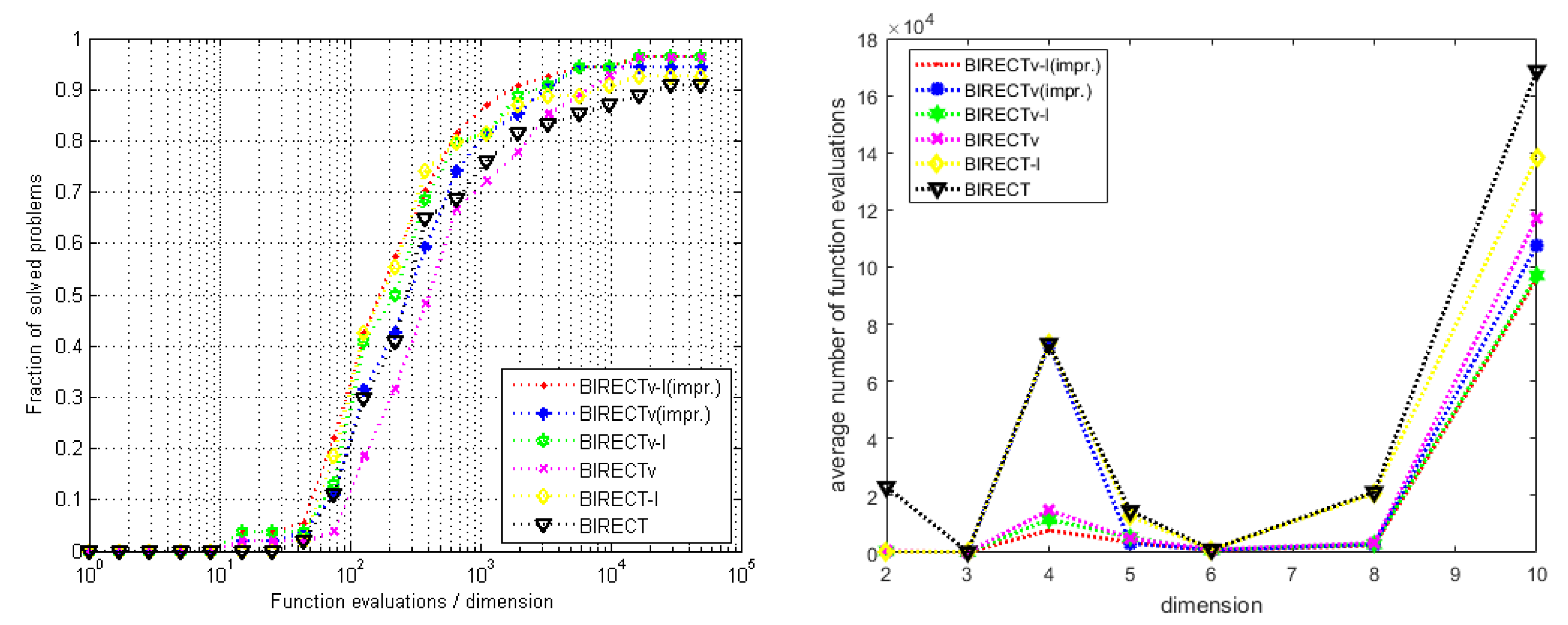
4.3. Examining the Success Rate of Algorithms and Function Evaluation Metrics

The graphical representations on the left side of Figure 4 furnish a comprehensive overview of the algorithmic performance under the prescribed computational limitations. Within a limited budget of function evaluations not exceeding $5\times {10}^5$, the number of evaluations for each test problem was set as $=n\times {10}^k$, where n is the problem dimension, and $0\le k\le 4+{log}_{10}5$. The parameter $k=h\times i$ varied with a step-size $h=(4+{log}_{10}5)/20$, and $i=0,1,\dots ,20$. The maximum number of function evaluations was reached for $n=10$, and $k=4+{log}_{10}5$, which exactly gives $5\times {10}^5=n\times {10}^k$. We computed the percentage of the test problems for each algorithm to achieve successful solution. We can observe that all algorithms failed when $0\le k\le 4\times h$. However, the success rates of all algorithms exhibited a gradual ascent within evaluations, from the value $k=5\times h$, even with quite small rates, except the algorithm BIRECT that remained at a low level until the value $k=7\times h$. For the value of $k=11\times h$, the success rate for three DIRECT-type algorithms (BIRECTv(impr.), BIRECT-l, and BIRECTv-l) exceeded the threshold of $50\%$ in solving the test problems, while the remaining algorithms were below this threshold. When the budget of function evaluations was expanded to the prescribed limit of $5\times {10}^5$ maximum, the BIRECTv-l(impr.) algorithm achieved the highest success rate with $90\%$, closely followed by BIRECTv(impr.), for $k=14\times h$, and the two BIRECTv-l, and BIRECT-l algorithms, BIRECT-l for $k=15\times h$, consistently maintaining the highest success rate among all the six algorithms. The remaining algorithms were BIRECTv with $k=17\times h$, and last BIRECT with $k=19\times h$. We observe that, for $i=20$, we can count a total of 21 points in the graphical representation for all methods.

To investigate the impact of dimensionality on the number of evaluations of the objective function, we have categorized all the problems in Table 1 based on their dimensions. Subsequently, we computed the average number of evaluations for each algorithm and represent the results graphically on the right side of Figure 4. It is evident from the analysis that the BIRECT algorithm yielded the least favorable results across all dimensions, followed by the BIRECT-l and BIRECTv algorithms. Conversely, the most favorable outcomes were observed with the two algorithms BIRECT-l(impr.) and BIRECTv-l, followed by the BIRECTv(imp) algorithm. Figure 4 also indicates that all algorithms faced challenges in the case of dimension 4. This issue is attributed to the presence of challenging test problems with this dimension.

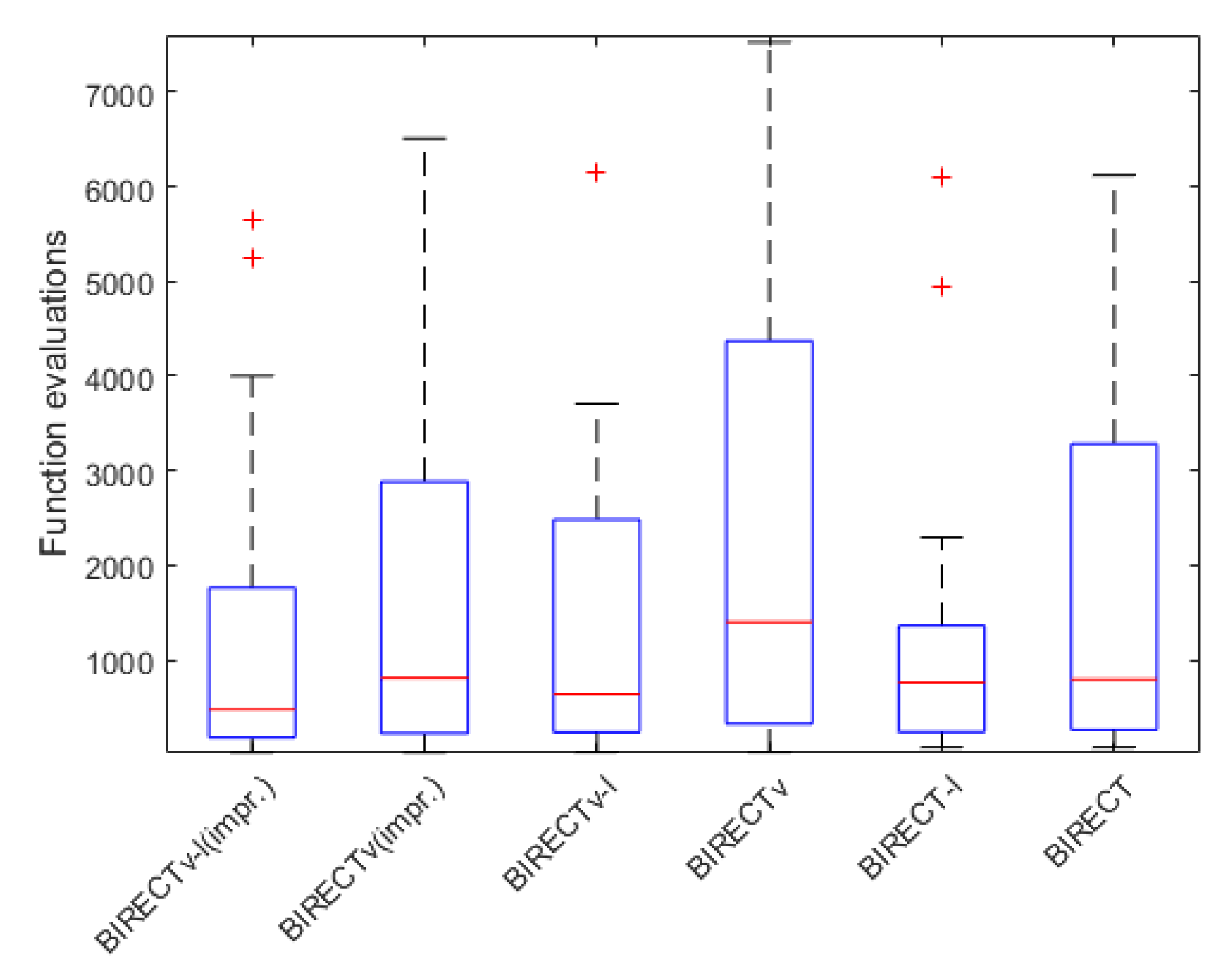
4.4. Statistical Analysis of the Results

The results of the algorithms on the benchmarks are presented in

Table 4. The statistical characteristics using different objective function evaluation budgets.

Algorithm	BIRECTv-l(impr.)	BIRECTv(impr.)	BIRECTv-l	BIRECTv	BIRECT-l	BIRECT
Success	$\mathbf{96.296}$	$94.444$	$\mathbf{96.296}$	$\mathbf{96.296}$	$92.593$	$90.741$
Fails	$\mathbf{3.704}$	$5.556$	$\mathbf{3.704}$	$\mathbf{3.704}$	$7.407$	$9.259$
max f.eval.	$\mathbf{28,871}$	$\mathrm{55,701}$	$\mathrm{38,460}$	$\mathrm{84,784}$	$\mathrm{66,462}$	$\mathrm{265,002}$
min f.eval.	$\mathbf{25}$	$\mathbf{25}$	28	28	80	80
average f.eval.	$\mathbf{2263.143}$	$4734.898$	$3006.980$	$8208.653$	$3886.755$	$\mathrm{11,106.714}$
Standard Deviation (std)	$\mathbf{5196.638}$	$\mathrm{11,027.286}$	$6965.689$	$\mathrm{17,874.922}$	$\mathrm{11,833.665}$	$\mathrm{39,800.355}$
median f.eval.	$\mathbf{480.000}$	$809.000$	$638.000$	$1400.000$	$764.000$	$794.000$

, where bold font indicates the best performance. In terms of algorithmic performance assessed through statistical characteristics, the proposed BIRECTv-l(impr.) consistently outperformed all other algorithms across all test problems. BIRECTv-l and BIRECT excelled in success and failure rates, securing the top positions. BIRECTv-l(impr.) attained the highest results in only one specific characteristic (min .eval.). Additionally, certain values of BIRECT-l and BIRECT are deemed insignificant. When considering standard deviation and median, BIRECTv-l(impr.) stands out as the optimal performer, closely followed by BIRECTv-l. In conclusion, both aspects underscore the superior performance of the proposed BIRECTv-l(impr.).

To evaluate the stability of the various algorithms from Table 4, we present a boxplot depicting the results in Figure 5. The central line of the BIRECT-vl(impr.) algorithm boxplot consistently exhibits the lowest values across all datasets, indicating exceptionally accurate results. Additionally, the proposed BIRECT-vl(impr.) algorithm exhibits fewer outliers.

Considering the outcomes of the Friedman mean rank test presented in

Table 5. Friedman mean rank values, using different objective function evaluation budgets.

Algorithm	$\mathit{n}\times {10}^{{\mathit{k}}_6}$	$\mathit{n}\times {10}^{{\mathit{k}}_7}$	$\mathit{n}\times {10}^{{\mathit{k}}_8}$	$\mathit{n}\times {10}^{{\mathit{k}}_9}$	$\mathit{n}\times {10}^{{\mathit{k}}_{10}}$
BIRECTv-l(impr.)	2.313	2.321	2.398	2.344	2.327
BIRECTv(impr.)	3.594	3.641	3.636	3.531	3.541
BIRECTv-l	4.031	3.987	4.011	3.938	3.888
BIRECTv	5.250	5.282	5.273	5.229	5.224
BIRECT-l	2.594	2.513	2.432	2.563	2.571
BIRECT	3.219	3.256	3.250	3.396	3.449
p-value	$4.0031\times {10}^{-10}$	$6.3283\times {10}^{-13}$	$1.2718\times {10}^{-14}$	$8.7793\times {10}^{-15}$	$5.4166\times {10}^{-15}$

, BIRECT-vl(impr.) secured the top rank across all budget levels in the objective function evaluation. The evaluation budgets are expressed as $n\times {10}^{k_i}$, where n represents the problem dimension, $k_i$ is calculated as $i\times (4+{log}_{10}5)/10$, and $i=6,7,8,9,10$. As an example, for $k_{10}$ and $n=10$, we obtained $n\times {10}^{k_i}=10\times {10}^{k_{10}}=\mathrm{500,000}$. Notably, the algorithm proved most beneficial with smaller evaluation budgets. The conducted Friedman test, at a 5% significance level, revealed significant performance differences among the various algorithms. As the evaluation budgets were increased, the Friedman mean rank values displayed diminished variability, indicating a convergence point where the algorithms may demonstrate comparable performance.

The significance levels (p-values) obtained from the Wilcoxon signed test, with a 5% threshold, were analyzed for BIRECTv-l(impr.) compared to the other competitors across various objective function evaluation budgets (see

Table 6. p-values (5% significance) of Wilcoxon signed test: BIRECTv-l(impr.) vs. competitors at various evaluation budgets $n\times {10}^{k_i}$.

Algorithm	$\mathit{n}\times {10}^{{\mathit{k}}_6}$	$\mathit{n}\times {10}^{{\mathit{k}}_7}$	$\mathit{n}\times {10}^{{\mathit{k}}_8}$	$\mathit{n}\times {10}^{{\mathit{k}}_9}$	$\mathit{n}\times {10}^{{\mathit{k}}_{10}}$
BIRECTv(impr.)	$3.210169\times {10}^{-4}$	$7.024763\times {10}^{-4}$	$1.683462\times {10}^{-3}$	$1.683462\times {10}^{-3}$	$1.683462\times {10}^{-3}$
BIRECTv-l	$5.249434\times {10}^{-8}$	$7.609271\times {10}^{-9}$	$3.520127\times {10}^{-9}$	$3.520127\times {10}^{-9}$	$3.520127\times {10}^{-9}$
BIRECTv	$7.190828\times {10}^{-6}$	$4.480184\times {10}^{-7}$	$2.046605\times {10}^{-7}$	$5.146379\times {10}^{-8}$	$5.146379\times {10}^{-8}$
BIRECT-l	$2.975178\times {10}^{-1}$	$3.657377\times {10}^{-1}$	$2.875319\times {10}^{-1}$	$6.049617\times {10}^{-1}$	$6.049617\times {10}^{-1}$
BIRECT	$4.005684\times {10}^{-1}$	$2.348613\times {10}^{-1}$	$2.892280\times {10}^{-1}$	$1.383033\times {10}^{-1}$	$9.273076\times {10}^{-2}$

). If the p-value exceeds $0.05$, this implies insignificance in the difference between the results of the two methods. However, in few cases, the p-values were below $0.05$, indicating a weak significance in the performance of the BIRECTv-l(impr.) algorithm compared to the alternative techniques.

5. Conclusions and Future Prospects

This paper introduced a novel DIRECT-type algorithm, BIRECTv. Incorporating recent partitioning and selection techniques proved essential for enhancing its performance in addressing global optimization problems. The improvements demonstrated that BIRECTv outperformed existing DIRECT-type algorithms, displaying higher efficiency and superior performance in terms of convergence rates and the number of required function evaluations.

In contrast, the conventional DIRECT-type algorithms often exhibited slower convergence rates and required a significantly higher number of function evaluations, particularly when the optimal solution lay at the boundaries of feasibility. The effectiveness of BIRECTv relies on sampling points at the vertices of hyper-rectangles. While heavily depending on vertex sampling may limit its performance in scenarios where the optimal solution is not near the hyper-rectangle vertices, this limitation was addressed in [29] by applying a mapping technique to the BIRECTv algorithm to eliminate infeasibility. Consequently, computations are confined to valid solutions within the feasible region defined by linear constraints.

The experimentation results confirmed the algorithm’s superior performance, especially in cases where solutions were located at the boundary of feasible regions. This research opens up new possibilities for addressing global optimization problems, suggesting that BIRECTv has the potential to make significant contributions in this field. The new algorithm is expected to occupy a pivotal place among all DIRECT-type algorithms, possibly becoming a standard choice for solving global optimization problems with the mentioned characteristics.

In conclusion, this paper lays the groundwork for future research by proposing that BIRECTv opens up new possibilities, potentially leading to further advancements in the field. Future investigations will focus on expanding the comparison of the new algorithm with various algorithms, using different benchmarks. All these observations may be considered as potential directions for future research.

References

1. Ma, K.; Rios, L.M.; Bhosekar, A.; Sahinidis, N.V.; Rajagopalan, S. Branch-and-Model: A derivative-free global optimization algorithm. Comput. Optim. Appl. 2023, 85, 337–367. [Google Scholar]
2. Liuzzi, G.; Lucidi, S.; Piccialli, V. Exploiting derivative-free local searches in DIRECT-type algorithms for global optimization. Comput. Optim. Appl. 2016, 65, 449–475. [Google Scholar]
3. Stripinis, L.; Paulavičius, R. Gendirect: A generalized direct-type algorithmic framework for derivative-free global optimization. arXiv 2023, arXiv:2309.00835. [Google Scholar]
4. Stripinis, L.; Paulavičius, R. Lipschitz-inspired HALRECT algorithm for derivative-free global optimization. J. Glob. Opt. 2023, 88, 139–169. [Google Scholar]
5. Stripinis, L.; Paulavičius, R. An extensive numerical benchmark study of deterministic vs. stochastic derivative-free global optimization algorithms. arXiv 2022, arXiv:2209.05759. [Google Scholar]
6. Stripinis, L.; Paulavičius, R. Derivative-Free DIRECT-Type Global Optimization: Applications and Software; Springer Nature: Cham, Switzerland, 2023. [Google Scholar]
7. Floudas, C.A. Deterministic Global Optimization: Theory, Methods and Applications; Springer Science & Business Media: Berlin/Heidelberg, Germany, 2013; Volume 37. [Google Scholar]
8. Horst, R.; Pardalos, P.M.; Thoai, N.V. Introduction to Global Optimization; Nonconvex Optimization and Its Application; Kluwer Academic Publishers: Berlin, Germany, 1995. [Google Scholar]
9. Horst, R.; Tuy, H. Global Optimization: Deterministic Approaches; Springer: Berlin/Heidelberg, Germany, 1996. [Google Scholar]
10. Sergeyev, Y.D.; Kvasov, D.E. On deterministic diagonal methods for solving global optimization problems with Lipschitz gradients. In Optimization, Control, and Applications in the Information Age: In Honor of Panos M. Pardalos’s 60th Birthday; Springer International Publishing: Berlin/Heidelberg, Germany, 2015; pp. 315–334. [Google Scholar]
11. Sergeyev, Y.D.; Kvasov, D.E. Deterministic Global Optimization: An Introduction to the Diagonal Approach; SpringerBriefs in Optimization; Springer: Berlin, Germany, 2017. [Google Scholar] [CrossRef]
12. Liberti, L.; Kucherenko, S. Comparison of deterministic and stochastic approaches to global optimization. Int. Oper. Res. 2005, 12, 263–285. [Google Scholar]
13. Zhigljavsky, A.; Žilinskas, A. Stochastic Global Optimization; Springer: New York, NY, USA, 2008. [Google Scholar]
14. Paulavičius, R.; Sergeyev, Y.D.; Kvasov, D.E.; Zilinskas, J. Globally-biased DISIMPL algorithm for expensive global optimization. J. Glob. Optim. 2014, 59, 545–567. [Google Scholar]
15. Paulavičius, R.; Zilinskas, J. Simplicial Lipschitz optimization without Lipschitz constant. J. Glob. Optim. 2014, 59, 23–40. [Google Scholar]
16. Paulavičius, R.; Žilinskas, J.; Grothey, A. Parallel branch and bound for global optimization with combination of Lipschitz bounds. Optim. Methods Softw. 2011, 26, 487–498. [Google Scholar]
17. Paulavičius, R.; Žilinskas, J. Simplicial Global Optimization; Springer: New York, NY, USA, 2014. [Google Scholar]
18. Sergeyev, Y.D. Efficient strategy for adaptive partition of N-dimensional intervals in the framework of diagonal algorithms. J. Optim. Theory Appl. 2000, 107, 145–168. [Google Scholar]
19. Sergeyev, Y.D. Efficient partition of N-dimensional intervals in the framework of one-point-based algorithms. J. Optim. Appl. 2005, 124, 503–510. [Google Scholar]
20. Sergeyev, Y.D.; Kvasov, D.E. Global search based on efficient diagonal partitions and a set of Lipschitz constants. SIAM J. Optim. 2006, 16, 910–937. [Google Scholar]
21. Jones, D.R.; Perttunen, C.D.; Stuckman, B.E. Lipschitzian optimization without the Lipschitz constant. J. Optim. Appl. 1993, 79, 157–181. [Google Scholar]
22. Jones, D.R. The DIRECT global optimization algorithm. In The Encyclopedia of Optimization; Floudas, C.A., Pardalos, P.M., Eds.; Kluwer Academic Publishers: Dordrect, The Netherlands, 2001; pp. 431–440. [Google Scholar]
23. Stripinis, L.; Paulavičius, R.; Žilinskas, J. Improved scheme for selection of potentially optimal hyper-rectangles in DIRECT. Optim. Lett. 2018, 12, 1699–1712. [Google Scholar]
24. Stripinis, L.; Paulavičius, R. An empirical study of various candidate selection and partitioning techniques in the DIRECT framework. J. Glob. Optim. 2022, 1–31. [Google Scholar]
25. Jones, D.R.; Martins, J.R.R.A. The DIRECT algorithm: 25 years Later. J. Glob. Optim. 2021, 79, 521–566. [Google Scholar]
26. Paulavičius, R.; Sergeyev, Y.D. Globally-biased BIRECT algorithm with local accelerators for expensive global optimization. Expert Syst. Appl. 2020, 144, 113052. [Google Scholar]
27. Guessoum, N.; Chiter, L. Diagonal Partitioning Strategy Using Bisection of Rectangles and a Novel Sampling Scheme. MENDEL 2023, 29, 131–146. [Google Scholar]
28. Liu, H.; Xu, S.; Wang, X.; Wu, J.; Song, Y. A global optimization algorithm for simulation-based problems via the extended DIRECT scheme. Eng. Optim. 2015, 47, 1441–1458. [Google Scholar]
29. Stripinis, L.; Paulavičius, R. Novel algorithm for linearly constrained derivative free global optimization of lipschitz functions. Mathematics 2023, 11, 2920. [Google Scholar]
30. Chiter, L. Experimental Data for the Preprint “Diagonal Partitioning Strategy Using Bisection of Rectangles and a Novel Sampling Scheme”. Mendeley Data, V2. 2023. Available online: https://data.mendeley.com/datasets/x9fpc9w7wh/2 (accessed on 16 June 2023).
31. Friedman, M. The Use of Ranks to Avoid the Assumption of Normality Implicit in the Analysis of Variance. J. Am. Stat. Assoc. 1937, 32, 675–701. [Google Scholar]
32. Hollander, M.; Wolfe, D. Nonparametric Statistical Methods, Solutions Manual; Wiley Series in Probability and Statistics; Wiley: Hoboken, NJ, USA, 1999. [Google Scholar]
33. Phan, D.T.; Liu, H.; Nguyen, L.M. StepDIRECT-A Derivative-Free Optimization Method for Stepwise Functions. In Proceedings of the 2022 SIAM International Conference on Data Mining (SDM), Society for Industrial and Applied Mathematics, Alexandria, VA, USA, 28–30 April 2022; pp. 477–485. [Google Scholar]
34. Stripinis, L.; Paulavičius, R. Experimental Study of Excessive Local Refinement Reduction Techniques for Global Optimization DIRECT-Type Algorithms. Mathematics 2022, 10, 3760. [Google Scholar] [CrossRef]
35. Gablonsky, J.M.; Kelley, C.T. A locally-biased form of the DIRECT algorithm. J. Glob. Optim. 2001, 21, 27–37. [Google Scholar]
36. Baker, C.A.; Watson, L.T.; Grossman, B.M.; Mason, W.H.; Haftka, R.T. Parallel Global Aircraft Configuration Design Space Exploration; High Performance Computing Symposium 2000; Tentner, A., Ed.; Soc. for Computer Simulation Internat: Blacksburg, VA, USA, 2000; pp. 54–66. [Google Scholar]
37. Mockus, J.; Paulavičius, R.; Rusakevixcxius, D.; Sešok, D.; Žilinskas, J. Application of Reduced-set Pareto-Lipschitzian Optimization to truss optimization. J. Glob. Optim. 2017, 67, 425–450. [Google Scholar]
38. Liu, Q.; Zeng, J.; Yang, G. MrDIRECT: A multilevel robust DIRECT algorithm for global optimization problems. J. Glob. Opt. 2015, 62, 205–227. [Google Scholar]
39. Stripinis, L.; Kůdela, J.; Paulavičius, R. DIRECTGOLib—Direct Global Optimization Test Problems Library. 2023. Available online: https://github.com/blockchain-group/DIRECTGOLib (accessed on 16 June 2023).
40. Stripinis, L.; Paulavičius, R. DIRECTGO: A new DIRECT-type MATLAB toolbox for derivative-free global optimization. ACM Trans. Math. Softw. 2022, 48, 1–46. [Google Scholar]
41. Paulavičius, R.; Chiter, L.; Žilinskas, J. Global optimization based on bisection of rectangles, function values at diagonals, and a set of Lipschitz constants. J. Glob. Optim. 2018, 71, 5–20. [Google Scholar]
42. Tuy, H. Convex Analysis and Global Optimization; Springer Science & Business Media: Berlin/Heidelberg, Germany, 2013. [Google Scholar]
43. Tsvetkov, E.A.; Krymov, R.A. Pure Random Search with Virtual Extension of Feasible Region. J. Optim. Theory Appl. 2022, 195, 575–595. [Google Scholar]
44. Hedar, A. Test Functions for Unconstrained Global Optimization; System Optimization Laboratory, Kyoto University: Kyoto, Japan, 2013; Available online: http://www-optima.amp.i.kyotou.ac.jp/member/student/hedar/Hedar_files/TestGO.htm (accessed on 26 February 2021).
Figure 1. Description of the initialization and the first two iterations used in two different sampling and partitioning schemes (BIRECT: upper figure), and (BIRECTv: lower figure) on a two-dimensional example.
Mathematics 12 00283 g001
Figure 2. Grouping strategy using two different tolerance levels in the BIRECT algorithm applied to the Ackley test problem 1 at iteration 36. Small tolerance (left side), large tolerance (right side).
Mathematics 12 00283 g002
Figure 3. An example of the iteration progress using the BIRECTv algorithm on the left-hand side from [27], and Impr.BIRECTv(impr.) on the right-hand side, while solving the Branin test problem (No. 3 from Table 1).
Mathematics 12 00283 g003
Figure 4. Profiles of data and performance metrics for evaluating function performance across various problems from Table 1.
Mathematics 12 00283 g004
Figure 5. Boxplots of the results for all algorithms.
Mathematics 12 00283 g005