Adaptive Graph Attention and Long Short-Term Memory-Based Networks for Traffic Prediction

Abstract

While the increased availability of traffic data is allowing us to better understand urban mobility, research on data-driven and predictive modeling is also providing new methods for improving traffic management and reducing congestion. In this paper, we present a hybrid predictive modeling architecture, namely GAT-LSTM, by incorporating graph attention (GAT) and long short-term memory (LSTM) networks for handling traffic prediction tasks. In this architecture, GAT networks capture the spatial dependencies of the traffic network, LSTM networks capture the temporal correlations, and the Dayfeature component incorporates time and external information (such as day of the week, extreme weather conditions, holidays, etc.). A key attention block is designed to integrate GAT, LSTM, and the Dayfeature components as well as learn and assign weights to these different components within the architecture. This method of integration is proven effective at improving prediction accuracy, as shown by the experimental results obtained with the PeMS08 open dataset, and the proposed model demonstrates state-of-the-art performance in these experiments. Furthermore, the hybrid model demonstrates adaptability to dynamic traffic conditions, different prediction horizons, and various traffic networks.

1. Introduction

Closely tied to the development of transportation systems and the growing need to address traffic congestion-related problems in urban areas, traffic prediction now plays a vital role in traffic management, congestion reduction, transportation planning, and improvements in public services. Thus, traffic prediction is a crucial component of intelligent transportation systems (ITS) and broader smart city frameworks. On the other hand, the use of more data generated with the ITS infrastructure and advanced technologies applied to transportation systems promotes the use of new traffic prediction methods, e.g., in recent years, traffic prediction capabilities have been significantly enhanced through the integration of machine learning techniques and big data analytics.

Before 2010, traffic prediction methods primarily relied on traditional modeling approaches and statistical techniques, such as time series analysis, regression analysis, autoregressive integrated moving average (ARIMA), and modeling and forecasting traffic in a simulated environment like the traffic simulation software VISSIM. ARIMA and its variants [1,2,3] are some of the consolidated early learning models most widely used as baseline models for developing new approaches. Through the application of the support vector machine (SVM) method to time series, supervised machine learning models with support vector regression (SVR) can also be applied to traffic data analysis, e.g., an SVR predictor was proposed for use in travel-time prediction in [4], while an online SVR was used to predict traffic flow in both typical and non-recurring atypical traffic conditions in [5]. K-nearest neighbor (KNN) models [6,7] are another type of nonparametric regression method applied for short-term traffic forecasting. Moreover, we have observed a shift towards more data-driven and sophisticated approaches in the post-2010 period, leveraging advanced computational techniques to improve the accuracy and timeliness of traffic predictions. In particular, the application of deep learning models has played an important role in advancing the field of traffic data analysis and the prediction of traffic conditions. Researchers in [8] proposed a stacked autoencoder (SAE) model integrated with a greedy layer-wise unsupervised learning algorithm to pre-train deep networks, reporting that the proposed SAE method can discover the latent traffic flow feature representation, such as the nonlinear spatial and temporal correlations from the traffic data. The long short-term memory (LSTM) neural network is a type of recurrent neural network (RNNs) capable of capturing long-term dependencies in sequential data. Reference [9] is one of the previous studies that applied LSTM neural networks to traffic prediction tasks, demonstrating that the LSTM model is effective for short-term travel speed prediction without requiring prior information about the time lag. In addition, it has a superior capability for time series prediction with long temporal dependency. Due to its competitive performance, the LSTM method is often regarded as a baseline in subsequently proposed approaches. Meanwhile, ever-more enhanced LSTM models [10,11] and hybrid LSTM-based models [12,13,14,15,16,17] have been proposed.

Convolutional neural networks (CNNs) have also been applied for modeling spatial-temporal traffic data to capture the temporal dependencies or spatial correlations in traffic networks [18,19,20,21]. However, traditional CNNs are often limited to modeling Euclidean data, and graph convolutional networks (GCNs) have gained popularity since 2018, as traffic data usually have non-Euclidean spatial structures and can be represented in graph form. The diffusion convolutional recurrent neural network (DCRNN) [22] is an existing model that uses graph convolutions to capture the spatial dependency and recurrent neural networks (with an encoder-decoder architecture) for temporal dependency, and it has been demonstrated that this combination can achieve better performance than statistical models and pure RNNs-based models. Similarly, another GCN-RNN hybrid model named the temporal graph convolutional network (T-GCN) [23] was proposed for learning the complex topological structures of traffic networks and dynamic changes in traffic data, where the RNN layer was a gated recurrent unit (GRU). An early spatial-temporal graph convolutional network (STGCN) [24] was also designed by combining graph convolutions and gated temporal convolutions to extract spatial features and temporal features in parallel. In [25], two parallel GCN branches were used in the dual-channel GCN model (DC-STGCN), where the GCN branches captured both spatial and temporal dependencies in traffic data. Other than using separated modules to capture spatial and temporal features, Song et al. proposed a spatial-temporal synchronous graph convolutional network (STSGCN) [26] to capture localized spatial-temporal correlations at the same time. Other frequently cited models based on graph structure data include the graph wavenet recurrent neural network (Graph WaveNet) [27], the attention-based spatial–temporal graph convolutional network (ASTGCN) [28], and the graph multi-attention network (GMAN) [29].

Notably, when the ASTGCN model was proposed in [28], its performance was superior to those of models that existed at that time. At almost the same time, the Graph WaveNet achieved state-of-the-art results [27], outperforming ARIMA, FC-LSTM, DCRNN, and STGCN. Moreover, interestingly, in the next year, when STSGCN and GMAN were each proposed, the STSGCN model [26] was found to have a better performance than ASTGCN for four datasets collected from the Caltrans Performance Measurement System (PeMS), and the GMAN model [29] achieved even better results than the Graph WaveNet model and other previous models (especially when the prediction horizon tended to be longer) from two datasets (one from Xiamen and the other from PeMS). To date, the trend of using architectures that integrate graph convolution or graph attention with temporal prediction models, such as LSTM networks and GRU networks, for handling traffic prediction tasks has continued.

Recently, hybrid models that integrate the application of adaptive graph representation [30,31,32] and multi-graph models [33,34] have been used to achieve higher accuracy in prediction techniques. Graph WaveNet [27] uses a self-adaptive adjacency matrix to capture hidden spatial dependencies as well as dilated casual convolution networks to capture long temporal trends. In [15], DyGCN uses a dynamic distance correlation temporal graph-based adjacency matrix as an alternative to the static spatial distance matrix to capture the spatial correlations of neighboring and relevant remote sensors. Another hybrid model, namely TYRE [31], uses GCN with gating and attention mechanisms as an intra-graph model and generates node embeddings at each time point to learn the temporal dependency. Three graph structures (connectivity, similarity, and betweenness) were firstly fused by attention in the ETGCN [33] model before integrating the graph convolutional network and gated recurrent unit to identify spatial and temporal dependencies. These approaches enable more accurate forecasting through the analysis of large datasets, considering various influencing factors and adapting to changing conditions.

However, we still face the following challenges related to applying these deep learning approaches to traffic prediction tasks:

• Generally, the prediction accuracy decreases as the prediction horizon increases, with this trend noted in almost all prediction models.
• Super parameters configured for a specific model may have significant impacts on its prediction performance. Researchers often need to spend a great deal of time and effort to tune model parameters and obtain the optimal modeling results based on certain expert experience.
• Furthermore, when varying the spatial and temporal dependencies between one traffic network and another, a well-tuned model with specific parameters may have different performance for a new dataset application scenario.

Therefore, dynamically calculating the similarity matrix and updating attention weights are the two main adaptive techniques used for handling traffic prediction problems. In this study, we propose a general GAT-LSTM architecture by combining state-of-the-art graph attention networks and long short-term memory networks to capture spatial and temporal dependencies from traffic data, which are collected by sensors installed in road networks. Moreover, we intend to introduce other relevant data into our model to improve its prediction accuracy. For example, the traffic state may change significantly due to uncertainties, such as accidents and important local events, and we may model some of these uncertainties to improve the prediction performance of the model. To enhance our model, we also propose using an attention block to learn the contributions of GAT networks and other original inputs to the whole model on the basis of specific sensor (node) locations.

The main contributions of this work are summarized as follows:

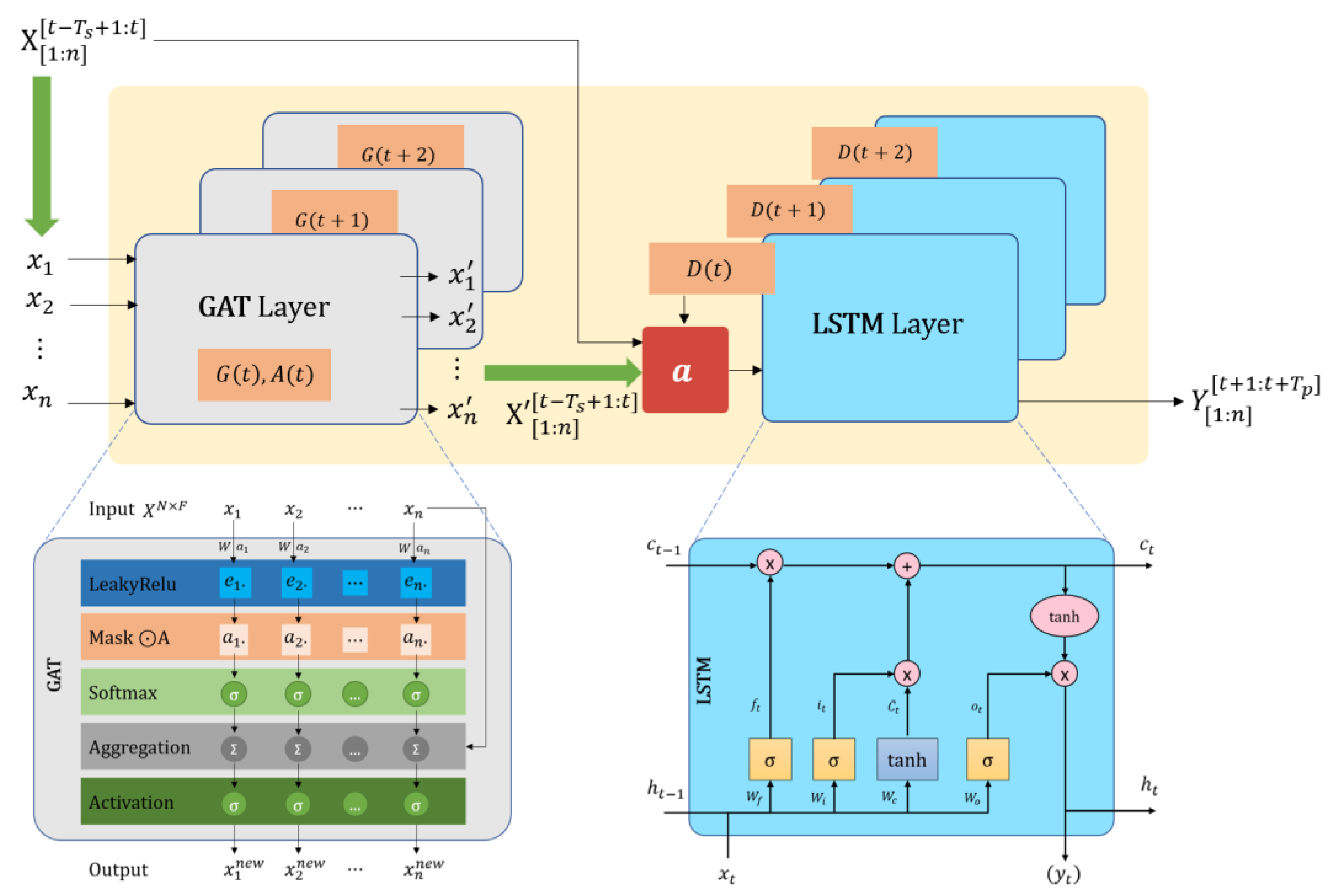
• We propose a novel GAT-LSTM architecture that is applicable to both global and local graphs, according to the road network and prediction tasks. In this architecture, an extra input called Dayfeature is designed to include external factors affecting traffic conditions, such as extreme weather, public holidays, and other special uncertainties that may arise over time, which greatly improves the prediction accuracy.
• The GAT network and LSTM network are not simply connected in series within the model. An attention block is designed to learn the weights of the GAT network, original traffic data, and Dayfeature before passing them into the LSTM network. These weights vary from one node to another. Thus, within the global GAT-LSTM model, the GAT network and LSTM network may automatically have different combinations to adaptively predict traffic conditions for each local sensor. This design also allows the model to be easily applied to other traffic networks using new datasets.
• The proposed model achieved state-of-the-art performance in traffic flow prediction using the PeMS08 open dataset (also known as PeMSD8 in some literature). In addition, weaker nodes within the traffic network can be detected, and local adaption algorithms can be designed to further improve the local performance of the model.

The remainder of the paper is organized as follows. The model definition and the main architecture of GAT-LSTM networks are introduced in Section 2. Then, we outline the experiments, analyze the experimental results, and describe the adaptive mechanism in Section 3. A brief discussion of the factors influencing the results is carried out in Section 4, and the conclusions of our work and ongoing research lines are presented in Section 5.

2. Methods

2.1. Problem Description

Traffic prediction involves forecasting the future states of traffic flow, speed, congestion, and other related variables in a given area using historical traffic data while also considering other features that impact traffic conditions, such as weather conditions, special events, road infrastructure, etc.

2.1.1. Traffic Network Graphs

We define the general spatial traffic network as a graph $G=\left(V, A\right)$, where $\mathrm{V}$ is the whole set of nodes that corresponds to the $\mathrm{N}$ sensors in the traffic network, and $\mathrm{A}\left(\mathrm{A}\in {ℝ}^{N\times N}\right)$ is the adjacency matrix corresponding to the connectivity and other dynamic correlations between nodes. The graph of a given area of a traffic network is generally stable, with variability only occurring during situations such as infrastructure construction (or reconstruction) and the temporary closure of roads. However, these temporary changes can result in variations in traffic patterns, thus affecting the prediction accuracy. To take these special cases into account, we consider the graph to be dynamic and use $G\left(t\right)=\left(V, A\left(t\right)\right)$ to denote the traffic network at current time $t$. A subgraph $G_i\left(t\right)=\left(V_i, A_i\left(t\right)\right)$ is defined as representing a distributed point in our previous work, which is linked to a central node $i \left(i\in V\right)$; here, $V_i$ is the subset of $N_i$ nodes ($N_i\le N$) that includes node $i$ and its neighbors, and $A_i\left(t\right)$ is the local adjacency matrix at time $t$.

Recently, different types of adjacency matrices have been proposed to construct multiple graphs for GNNs, such as matrices based on the spatial distance between nodes [33,34]; localized neighborhood connectivity [26,35,36]; similarity [15,33], which is the temporal graph-based correlations between the time series of pairs of nodes; and betweenness [33], which determines the degree of busyness of a road section passed through by all shortest routes between a pair of nodes. We use the dynamic connectivity adjacency matrix $A_C\left(t\right)$. It is defined based on the existence of edges or links between pairs of nodes, i.e., the road connections between pairs of sensors in specific direction. As properties of the road network, these adjacency relationships are generally consistently maintained, with alterations only occurring in specific restrictive conditions. The dynamic connectivity adjacency matrix is defined as follows:

$$A_{C,i,j}(t)=\{\begin{array}{l}1,if node j is an outgoing neighbor from ndde i at time t, i\ne j\\ 0,otherwise\end{array}$$

(1)

2.1.2. Traffic States

We use $X^t\left(X^t\in {ℝ}^{N\times F}\right)$ and $x_i^t\left(x_i^t\in X^t\right)$ to denote the traffic states of all the nodes and the traffic state of a single node $i$ at current time $t$, respectively. $F$ represents the number of features. In this paper, we only use one traffic feature to represent traffic state (i.e., $F=1$), and this traffic feature can be average speed, traffic volume, traffic intensity, etc.

2.1.3. Temporal and Other External Features

Temporal features include the hour of the day, the day of the week, holidays, public vacation time, etc., and possible external features taken into consideration are extreme weather, important local events, etc. These features are encoded into a feature matrix $D\left(t\right)$, which, in this paper, we called Dayfeature.

2.1.4. Problem

We set $X^{\left[t-T_s+1:t\right]}$ as the historical state sequences of all nodes for the last $T_s$ time slots and set $X^{\left[t+1:t+T_p\right]}$ as the future states for the next $T_p$ time slots; thus, the traffic prediction problem is represented by

$$\left(X^{\left[t-T_s+1:t\right]},G\left(t\right),D\left(t\right)\right)\stackrel{M}{\to } Y^{\left[t+1:t+T_p\right]}$$

(2)

where $M$ is the model used for traffic prediction, and $Y^{\left[t+1:t+T_p\right]}$ are the predicted state sequences.

2.2. GAT-LSTM Model

GAT-LSTM is an integrated neural network architecture designed for the joint modeling of traffic data that may possess both graph-structured features and sequential dependencies. This hybrid model combines the strengths of the graph attention network for capturing spatial relationships in graph data and long short-term memory for modeling temporal dependencies in sequential data. In this study, the distribution of sensors and the connectivity of the traffic network are represented by graphs, and the traffic states of the sensors are represented by parallel sequences. The proposed GAT-LSTM model is shown in Figure 1. Here, the GAT layers apply the attention mechanism to assign importance weights to the neighboring nodes, which are actually relevant for central nodes during the traffic state propagation, and the LSTM layers adaptively combine the GAT weights and original traffic sequences to learn the temporal long-term and short-term traffic patterns of each node.

A GAT layer can be expressed as follows:

$$x_i^{’}=\begin{array}{c}K\\ \parallel \\ k=1\end{array}\sigma \left({{\displaystyle \sum }}_{j\in V_i}{\alpha }_{ij}^k\left(W^k·x_j\right)+b^k\right), x_j\in {ℝ}^{1\times F}$$

(3)

where $x_i^{’}$ is the weight assigned for node $i$ through the GAT layer with configured $K\left(K\ge 1\right)$ attention heads, $x_j\left(j\in V_i\right)$ is the input feature vector of node $i$ and its neighbors, $\sigma (·)$ is the activation function, $\parallel$ is the concatenation operation, and $W^k$ and $b^k$ are learnable parameters. Inspired by the graph attention networks proposed in [37], the attention coefficients are computed and normalized using Equations (4) and (5), respectively, as follows:

$$e_{ij}^k=LeakyReLU\left({(a^k)}^{⊺}·(W^k·x_j)\right)$$

(4)

$${\alpha }_{ij}^k=Softmax\left(Mask\left(e_{ij}^k,A_i\right)\right)$$

(5)

In Equation (4), $a^k$ is a shared and learnable attention parameter that captures the correlations of node features during attention calculation. We use the leaky rectified linear unit activation function LeakyReLU to calculate the attention coefficient $e_{ij}^k$ and Mask it with the dynamic (if available) adjacency matrix. LeakyReLU is a function applied to reduce the impacts of the negative values of features in the input data by multiplying a gradient coefficient when the input values are negative. We set 0.1 as the value of this gradient coefficient, while 0.2 was used in [37]. Mask is a function applied to update values satisfied by the condition $A_{C,ij}\left(t\right)>0$. Finally, another activation function, namely Softmax, is used to normalize the attention coefficients.

As shown in Figure 1, the outputs of GAT layers become part of the input data of LSTM layers. In GAT layers, the attention weights are calculated in a node-wise manner, and the attention heads are concatenated along the feature dimension. In order to capture different levels of temporal dependencies in the historical traffic data, the traffic data are sequentially operated over time steps in LSTM layers. However, not all nodes are equally dependent on the spatial network in which they are located. In other words, when we use GAT layers as the full inputs of LSTM layers, we may have overfitted the spatial dependency of some nodes. Thus, for innovation purposes, an attention-based block is designed in this model to fuse the output data of GAT layers, original traffic data, and Dayfeature data; thus, the inputs of LSTM layers are not limited to the GAT outputs. The GAT-LSTM mechanism of our proposed weighted GAT-LSTM model for each time step can be expressed using Equations (6)–(12).

$${𝓲}_t=\sigma \left(W_{xi}{x}_t+W_{hi}{h}_{t-1}+b_i\right)$$

(6)

$$f_t=\sigma \left(W_{xf}{x}_t+W_{hf}{h}_{t-1}+b_f\right)$$

(7)

$$c_t=f_t⨀c_{t-1}+{𝓲}_t⨀tanh\left(W_{xc}{x}_t+W_{hc}{h}_{t-1}+b_c\right)$$

(8)

$$o_t=\sigma \left(W_{xo}{x}_t+W_{ho}{h}_{t-1}+b_o\right)$$

(9)

$$h_t=o_t⨀tanh\left(c_t\right)$$

(10)

where $x_t$ is calculated using Equation (11): a weighted concatenation operation of the output of the GAT layer $GAT(·)$, traffic data input $X^t$, and the other feature matrix $D\left(t\right)$ (also see block $a$ in Figure 1).

$$x_t=a_x{X}^t\parallel a_{g}GAT\left(X^t\right)\parallel a_{d}D\left(t\right)$$

(11)

where $\parallel$ denotes concatenation. The corresponding weight vectors $a_x$,$a_g$, and $a_d$ are learnable and assignable, and for each node $i$, they satisfy the following equation:

$$a_{x,i}+a_{g,i}+a_{d,i}=1$$

(12)

3. Experiments

In this section, we design relevant experiments and evaluate the performance of the proposed model based on the PeMS08 open traffic dataset [26,28] from the Caltrans Performance Measurement System (PeMS).

3.1. Dataset and Baselines

The PeMS08 dataset, also known as PeMSD8 in some studies, is a highway traffic dataset collected at San Bernardino from 1 July to 31 August 2016 and includes the historical data of 170 detectors (derived from the original 1979 detectors by excluding those that were too closely positioned). The traffic data of each detector include three traffic features, namely traffic flow, average speed, and average occupancy, sequenced based on a frequency of 5 min. This dataset is one of the open datasets that is often used in traffic flow prediction research and has also been used in [14,26,28] to validate the LST-GCN, ASTGCN, and STSGCN models. These models are referred as baselines in this study.

As we discovered in Section 1, the models ASTGCN [28] and STSGCN [26] have been found to have better performance in traffic flow prediction than most of the other methods available at that time based on PeMS08 and other datasets, such as HA, ARIMA, VAR, LSTM, DCRNN, STGCN, etc. The LST-GCN model [14], which embeds LSTM networks into the training process of GCN networks, was reported to have achieved improvements compared to LSTM and ASTGCN. Thus, for representation, we use these models, including the attention-based spatial-temporal graph convolutional network (ASTGCN), spatial–temporal synchronous graph convolutional network (STSGCN), and LSTM-embedded graph convolution network (LST-GCN), and a two-layer stacked LSTM model as the baselines in this study.

3.2. Evaluation Metrics

Four metrics are used to study the performance of the proposed model and the baselines.

• Mean absolute error (MAE):

$$MAE=\frac{1}{T_p\times N}{\displaystyle \sum }_{\tau =1}^{T_p}{\displaystyle \sum }_{i=1}^N\left|x_i^{t+\tau }-y_i^{t+\tau }\right|$$

(13)

where $x_i^{t+\tau }\in X^{\left[t+1:t+T_p\right]}$ is the observed traffic state, and $y_i^{t+\tau }\in Y^{\left[t+1:t+T_p\right]}$ is the predicted value.

• Rooted mean square error (RMSE):

$$RMSE=\sqrt{\frac{1}{T_p\times N}{\displaystyle \sum }_{\tau =1}^{T_p}{\displaystyle \sum }_{i=1}^N{\left(x_i^{t+\tau }-y_i^{t+\tau }\right)}^2}$$

(14)

• Mean absolute percentage error (MAPE):

$$MAPE=\frac{1}{T_p\times N}{\displaystyle \sum }_{\tau =1}^{T_p}{\displaystyle \sum }_{i=1}^N\frac{\left|x_i^{t+\tau }-y_i^{t+\tau }\right|}{x_i^{t+\tau }}\times 100\%$$

(15)

where $x_i^{t+\tau }\ne 0$, i.e., only when the observed traffic states are not zero, the corresponding prediction results are calculated using the MAPE metric.

• However, the traffic state (flow, speed, or occupancy) can be equal to zero. To include these zero values, we introduce another metric to include all traffic states, namely the symmetric mean absolute percentage error (SMAPE):

$$SMAPE=\frac{1}{T_p\times N}{\displaystyle \sum }_{\tau =1}^{T_p}{\displaystyle \sum }_{i=1}^N\frac{\left|x_i^{t+\tau }-y_i^{t+\tau }\right|}{(x_i^{t+\tau }+y_i^{t+\tau })/2}\times 100\%$$

(16)

We utilize the fact that the predicted values are always positive after machine operations. It still can produce large values when the observations are extremely small or zero values.

3.3. Experimental Design

The dataset is divided into training, validation, and test sets at proportions of 65%, 15%, and 20%, respectively. The models are set to use one-hour historical data (with 12 time slots, i.e., $T_s=12$) to predict the traffic states at 15 min, 30 min, and 60 min ($T_p=3, 6, \mathrm{and} 12$, respectively).

To study the impact of the Dayfeature component on the forecasting task, we use a pair of two-layer stacked LSTM models, namely LSTM and LSTM_D, for experimental comparison. The sole distinction between these two LSTM models is that the LSTM_D model incorporates the Dayfeature input, whereas the LSTM does not. Another set of comparative models are GAT-LSTM_D and GAT-LSTM_D_a, two instances of the proposed GAT-LSTM architecture. GAT-LSTM_D includes the Dayfeature but excludes the attention block, where the GAT outputs, original traffic state sequences, and Dayfeature are parallel inputs of LSTM layers. In contrast, the GAT-LSTM_D_a has the attention block that dynamically assigns weights to these three types of inputs. Simultaneously, we integrate the four metrics to evaluate the general performance of the models involved in the experiments.

In addition to assessing the overall performance of the models by considering the average prediction accuracy across all nodes, we also investigate the performance of each model at the node level by analyzing the error metrics at different nodes. Furthermore, attentions assigned to different components within the proposed GAT-LSTM architecture are tracked for further analysis.

3.4. Results

3.4.1. Overall Performance on the Traffic Network

The MAE, RMSE, MAPE, and SMAPE metrics for the prediction results for 15, 30, and 60 min from the proposed model and the baseline models are shown in

Table 1. Metrics on prediction results for the 15 min, 30 min, and 60 min horizons.

	Metrics	MAE			RMSE			MAPE (%)			SMAPE (%)
Models		15 min	30 min	60 min	15 min	30 min	60 min	15 min	30 min	60 min	15 min	30 min	60 min
ASTGCN *				18.61			28.16			13.08			--
STSGCN *				17.13			26.80			10.96			--
LST-GCN **				17.93			27.47			12.81			--
LSTM		15.96	17.87	21.08	22.34	24.90	29.08	10.39	11.55	13.60	10.03	11.04	12.76
LSTM_D		17.95	18.38	18.99	24.96	25.60	26.34	11.73	11.90	12.26	11.21	11.36	11.67
GAT-LSTM_D		16.23	17.08	18.27	22.06	23.20	24.79	11.02	11.46	12.05	10.56	10.89	11.44
GAT-LSTM_D_a		15.32	16.24	17.16	21.05	22.69	24.21	10.39	11.02	11.51	10.39	10.56	10.93

* Results of ATSGCN and STSGCN are cited from [26]. ** Results of LST-GCN are cited from [14].

. The best results for these metrics according to the experiments are marked in bold.

From the comparative results, we find that the proposed GAT-LSTM model (GAT-LSTM_D_a) can achieve a better performance in 60 min traffic flow prediction for the PeMS08 dataset compared to LSTM, ATSGCN, and LST-GCN for the MAE, RMSE, and MAPE metrics as well as a competitive performance compared to STSGCN. We see that there is a marginal 5.02% difference from the best result achieved using STSGCN in the MAPE metric, but the results also showcase notable progress, with a substantial 9.66% improvement in the RMSE metric. These outcomes collectively support the assertion that the proposed model can be considered to be a state-of-the-art method in its domain.

Figure 2 presents a comparison of metrics for each prediction step across the following experimental models: LSTM, LSTM_D, GAT-LSTM_D, and GAT-LSTM_D_a. Generally, the prediction errors increase as the prediction horizon grows in all models. However, upon comparing the error lines of LSTM and LSTM_D, we see that the incorporation of Dayfeature substantially decreases the rate of error growth. For all metrics, within the context of fewer than three prediction steps, the inclusion of Dayfeature does not yield an advantage; instead, it contributes to an increase in the average errors. It is only when the number of prediction steps surpasses six that the average error associated with LSTM_D outperforms the average error of LSTM. This observation is particularly significant and promising for long-term prediction, as it indicates that the incorporation of Dayfeature has a positive impact in terms of mitigating error accumulation over extended forecasting periods. With Dayfeature included, GAT-LSTM_D and GAT-LSTM_D_a further reduce the error level to an even lower magnitude. Moreover, GAT-LSTM_D_a achieved an average prediction accuracy that surpassed those of the other three models within three prediction steps. This result indicates that the proposed model, i.e., GAT-LSTM_D_a, can be equally competitive in long-term and short-term forecasting. In traffic forecasting problems, short-term often means a forecast horizon of less than an hour, while long-term usually means a horizon of hours to days.

In addition, Figure 2 illustrates that MAE and RMSE exhibit comparable trends and contrasting effects, and MAPE and SMAPE display similar patterns. In the subsequent analysis, we will utilize only MAE and MAPE to present the remaining results. Meanwhile, we verified that SMAPE can serve as an alternative to MAPE, especially when the ground truth data include a significant number of zeros.

3.4.2. Node-Wise Performance

The assessment of the model’s overall performance relies on the average prediction errors of the entire traffic network. In this section, we conduct a detailed examination of the model’s node-wise performance. Figure 3 illustrates the experimental models’ MAE and MAPE distributions across the sensors (nodes) in the traffic network when $T_s=12$ and $T_p=12$ (the prediction horizon is 60 min). A model with superior overall performance across the network does not guarantee equal performance at all nodes. In Figure 3, GAT-LSTM_D_a achieved significant improvements at most nodes with the use of MAE, including nodes 4, 27, 70, 71,121, 143, 151, etc. However, it failed to make improvements or resulted in larger errors at some nodes compared to LSTM, such as nodes 28, 72, 127, 154, and 155 (labeled in red in Figure 3). Similar patterns are observed for RMSE, MAPE, and SMAPE. Moreover, by comparing the node-wise performance of GAT-LSTM_D and GAT-LSTM_D_a, we note that GAT-LSTM_D can reduce errors to levels below those of GAT-LSTM_D_a for nodes at which the errors are relatively small, such as nodes 70, 121 to 125, etc. However, GAT-LSTM_D_a plays a more significant role in minimizing errors at nodes where the errors are relatively large, such as nodes 4, 27, 71, 143, etc. In the worst cases, where neither GAT-LSTM_D nor GAT-LSTM_D_a succeed in reducing the error, such as at nodes 28, 72, 127, and 155, GAT-LSTM_D_a is observed to be closer to the best results (that are achieved by LSTM). In conclusion, GAT-LSTM_D_a demonstrates superior adaptability to various types of nodes with distinct data patterns, making it more versatile for handling diverse scenarios compared to GAT-LSTM_D. Indeed, GAT-LSTM_D can be regarded as a specific case of GAT-LSTM_D_a, where the attentions assigned to GAT, LSTM, and Dayfeature are fixed.

3.4.3. Adaptive Attentions

To adapt to the traffic pattern of each node, the GAT-LSTM_D_a model assigns distinct weights to GAT, original traffic sequences directly inputting to LSTM, and Dayfeature to nodes. Figure 4 shows the average weights automatically assigned to different nodes in the test phase when the prediction horizon is 60 min.

As stated in Section 2, in the proposed GAT-LSTM architecture, the initial processing using GAT layers helps to capture meaningful relationships in the traffic network and provides valuable context and input for subsequent processing at LSTM layers. Thus, the GAT attention of a node also reflects the degree of spatial dependence of the traffic states at that node. Similarly, the attention assigned to the original traffic sequences indicates the degree of correlation with historical traffic states, and the attention assigned to the Dayfeature indicates the degree to which traffic conditions at specific nodes are influenced by external factors, such as time, day, weather, etc.

On average, from Figure 4, we can conclude that historical states and Dayfeature play important roles in terms of forecasting the next one-hour traffic states for the entire traffic network of this dataset. However, when considering a specific node during a specific period of time, the situation may significantly vary. Figure 5 illustrates how these attentions change over time, using nodes 67, 76, 131, and 132 as examples. All the nodes have different attention curves. These attention curves enable the model to more accurately adapt to changes in traffic data, improve the prediction accuracy by capturing nuanced fluctuations, and provide a more precise reflection of the long-term traffic characteristics of each node, including the daily fluctuation magnitude, neighborhood dependence, etc.

Dynamic combinations of GAT, LSTM, and Dayfeature within the GAT-LSTM architecture across the nodes allow the model to adapt both spatial and temporal variations. Moreover, these weights automatically adapt as the prediction horizon changes. Figure 6 illustrates the attention adaptation as the prediction horizon shifts to 5, 15, 30, and 60 min at a specific node. Once again, the versatility of the model is demonstrated, as it can be applied to different forecasting tasks over different time horizons. Furthermore, we can observe that for a specific node, the contribution of Dayfeature is not significant for very short-term prediction tasks (e.g., when the prediction horizon is within 15 min), and it increases as the prediction horizon increases. As mentioned above, this is explained by the notion that the full incorporation of Dayfeature can increase the overall error when the prediction horizon is very short. Thus, the proposed model flexibly suppresses the inferior component and maximizes the advantageous component based on the location of nodes in the network and the length of the prediction horizon.

4. Discussion

4.1. Impact of the Historical Data Time Window

The aforementioned results are derived based on the assumption that one hour of historical data serves as the input, i.e., $T_s=12$. Indeed, the number of input slots is a configurable parameter (or super-parameter) of the model. If sufficient resources (e.g., historical data, computing resources, time, etc.) are available, the number of input slots can be an arbitrary value, and the optimal number of input slots can be studied according to the specific prediction task. Furthermore, this variable can be another adaptive element of the model. However, such a study is not included in this paper.

4.2. Weak Nodes Detection for Further Optimization

Through the analysis of the model’s node-wise performance, it has become evident that nodes within the traffic network may exhibit varying prediction accuracies. As a result, specific criteria or algorithms can be explored to identify and localize ‘weak nodes’ in the network, which are often the areas that require further optimization. For example, Figure 7 illustrates the ‘weak nodes’ of the PeMS08 dataset for the MAPE metric based on a simple cut-off line. In this example, nodes 33, 49, 78, 92, 108, 139, 147, 155, 156, 162, and 169 were detected to have higher MAPE than the predefined criteria (with a threshold value of 25). Optimization based on the traffic patterns of these nodes can be further investigated.

On the other hand, in Appendix A, we illustrate part of the loss tracking results in training, which shows the similar group of ‘weak nodes’ that may require further optimization by node-wise comparison of training losses and validation losses. Figure A1 shows that the model may overfit at these ‘weak nodes’ for the given training dataset. Thus, in the proposed model, an early stop function was applied to mitigate local overfitting. As a result, the proposed model also applies distinct training epochs for different nodes. While further local optimization work is not addressed in this paper, it will be one of our ongoing focuses of research.

5. Conclusions

In this study, we present a novel GAT-LSTM network architecture. In this architecture, an additional Dayfeature component with external factors (such as holidays, extreme weather conditions, etc.) is imported for integration with the traffic data, and a specially designed attention block is applied to learn and adjust the weight distribution among the GAT, LSTM, and Dayfeature components within the architecture. The integration of Dayfeature has proven to be crucial for improving the accuracy of the model’s multi-step predictions. Moreover, for the experiments using the PeMS08 dataset, the attention block not only demonstrated its capacity to further enhance the prediction accuracy but also showcased its flexibility in terms of adapting to dynamic traffic conditions, different prediction tasks, and various traffic networks.

For the PeMS08 open dataset, the proposed model not only achieves a state-of-the-art level in terms of predictive accuracy but also excels in addressing the dynamic characteristics of the traffic data. The adaptability of the model renders it applicable and extendable to new and diverse applications.

To advance this research, we identify several avenues for future work that may have the potential to further contribute to traffic prediction. First, future investigations could conduct a comprehensive time-cost study to better understand the computational overhead associated with the proposed model (or different models under the proposed architecture). Additionally, exploring its viability for real-time applications is a crucial step towards its practical implementation. Second, we believe that further refinement of our model through local optimization techniques represents a promising direction. Investigating methods used to enhance the efficiency and performance of the model in localized areas or specific network segments could yield valuable insights. Third, extending the model to handle multiple graphs can be another interesting avenue for future research.

References

1. Lee, S.; Fambro, D.B. Application of subset autoregressive integrated moving average model for short-term freeway traffic volume forecasting. Transp. Res. Rec. 1999, 1678, 179–188. [Google Scholar] [CrossRef]
2. Dervoort, M.; Dougherty, M.; Watson, S. Combining kohonen maps with ARIMA time series models to forecast traffic flow. Transp. Res. Part C Emerg. Technol. 1996, 4, 307–318. [Google Scholar] [CrossRef]
3. Williams, B.M.; Asce, M.; Hoel, L.A.; Asce, F. Modeling and forecasting vehicular traffic flow as a seasonal ARIMA process: Theoretical basis and empirical results. J. Transp. Eng. 2003, 129, 664–672. [Google Scholar] [CrossRef]
4. Wu, C.-H.; Ho, M.-J.; Lee, D.T. Travel-time prediction with support vector regression. IEEE Trans. Intell. Transp. Syst. 2004, 5, 276–281. [Google Scholar] [CrossRef]
5. Castro-Neto, M.; Jeong, Y.; Jeong, M.; Han, L.D. Online-SVR for short-term traffic flow prediction under typical and atypical traffic conditions. Expert Syst. Appl. 2009, 36, 6164–6173. [Google Scholar] [CrossRef]
6. Zhang, L.; Liu, Q.; Yang, W.; Wei, N.; Dong, D. An improved K-Nearest Neighbor model for short-term traffic flow prediction. Procedia Soc. Behav. Sci. 2013, 96, 653–662. [Google Scholar] [CrossRef]
7. Mallek, A.; Klosa, D.; Buskens, C. Enhanced K-Nearest Neighbor model for multi-steps traffic flow forecast in urban roads. In Proceedings of the 2022 IEEE International Smart Cities Conference (ISC2), Pafos, Cyprus, 26–29 September 2022; pp. 1–5. [Google Scholar] [CrossRef]
8. Lv, Y.; Duan, Y.; Kang, W.; Li, Z.; Wang, F. Traffic flow prediction with big data: A deep learning approach. IEEE Trans. Intell. Transp. Syst. 2015, 16, 865–873. [Google Scholar] [CrossRef]
9. Ma, X.; Tao, Z.; Wang, Y.; Yu, H.; Wang, Y. Long Short-Term Memory neural network for traffic speed prediction using remote microwave sensor data. Transp. Res. Part C Emerg. Technol. 2015, 54, 187–197. [Google Scholar] [CrossRef]
10. Mou, L.; Zhao, P.; Xie, H.; Chen, Y. T-LSTM: A Long Short-Term Memory neural network enhanced by temporal information for traffic flow prediction. Access 2019, 7, 98053–98060. [Google Scholar] [CrossRef]
11. Karimzadeh, M.; Aebi, R.; Souza, A.M.d.; Zhao, Z.; Braun, T.; Sargento, S.; Villas, L. Reinforcement learning-designed LSTM for trajectory and traffic flow prediction. In Proceedings of the 2021 IEEE Wireless Communications and Networking Conference (WCNC), Nanjing, China, 29 March–1 April 2021; pp. 1–6. [Google Scholar] [CrossRef]
12. Zhuang, W.; Cao, Y. Short-term traffic flow prediction based on a K-Nearest Neighbor and bidirectional Long Short-Term Memory model. Appl. Sci. 2023, 13, 2681. [Google Scholar] [CrossRef]
13. Li, Z.; Xiong, G.; Chen, Y.; Lv, Y.; Hu, B.; Zhu, F.; Wang, F. A hybrid deep learning approach with GCN and LSTM for traffic flow prediction. In Proceedings of the 2019 IEEE Intelligent Transportation Systems Conference (ITSC), Auckland, New Zealand, 27–30 October 2019; pp. 1929–1933. [Google Scholar] [CrossRef]
14. Han, X.; Gong, S. LST-GCN: Long Short-Term Memory embedded graph convolution network for traffic flow forecasting. Electronics 2022, 11, 2230. [Google Scholar] [CrossRef]
15. Kumar, R.; Mendes Moreira, J.; Chandra, J. DyGCN-LSTM: A dynamic GCN-LSTM based encoder-decoder framework for multistep traffic prediction. Appl. Intell. 2023, 53, 25388–25411. [Google Scholar] [CrossRef]
16. Wu, T.; Chen, F.; Wan, Y. Graph attention LSTM network: A new model for traffic flow forecasting. In Proceedings of the 5th International Conference on Information Science and Control Engineering (ICISCE), Zhengzhou, China, 20–22 July 2018; pp. 241–245. [Google Scholar] [CrossRef]
17. Si, C.; Chen, W.; Wang, W.; Wang, L.; Tan, T. An attention enhanced graph convolutional LSTM network for Skeleton-based action recognition. In Proceedings of the 2019 IEEE/CVF Conference on Computer Vision and Pattern Recognition (CVPR), Long Beach, CA, USA, 15–20 June 2019; pp. 1227–1236. [Google Scholar] [CrossRef]
18. Ma, X.; Dai, Z.; He, Z.; Ma, J.; Wang, Y.; Wang, Y. Learning traffic as images: A deep convolutional neural network for large-scale transportation network speed prediction. Sensors 2017, 17, 818. [Google Scholar] [CrossRef]
19. Karimzadeh, M.; Esposito, A.; Zhao, Z.; Braun, T.; Sargento, S. RL-CNN: Reinforcement learning-designed convolutional neural network for urban traffic flow estimation. In Proceedings of the 2021 International Wireless Communications and Mobile Computing (IWCMC), Harbin City, China, 28 June–2 July 2021; pp. 29–34. [Google Scholar] [CrossRef]
20. Méndez, M.; Merayo, M.G.; Núñez, M. Long-term traffic flow forecasting using a hybrid CNN-BiLSTM model. Eng. Appl. Artif. Intell. 2023, 121, 106041. [Google Scholar] [CrossRef]
21. Wu, Y.; Tan, H. Short-term traffic flow forecasting with spatial-temporal correlation in a hybrid deep learning framework. arXiv 2016, arXiv:1612.01022. [Google Scholar]
22. Li, Y.; Yu, R.; Shahabi, C.; Liu, Y. Diffusion convolutional recurrent neural network: Data-driven traffic forecasting. arXiv 2017, arXiv:1707.01926. [Google Scholar]
23. Zhao, L.; Song, Y.; Zhang, C.; Liu, Y.; Wang, P.; Lin, T.; Deng, M.; Li, H. T-GCN: A temporal graph convolutional network for traffic prediction. IEEE Trans. Intell. Transp. Syst. 2020, 21, 3848–3858. [Google Scholar] [CrossRef]
24. Yu, B.; Yin, H.; Zhu, Z. Spatio-temporal graph convolutional networks: A deep learning framework for traffic forecasting. arXiv 2017, arXiv:1709.04875. [Google Scholar]
25. Pan, C.; Zhu, J.; Kong, Z.; Shi, H.; Yang, W. DC-STGCN: Dual-channel based graph convolutional networks for network traffic forecasting. Electronics 2021, 10, 1014. [Google Scholar] [CrossRef]
26. Song, C.; Lin, Y.; Guo, S.; Wan, H. Spatial-temporal synchronous graph convolutional networks: A new framework for spatial-temporal network data forecasting. Proc. AAAI Conf. Artif. Intell. 2020, 34, 914–921. [Google Scholar] [CrossRef]
27. Wu, Z.; Pan, S.; Long, G.; Jiang, J.; Zhang, C. Graph wavenet for deep spatial-temporal graph modeling. arXiv 2019, arXiv:1906.00121. [Google Scholar]
28. Guo, S.; Lin, Y.; Feng, N.; Song, C.; Wan, H. Attention based spatial-temporal graph convolutional networks for traffic flow forecasting. Proc. AAAI Conf. Artif. Intell. 2019, 33, 922–929. [Google Scholar] [CrossRef]
29. Zheng, C.; Fan, X.; Wang, C.; Qi, J. GMAN: A graph multi-attention network for traffic prediction. Proc. AAAI Conf. Artif. Intell. 2020, 34, 1234–1241. [Google Scholar] [CrossRef]
30. Wang, Z.; Ding, D.; Liang, X. TYRE: A dynamic graph model for traffic prediction. Expert Syst. Appl. 2023, 215, 119311. [Google Scholar] [CrossRef]
31. Liu, S.; Feng, X.; Ren, Y.; Jiang, H.; Yu, H. DCENet: A dynamic correlation evolve network for short-term traffic prediction. Phys. A 2023, 614, 128525. [Google Scholar] [CrossRef]
32. Yin, X.; Zhang, W.; Jing, X. Static-dynamic collaborative graph convolutional network with meta-learning for node-level traffic flow prediction. Expert Syst. Appl. 2023, 227, 120333. [Google Scholar] [CrossRef]
33. Zhang, Z.; Li, Y.; Song, H.; Dong, H. Multiple dynamic graph based traffic speed prediction method. Neurocomputing 2021, 461, 109–117. [Google Scholar] [CrossRef]
34. Lee, K.; Rhee, W. DDP-GCN: Multi-graph convolutional network for spatiotemporal traffic forecasting. Transp. Res. Part C Emerg. Technol. 2022, 134, 103466. [Google Scholar] [CrossRef]
35. Ni, Q.; Zhang, M. STGMN: A gated multi-graph convolutional network framework for traffic flow prediction. Appl. Intell. 2022, 52, 15026–15039. [Google Scholar] [CrossRef]
36. Li, H.; Yang, S.; Song, Y.; Luo, Y.; Li, J.; Zhou, T. Spatial dynamic graph convolutional network for traffic flow forecasting. Appl. Intell. 2022, 53, 14986–14998. [Google Scholar] [CrossRef]
37. Veličković, P.; Cucurull, G.; Casanova, A.; Romero, A.; Lio, P.; Bengio, Y. Graph attention networks. arXiv 2017, arXiv:1710.10903. [Google Scholar]
Figure 1. The architecture of GAT-LSTM networks.
Mathematics 12 00255 g001
Figure 2. Comparison of step errors of the models: LSTM, LSTM_D, GAT-LSTM_D and GAT-LSTM_D_a.
Mathematics 12 00255 g002
Figure 3. The error distribution in different nodes (sensors). Black labels are the nodes where the GAT-LSTM_D_a model achieved significant improvements for the corresponding metric compared to the LSTM, and red labels indicate that the GAT-LSTM_D_a model did not outperform the LSTM locally at these nodes.
Mathematics 12 00255 g003aMathematics 12 00255 g003b
Figure 4. Mean attentions automatically assigned by the model in the test phase when the prediction horizon is 60 min.
Mathematics 12 00255 g004
Figure 5. Dynamic attention curves of nodes 67, 76, 131, and 132 in the test phase.
Mathematics 12 00255 g005aMathematics 12 00255 g005b
Figure 6. Attention adaptation to different prediction horizons in the test phase (taking node 4 as an example).
Mathematics 12 00255 g006aMathematics 12 00255 g006b
Figure 7. Weak nodes identified based on a cut-off line for MAPE values exceeding 25.
Mathematics 12 00255 g007