A Non-Traditional Finite Element Method for Scattering by Partly Covered Grooves with Multiple Media

Abstract

We present a non-traditional finite element method for the electromagnetic scattering of the partly covered groove filled with multiple media. The non-local boundary condition is introduced to make the unbounded scattering into a bounded domain problem. Non-body-fitted mesh is applied to save the cost of discretizing groove domain greatly. In addition, the level set functions are utilized to describe complex media interfaces and boundaries. Numerical tests demonstrate the effectiveness and second-order convergence rate of the proposed method.

1. Introduction

Studying the electromagnetic scattering of the groove provides important theoretical values and practical guidance for many fields. For example, in materials science, it can help to understand the surface texture and microstructure of materials, which is important for designing and manufacturing materials with specific scattering properties and controlling the performance of optical devices. In optical technology, designing a specific groove structure achieves high absorption, high reflection or high transmittance in a specific wavelength range. Based on the characteristics above, it can be applied to the aspects of solar absorbers, sensors and display technology. In addition, radar detection and stealth design in military engineering are closely associated with the investigation of groove scattering.

A great deal of researchers have developed various numerical methods for solving the Helmholtz equation of electromagnetic scattering by cavities. Bao and Sun [1] reduced the scattering problem to a bounded domain problem and solved the electromagnetic scattering of a rectangular cavity filled with vertically layered media by the fast finite difference method. Wang [2] proposed a second-order Toeplitz-type approximation and a fast second-order finite difference scheme for approximating the hypersingular integral operator on the aperture and the Helmholtz equation. Zhao and Zhu [3,4] developed fast fourth-order and sixth-order finite difference schemes to discretize the scattering equation. Other finite difference methods for the scattering problem can also be found in [5,6,7]. Although the finite difference method has a high solution accuracy, it can only use regular grid discretize governing equations and boundary conditions, leading to the limitation of regular groove shape. The finite element method can handle the scattering by cavities with arbitrarily shaped boundaries and interfaces. Jin [8,9] presented a finite element boundary integral method for the open cavity scattering. Van and Wood [10] converted the wave equation into a modified Helmholtz equation by using the Newmark time-stepping scheme and solved it by the finite element method. Du [11] utilized the finite element method to solve the electromagnetic scattering problem of an overfilled multi-cavity. More works on the finite element method in cavity scattering are seen in [12,13]. In addition to the usual finite difference method and finite element method, there are many methods to solve the groove scattering problem, including the boundary element method [14,15,16,17], the perfect matching layer method [18,19,20,21] and so on.

In the literature mentioned above, the traditional finite element method discretizes the computation domain by using body-fitted mesh, which divides the region into triangular elements and aligns the edges of the elements with the interface. The way of dividing the grid is easy to analyze and can obtain good convergence speed for regular-shape cavity scattering. However, when the geometry is complex, the grid elements at irregular boundaries may be distorted, which affects the accuracy and stability of the numerical solution. There may also be a phenomenon of uneven mesh division, resulting in the accuracy of the calculation results in local areas not being high. In the paper, we propose a non-traditional finite element method for solving the electromagnetic scattering problem of partly covered grooves filled with multiple media, which uses non-body-fitted mesh to generate the uniform triangulation. Meanwhile, the level set functions are introduced to describe the complex groove boundary and the interface. The basis functions of the solution space are designed according to the interface jump conditions. Numerical results show that the proposed non-traditional finite element method can efficiently deal with the scattering of partly covered grooves with multiple media, which can reach the convergence rate of the second order.

An outline of this paper is as follows. Section 2 introduces the mathematical model of electromagnetic scattering with the partly covered groove. In Section 3, we deduce the weak form of the Helmholtz equation generated by the scattering problem. The method of generating non-body-fitted mesh and treating the interface and boundary truncation elements is presented in detail in Section 4. Then, the convergence and effectiveness of the non-traditional finite element method are verified by numerical tests in Section 5. Finally, we draw some conclusions in Section 6.

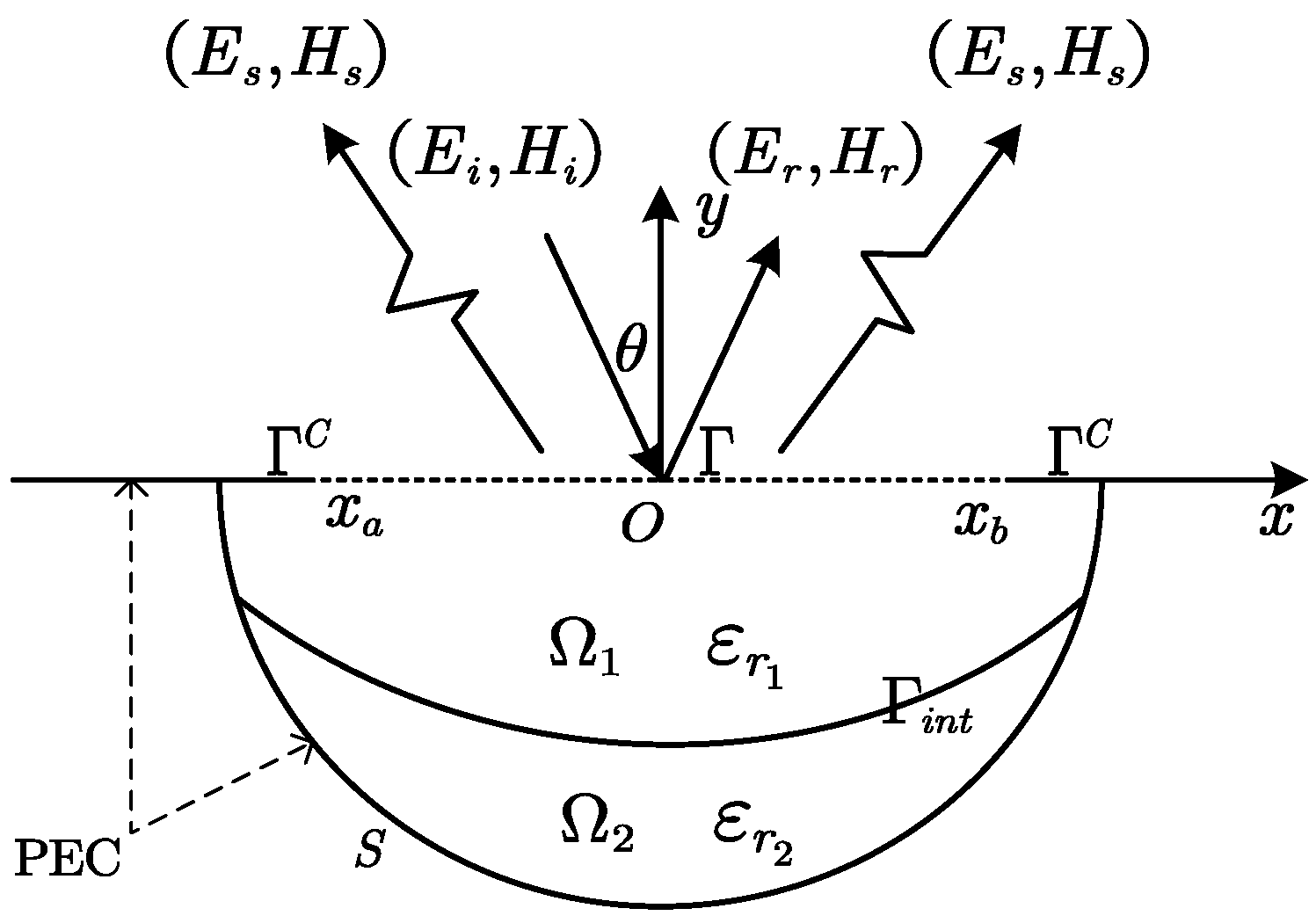
2. The Mathematical Model of a Partly Covered Groove

We investigate the scattering of a partly covered groove injected by the indent wave with an incident angle of $\theta$, embedded in the half plane of a perfect electric conductor, as shown in Figure 1. $(E_i,H_i)$ is the incident electric field and the magnetic field. $E_r,H_r$ and $E_s,H_s$ express the reflected field and the scattered field, respectively. The groove domain is divided into two subdomains, ${\Omega }_1$ and ${\Omega }_2$. Let ${\epsilon }_{r_1}$ be the relative permittivity of the medium filling in ${\Omega }_1$. Similarly, ${\epsilon }_{r_2}$ is the relative permittivity of another medium. The permeability of non-magnetic media filling in the whole groove $\Omega$ and the half plane ${\mathbb{R}}_{+}^2=\left\{(x,y)\in R^2:y>0\right\}$ is set to the permeability $u_0=4\pi \times {10}^{-7}H/m$ of the free space. The interface between the two media is denoted as ${\Gamma }_{int}$. Let $\Gamma$ be the aperture of the partly covered groove, whose endpoints are $x_a$ and $x_b$. ${\Gamma }^C=\{y=0\}\setminus \Gamma$ and the boundary S are the surface of the perfect electric conductor.

According to the differential form of time-harmonic Maxwell equations without source, we have the following formulation for electric field

$$\nabla \times \nabla \times \mathbf{E}-k_0^2{\epsilon }_r\mathbf{E}=0,$$

where

$${\epsilon }_r=\left\{\begin{array}{cc}\hfill {\epsilon }_{r_1}\hfill & \hfill \mathrm{in}{\Omega }_1,\hfill \\ \hfill {\epsilon }_{r_2}\hfill & \hfill \mathrm{in}{\Omega }_2,\hfill \\ \hfill 1\hfill & \hfill \mathrm{in}{\mathbb{R}}_{+}^2,\hfill \end{array}\right.$$

and the total electric field $\mathbf{E}$ is a vector field in three dimensions. $k_0$ is the wave number of free space. For the simplicity of presentation, it is usually assumed that the groove structure, media and electromagnetic field do not change with the z axis, resulting in two polarization modes: transverse magnetic (TM) and transverse electric (TE). In this paper, we focus on TM polarization, where the electric field has only a third component, that is, the indent electric field $E_i=(0,0,u_i)$. We assume $u_i=e^{\mathrm{i}{k}_0(xcos\theta -ysin\theta )}$, and then $u_r=-e^{\mathrm{i}{k}_0(xcos\theta +ysin\theta )}$ denotes the z component of the reflected field. The Helmholtz equation of the scattering problem is as follows

$$\begin{array}{ll}\Delta u+k_0^2{\epsilon }_{r}u=0& \mathrm{in}\Omega \cup {\mathbb{R}}_{+}^2,\\ u=0& \mathrm{on}{\Gamma }^C\cup S,\end{array}$$

(1)

where $u=u_i+u_r+u_s$ is the z component of the total field and $u_s$ is the z component of the scattered field.

By means of Green’s function in the upper half plane, we can obtain the non-local boundary condition on the aperture of the partly covered groove. The unbounded scattering is reduced into the internal problem of the groove. The scattered field of the upper half plane satisfies the following governing equations

$$\begin{array}{ll}\Delta u_s+k_0^2{u}_s=0& \mathrm{in}{\mathbb{R}}_{+}^2,\\ u_s=0& \mathrm{on}{\Gamma }^C,\\ u_s=u& \mathrm{on}\Gamma .\end{array}$$

(2)

Recall that Green’s function with Dirichlet boundary conditions in the upper half plane is given by

$$\begin{array}{ll}{\Delta }_{{\mathbf{x}}^{\prime }}{G}_d(\mathbf{x},{\mathbf{x}}^{\prime })+k_0^2{G}_d(\mathbf{x},{\mathbf{x}}^{\prime })=-{\delta }_{\mathbf{x}}\left({\mathbf{x}}^{\prime }\right)& \hfill \mathrm{in}{\mathbb{R}}_{+}^2,\hfill \\ G_d(\mathbf{x},{\mathbf{x}}^{\prime })=0& \mathrm{on}{y}^{\prime }=0,\end{array}$$

(3)

where $\mathbf{x}=(x,y)$ is the fixed source point and ${\mathbf{x}}^{\prime }=(x^{\prime },y^{\prime })$ is the field point. The solution of the above equations is

$$G_d(\mathbf{x},{\mathbf{x}}^{\prime })=\frac{\mathrm{i}}{4}\left[H_0^{\left(1\right)}(k_0|{\mathbf{x}}^{\prime }-\mathbf{x}\left|\right)-H_0^{\left(1\right)}(k_0|{\mathbf{x}}^{\prime }-\overline{\mathbf{x}}\left|\right)\right],$$

(4)

where $\overline{\mathbf{x}}=(x,-y)$ is the mirror image of the source point $\mathbf{x}$ and $H_0^{\left(1\right)}\left(z\right)$ expresses the first Hankel function of zero order.

Multiplying both sides of the first formula of (2) by $G_d$ and integrating with respect to ${\mathbf{x}}^{\prime }$ in the upper half plane ${\mathbb{R}}_{+}^2$, we have

$${\int }_{{\mathbb{R}}_{+}^2}\left(G_d·\Delta u_s+k_0^2{G}_d·u_s\right)d{\mathbf{x}}^{\prime }=0.$$

(5)

Similarly, we multiply the two sides of the first formula of (3) by $u_s$ and integrate with respect to ${\mathbf{x}}^{\prime }$ in the upper half plane. Considering the properties of Dirac function, we obtain

$${\int }_{{\mathbb{R}}_{+}^2}\left(u_s·\Delta G_d+k_0^2{u}_s·G_d\right)d{\mathbf{x}}^{\prime }=-u_s\left(\mathbf{x}\right).$$

(6)

Subtracting (6) by (5), applying the second theorem of Green’s function and combining the Sommerfeld radiation condition

$$\underset{r\to \infty }{lim}\sqrt{r}\left(\frac{\partial u_s}{\partial r}-\mathrm{i}{k}_0{u}_s\right)=0,\underset{r\to \infty }{lim}\sqrt{r}\left(\frac{\partial G_d}{\partial r}-\mathrm{i}{k}_0{G}_d\right)=0,$$

(7)

we finally obtain the boundary integral expression of the scattered field

$$u_s\left(\mathbf{x}\right)={\int }_{\Gamma }\frac{\partial G_d(\mathbf{x},{\mathbf{x}}^{\prime })}{\partial y^{\prime }}{u}_s\left({\mathbf{x}}^{\prime }\right)d{\mathbf{x}}^{\prime }\mathrm{in}{\mathbb{R}}_{+}^2,$$

(8)

where

$$\frac{\partial G_d(\mathbf{x},{\mathbf{x}}^{\prime })}{\partial y^{\prime }}{|}_{y^{\prime }=0}=\frac{\mathrm{i}{k}_{0}y}{2r}{H}_1^{\left(1\right)}\left(k_{0}r\right).$$

(9)

Here, $r=\sqrt{{(x-x^{\prime })}^2+y^2}$ and $H_1^{\left(1\right)}\left(z\right)$ is the first Hankel function of first order. Taking the partial derivative of (8) with respect to y gives

$${\left.\frac{\partial u_s\left(\mathbf{x}\right)}{\partial y}\right|}_{y=0^{+}}=\frac{\mathrm{i}{k}_0}{2}{\int }_{\Gamma }\frac{1}{|x-x^{\prime }|}{H}_1^{\left(1\right)}\left(k_0|x-x^{\prime }|\right)u_s\left(x^{\prime },0\right)d{x}^{\prime }\mathrm{on}\Gamma .$$

(10)

Substituting $u_s=u-u_i-u_r$ into (10) gives rise to

$${\left.\frac{\partial u\left(\mathbf{x}\right)}{\partial y}\right|}_{y=0^{+}}=\frac{\mathrm{i}{k}_0}{2}{\int }_{\Gamma }\frac{1}{|x-x^{\prime }|}{H}_1^{\left(1\right)}\left(k_0|x-x^{\prime }|\right)u\left(x^{\prime },0\right)d{x}^{\prime }-2\mathrm{i}\beta e^{\mathrm{i}\alpha x}\mathrm{on}\Gamma ,$$

(11)

where $\alpha =k_{0}cos\theta$ and $\beta =k_{0}sin\theta$. According to the electric field continuity condition

$$\frac{\partial u}{\partial n}{|}_{y=0^{+}}=\frac{1}{{\mu }_r}\frac{\partial u}{\partial n}{|}_{y=0^{-}},$$

(12)

where n represents the unit normal vector at the aperture pointing to the upper half plane and ${\mu }_r=1$ is the relative permeability, (11) can be rewritten as

$$\frac{\partial u\left(\mathbf{x}\right)}{\partial n}=\frac{\mathrm{i}{k}_0}{2}{\int }_{\Gamma }\frac{1}{|x-x^{\prime }|}{H}_1^{\left(1\right)}\left(k_0|x-x^{\prime }|\right)u\left(x^{\prime },0\right)d{x}^{\prime }-2\mathrm{i}\beta e^{\mathrm{i}\alpha x}\mathrm{on}\Gamma .$$

(13)

This is called the non-local boundary condition on the aperture of the partly covered groove. It follows that

$$\begin{array}{cc}\Delta u+k_0^2{\epsilon }_{r}u=0\hfill & \hfill \mathrm{in}\Omega ,\\ u=0\hfill & \hfill \mathrm{on}\partial \Omega \setminus \Gamma ,\\ \frac{\partial u}{\partial n}=\mathcal{I}\left(u\right)+g\left(x\right)\hfill & \hfill \mathrm{on}\Gamma .\end{array}$$

(14)

Here, $g\left(x\right)=-2\mathrm{i}\beta e^{\mathrm{i}\alpha x}.$$\mathcal{I}\left(u\right)=\frac{\mathrm{i}{k}_0}{2}{\int }_{\Gamma }\frac{1}{|x-x^{\prime }|}{H}_1^{\left(1\right)}\left(k_0|x-x^{\prime }|\right)u\left(x^{\prime },0\right)d{x}^{\prime }$, which includes the approximation of the Hadamard integral, as shown in [22].

3. Weak Form of the Scattering Problem

In this section, we derive the weak form of (14) in detail. The function space of the solutions satisfies the squared quadratic property of the solutions and their derivative. The Sobolev space ${\mathrm{H}}^1$ is used,

$${\mathrm{H}}^1(\Omega )=\left\{u\in L^2{(\Omega ):\left|\right|u\left|\right|}_{L^2}^2+{\left|\right|\nabla u\left|\right|}_{L^2}^2<\infty \right\},$$

with its norm

$${\left|\right|u\left|\right|}_{{\mathrm{H}}^1(\Omega )}={\left({\int }_{\Omega }(u^2+\nabla u·\nabla u)dxdy\right)}^{\frac{1}{2}}.$$

On account of the boundary operator on the aperture, we define the trace functional space

$${\mathrm{H}}^{\frac{1}{2}}(\Gamma )=\left\{u:u\in L^2(\Gamma ),{\int }_{\Gamma }{\left(1+{\xi }^2\right)}^{\frac{1}{2}}{\left|\widehat{u}\right|}^{2}d\xi <\infty \right\},$$

with its norm

$${\left|\right|u\left|\right|}_{{\mathrm{H}}^{\frac{1}{2}}(\Gamma )}={\left({\int }_{\Gamma }{\left(1+{\xi }^2\right)}^{\frac{1}{2}}{\left|\widehat{u}\right|}^{2}d\xi \right)}^{\frac{1}{2}}.$$

Here, $\widehat{u}\left(\xi \right)={\int }_{\Gamma }u\left(x\right)e^{ix\xi }dx$ is the Fourier transformation of u. Additionally, the test function space is denoted as

$${\mathrm{H}}_0^1(\Omega )=\left\{v\in {\mathrm{H}}^1(\Omega ):v=0\mathrm{on}\partial \Omega \setminus \Gamma \right\}.$$

The variational formula of (14) can be obtained by multiplying the test function v on both sides and applying the partial integral method,

$${\int }_{\Omega }\left(\nabla u·\nabla v-k_0^2{\epsilon }_{r}uv\right)dxdy-{\int }_{\Gamma }\mathcal{I}\left(u\right)vdx={\int }_{\Gamma }gvdx.$$

(15)

Find $u\in {\mathrm{H}}^1(\Omega )$, such that

$$a(u,v)=b\left(v\right),\forall v\in {\mathrm{H}}_0^1(\Omega ),$$

(16)

where $a(u,v)={\int }_{\Omega }\left(\nabla u·\nabla v-k_0^2{\epsilon }_{r}uv\right)dxdy-{\int }_{\Gamma }\mathcal{I}\left(u\right)vdx$, and $b\left(v\right)={\int }_{\Gamma }gvdx$.

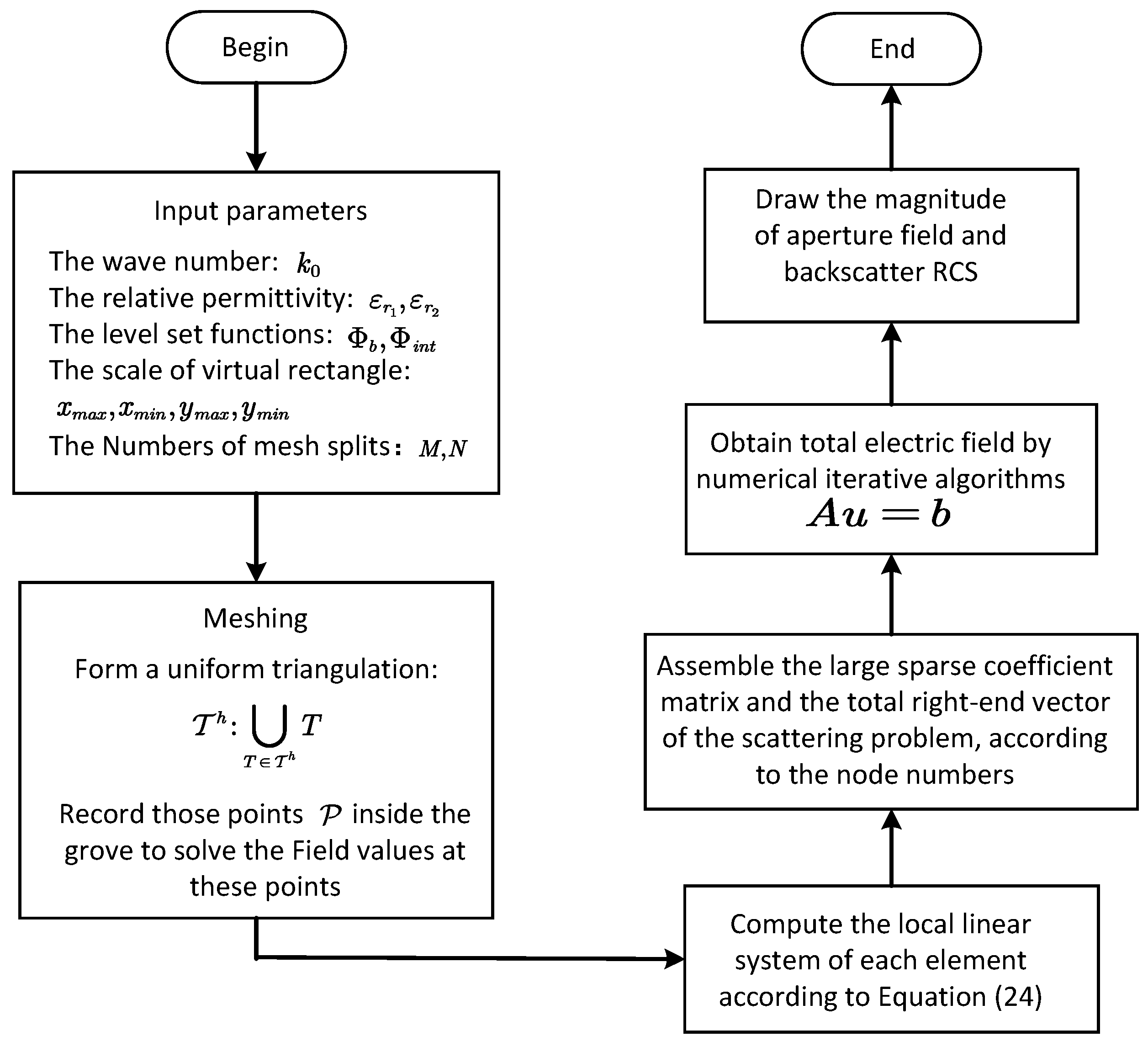
4. Non-Traditional Finite Element Method

In this section, we present the non-traditional finite element method by means of non-body-fitted uniform meshes and explain how to transfer the jump conditions of the interface to the split elements.

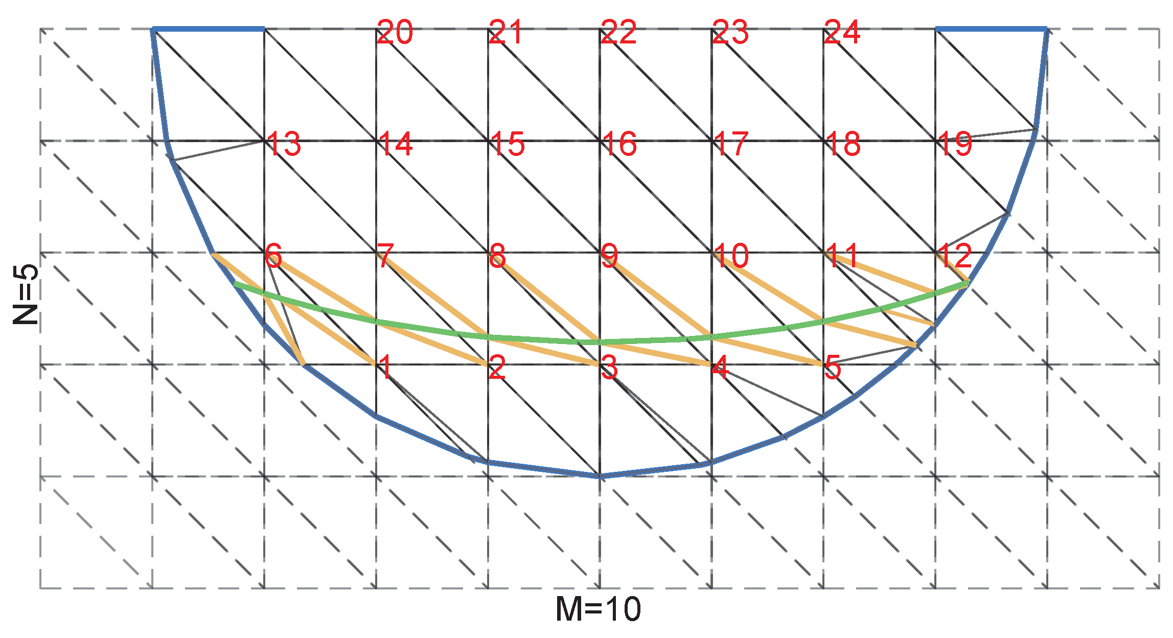
4.1. Non-Body-Fitted Mesh Generation

First, we need to build a virtual rectangle with the top edge flush with the aperture of the partly covered groove and slightly larger than the groove. The virtual rectangle is divided into M parts transversely and N parts vertically, and the step sizes are $h_x=\frac{x_{max}-x_{min}}{M}$ and $h_y=\frac{y_{max}-y_{min}}{N}$, respectively. Then, the grid size is $h=max\left\{h_x,h_y\right\}$ and the collection of Cartesian grid points is $\left\{(x_i,y_j):x_i=x_{min}+i{h}_x,i=0,1,\cdots ,M;\right.$ $\left.y_j=y_{min}+j{h}_y,j=0,1,\cdots ,N\right\}$. Each regular rectangular element is divided along its main diagonal into a lower triangle and an upper triangle, with the vertex coordinates of the lower triangle being $(x_{i-1},y_{j-1}),(x_i,y_{j-1})$, and $(x_{i-1},y_j)$, and the vertex coordinates of the upper triangle being $(x_i,y_j),(x_{i-1},y_j)$, and $(x_i,y_{j-1}),i=1,2,\cdots ,M,j=1,2,\cdots ,N$. Finally, all triangles are collected to form a uniform triangulation ${\mathcal{T}}_h=\sum _{T\in {\mathcal{T}}_h}T.$

We consider the semicircular partly covered groove as an example for a detailed discussion, as shown in Figure 2. The blue curve represents the groove boundary and the covered aperture, and the green curve represents the interface between different media. The yellow lines only appear when the media interface intersects with the uniform triangular element. The red markers represent the global node number, i.e., the degrees of freedom for a linear system generated by the scattering problem.

We can observe that there are two regions surrounded by dotted lines and solid lines. This blue curve plays a crucial role, which can be described by the level set function ${\Phi }_b(x,y)$. ${\Phi }_b$ is greater than zero in the domain outside the groove, which is not included in the calculation. If ${\Phi }_b=0$ at a grid point, then this point is on the boundary. ${\Phi }_b<0$ means that this point is inside the groove. In addition, the level set function of the interface is denoted by ${\Phi }_{int}(x,y)$. When the grid point is in ${\Omega }_1$, the value ${\Phi }_{int}$ is greater than 0. When this point falls in ${\Omega }_2$, ${\Phi }_{int}$ is less than 0. ${\Phi }_{int}$ is equal to 0 at the interface. It is easy to determine the region where the grid nodes are located through the level set function. Then, we only need to consider the computation in the groove, where the set of nodes is represented by $\mathcal{P}$. For the sake of follow-up, we still need to introduce two sets of grid functions

$${\mathrm{H}}^{1,h}=\left\{{\omega }^h=\left({\omega }_{i,j}\right):0\le i\le M,0\le j\le N\right\},$$

and

$${\mathrm{H}}_0^{1,h}=\left\{{\omega }^h=\left({\omega }_{i,j}\right)\in {\mathrm{H}}^{1,h}:\mathrm{if}i=0,M\mathrm{or}j=0,N\right\}.$$

Two extension operators from coefficient vectors to finite element functions are constructed. The first operator is ${\mathcal{V}}^h:{\mathrm{H}}^{1,h}\to {\mathrm{H}}_0^1(\Omega )$. For any ${\psi }^h\in {\mathrm{H}}_0^{1,h}$, ${\mathcal{V}}^h\left({\psi }^h\right)$ is a standard continuous piecewise linear function and matches ${\psi }^h$ on the grid, which serves as a basic function of a finite dimensional subspace ${\mathrm{H}}_0^{1,h}(\Omega )$ of the Sobolev space ${\mathrm{H}}_0^1(\Omega )$. Another extension operator ${\mathcal{U}}^h$ is a similar construction. It is a linear function in triangular elements that are not truncated by the boundary and interface. In those truncated elements, it consists of two pieces of linear functions, one on $T_1\subseteq {\Omega }_1$ and the other on $T_2\subseteq {\Omega }_2$. The position of the discontinuity at the interface is the straight segment ${\Gamma }_T^h$. Here, we introduce two kinds of interface conditions, the value jump condition

$$\left[u\right]{|}_{{\Gamma }_{int}}\equiv u^{\left(1\right)}-u^{\left(2\right)}=p,$$

and the flux jump condition

$$\left[c\frac{\partial u}{\partial n}\right]{|}_{{\Gamma }_{int}}\equiv c^{\left(1\right)}\frac{\partial u^{\left(1\right)}}{\partial n}-c^{\left(2\right)}\frac{\partial u^{\left(2\right)}}{\partial n}=q,$$

where $p,q$ are given functions and $c^{\left(1\right)},c^{\left(2\right)}$ are the reciprocal of the relative permeability. In the scattering problem of the partly covered groove, the electric field values and fluxes at the interface are continuous, i.e., $p=q=0$. Since the fillings are supposed to be non-magnetic, $c^{\left(1\right)}=c^{\left(2\right)}=1$.

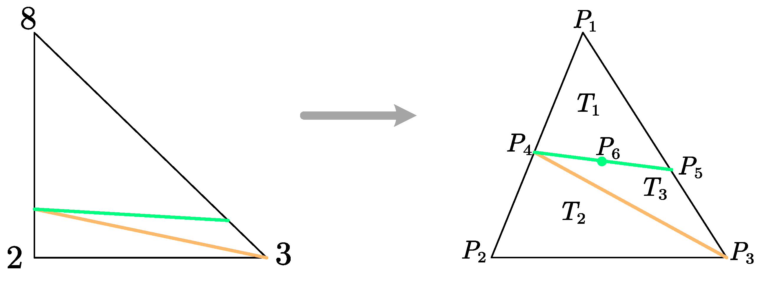
4.2. The Processing of Intersecting Elements with Interface

We consider the treatment of the triangle that intersects the media interface. Let us take a triangle with node numbers 2, 3 and 8, as shown in Figure 3. First, the nodes are renumbered. $P_4,P_5$ are the intersection points of $P_1{P}_2,P_1{P}_3$ and the interface, respectively. $P_6$ is the midpoint of $P_4{P}_5$. Let $T_1$ belongs to ${\Omega }_1$ and $T_2,T_3$ belong to ${\Omega }_2$. We consider the jumps at $P_4$ and $P_5$

$$u_4^{\left(1\right)}-u_4^{\left(2\right)}=p_4,u_5^{\left(1\right)}-u_5^{\left(2\right)}=p_5,$$

(17)

and the flux jump at $P_6$

$$c^{\left(1\right)}\frac{\partial u_6^{\left(1\right)}}{\partial n}-c^{\left(2\right)}\frac{\partial u_6^{\left(2\right)}}{\partial n}=q_6,$$

(18)

where the character superscript denotes the domain number and the subscript denotes the node number.

We know that the basic function of the solution space consists of the linear function on $T_1$ and the linear function on $T_2$ and $T_3$. There are

$${\mathcal{U}}^h(x,y)=\left\{\begin{array}{cc}{d}_{1}x+e_{1}y+f_1\hfill & \mathrm{on}{T}_1,\hfill \\ d_{2}x+e_{2}y+f_2\hfill & \mathrm{on}{T}_2\cup T_3.\hfill \end{array}\right.$$

(19)

Combined with (17), the system of linear equations on $T_1$ can be expressed as

$$\begin{array}{l}{d}_1{x}_1+e_1{y}_1+f_1=u_1,\\ d_1{x}_4+e_1{y}_4+f_1=u_4^{\left(2\right)}+p_4,\\ d_1{x}_5+e_1{y}_5+f_1=u_5^{\left(2\right)}+p_5,\end{array}$$

(20)

and the system of linear equations on $T_3$ is

$$\begin{array}{l}{d}_2{x}_2+e_2{y}_2+f_1=u_2,\\ d_2{x}_3+e_2{y}_3+f_1=u_3,\\ d_2{x}_4+e_2{y}_4+f_1=u_4^{\left(2\right)}.\end{array}$$

(21)

The gradient ${[d_1,e_1]}^{\mathrm{T}}$ solved by (20) is represented by ${\nabla }^{\left(1\right)}$, and the gradient ${[d_2,e_2]}^{\mathrm{T}}$ of (21) is denoted by ${\nabla }^{\left(2\right)}$. It follows from (18) that

$$\left[c^{\left(1\right)}{\nabla }^{\left(1\right)}·n-c^{\left(2\right)}{\nabla }^{\left(2\right)}·n\right]{|}_{(x_6,y_6)}=q_6.$$

(22)

In addition, on $T_2$

$$d_2{x}_5+e_2{y}_5+f_2=u_5^{\left(2\right)}.$$

(23)

From (20) to (23), the number of equations is equal to that of unknowns, so $u_4^{\left(1\right)},u_4^{\left(2\right)},u_5^{\left(1\right)}$ and $u_5^{\left(2\right)}$ can be uniquely expressed linearly by $u_1,u_2$ and $u_3$.

In brief, the discrete idea of the non-traditional finite element method is as follows. Finding a discrete function $u^h\in {\mathrm{H}}^{1,h}$, such that for all ${\varphi }^h\in {\mathrm{H}}_0^{1,h}$, we have

$$\begin{array}{l}{\displaystyle \sum _{T\in {\mathcal{T}}^h}}\left[{\int }_{T^1}\nabla {\mathcal{U}}^h\left(u^h\right)·\nabla \mathcal{V}\left({\varphi }^h\right)dxdy+{\int }_{T^2}\nabla {\mathcal{U}}^h\left(u^h\right)·\nabla \mathcal{V}\left({\varphi }^h\right)dxdy\right.\\ \left.+{\int }_{T_1}{k}_0^2{\epsilon }_r{\mathcal{U}}^h\left(u^h\right)\mathcal{V}\left({\varphi }^h\right)dxdy+{\int }_{T_2}{k}_0^2{\epsilon }_r{\mathcal{U}}^h\left(u^h\right)\mathcal{V}\left({\varphi }^h\right)dxdy\right]\\ -{\int }_{{\Gamma }^h}\mathcal{I}\left({\mathcal{U}}^h\left(u^h\right)\right)\mathcal{V}\left({\varphi }^h\right)dx={\displaystyle \sum _{T\in {\mathcal{T}}^h}}{\int }_{{\Gamma }_T^h}g\mathcal{V}\left({\varphi }^h\right)dx.\end{array}$$

(24)

Then, we draw the flow chart of solving the scattering problem of the partly covered groove by the non-traditional finite element method in Figure 4.

5. Numerical Examples

In this section, numerical tests are carried out to verify the accuracy and computational efficiency of the non-traditional finite element method for the scattering problem from the partly covered groove. We are concerned with the magnitude of the aperture field, the distribution of the total field in the groove and the radar cross-section (RCS), which is of great interest in the field of engineering electromagnetism. Backscatter RCS is defined as follows

$$\mathrm{Backscatter}\mathrm{RCS}\left(\theta \right)=10{log}_{10}\left(\frac{4}{k_0}\left|P\left(\theta \right)\right|\right)\mathrm{dB},$$

where $\theta$ is the observation angle and the incident angle. $\left|P\right(\theta \left)\right|$ is the far-field coefficient,

$$P\left(\theta \right)=\frac{k_0}{2}sin\theta {\int }_{\Gamma }u{e}^{\mathrm{i}{k}_{0}xcos\theta }dx.$$

5.1. Example 1

We consider a square groove with an uncovered aperture, filled with layered media, that is, ${\epsilon }_{r_1}=1,{\epsilon }_{r_2}=1+4\mathrm{i}$. We suppose that the exact solution is

$$u(x,y)=\left\{\begin{array}{cc}\hfill \frac{3}{2}sin\left(\pi x\right)sin\left(\frac{\pi (y+1)}{2}\right),\hfill & \hfill (x,y)\in [0,1]\times [-0.5,0]\left({\Omega }_1\right),\hfill \\ \hfill sin\left(\pi x\right)sin\left(\frac{\pi (y+1)}{2}\right),\hfill & \hfill (x,y)\in [0,1]\times [-1,-0.5]\left({\Omega }_2\right).\hfill \end{array}\right.$$

Jump conditions on the interface can be calculated

$$\begin{array}{l}\left[u\right]{|}_{{\Gamma }_{int}}=\frac{1}{2}sin\left(\pi x\right)sin\left(\frac{\pi (y+1)}{2}\right),\\ \left[\frac{\partial u}{\partial n}\right]{|}_{{\Gamma }_{int}}={\left[\frac{\pi }{2}cos\left(\pi x\right)sin\left(\frac{\pi (y+1)}{2}\right),\frac{\pi }{4}sin\left(\pi x\right)cos\left(\frac{\pi (y+1)}{2}\right)\right]}^T,\end{array}$$

and the source term can also be calculated

$$f(x,y)=\left\{\begin{array}{ll}\frac{3}{2}(k_0^2{\epsilon }_{r_1}-\frac{5}{4}{\pi }^2)sin\left(\pi x\right)sin\left(\frac{\pi (y+1)}{2}\right)& \mathrm{in}{\Omega }_1,\\ \hfill (k_0^2{\epsilon }_{r_2}-\frac{5}{4}{\pi }^2)sin\left(\pi x\right)sin\left(\frac{\pi (y+1)}{2}\right)\hfill & \hfill \mathrm{in}{\Omega }_2.\hfill \end{array}\right.$$

The wave number is $k_0=2\pi$, and the square groove is divided into $20\times 20$. Figure 5 shows the exact solution, and Figure 6 shows the numerical solutions obtained by the non-traditional and traditional finite element method. Obviously, the numerical solution obtained by the non-traditional finite element method is closer to the exact solution. We give the error and convergence rate at $L^2$ norm after grid encryption in

Table 1. Error and convergence rate with ${\epsilon }_{r_1}=1,{\epsilon }_{r_2}=1+4\mathrm{i}$ and $k_0=2\pi$.

Method	Meshes	${\mathit{L}}^2$ Error	Order
	20 × 20	0.0536	–
Non-traditional	40 × 40	0.0136	1.9796
finite element	80 × 80	0.0034	1.9823
method	160 × 160	0.0009	1.9820
	20 × 20	1.7569	–
Traditional finite	40 × 40	1.6787	0.0657
element method	80 × 80	1.6398	0.0339
	160 × 160	1.6204	0.0172

. It is easily observed that our method can deal with the discontinuous interface well. The traditional approach cannot solve such problems well, which means it cannot achieve a relatively good convergence rate.

5.2. Example 2

We next consider partly covered rectangular grooves with different kinds of apertures in Figure 7, which both are 1 m wide and 0.25 m deep. In the left picture, the aperture is covered by 0.125 m at both ends, while the aperture is covered by 0.25 m in the right picture.

First of all, we assume that the groove in the left picture of Figure 7 is empty, i.e., ${\epsilon }_r=1$, and the wave number is $8\pi$. It is apparent from Figure 8 that the results calculated by our method are in good agreement with Zhao’s in [3], which shows that the non-traditional finite element method can efficiently solve the groove scattering problem. Additionally,

Table 2. Error and convergence rate with $k_0=8\pi ,{\epsilon }_r=1$.

Meshes	${\mathit{L}}^{\mathit{\infty }}$ Error	Order	${\mathit{L}}^2$ Error	Order
192 × 48	0.0359	–	0.1971	–
384 × 96	0.0094	1.9308	0.0543	1.8597
768 × 192	0.0022	2.1025	0.0144	1.9176

shows that our method still has a second-order convergence rate at $L^{\infty }$ norm and $L^2$ norm when the wave number is relatively high, which is similar to the conclusion in Example 1.

Then, we consider the electromagnetic scattering by the right groove in Figure 7. When the wave number is $2\pi$, Figure 9 and Figure 10 plot the magnitude of the aperture field at vertical incidence and the RCS corresponding to ${\epsilon }_r=1$ and $4+1\mathrm{i}$, respectively. Compared with Du’s results in [6], numerical results produced by our method agree with his, which once again confirms the accuracy of the non-traditional finite element method.

5.3. Example 3

We design a short backfire antenna model, a rectangle similar to the one in Example 2, as shown in Figure 11, which is covered by 0.6 m at the center of the aperture.

Figure 12 and Figure 13 give the magnitude of the aperture field at the normal incidence and RCS of the antenna model filled with different homogeneous media, ${\epsilon }_r=1\mathrm{or}1+4\mathrm{i}$, respectively, when the wave number is $16\pi$. We see that our method can handle the situation of covering the center of the aperture well. The magnitude and RCS are reduced to a certain extent when the relative permittivity is complex.

5.4. Example 4

We further consider an asymmetric groove that is 1 m wide and 0.5 m deep, as shown in Figure 14, where the function of the lower edge of the groove is $y=-0.25sin\left(2\pi x\right)-0.5$.

Let the wave number be $4\pi$, the magnitude of the aperture field at the normal incidence and RCS of the asymmetric groove with ${\epsilon }_r=1\mathrm{and}4+1\mathrm{i}$ are presented by Figure 15 and Figure 16. Combing Figure 14, we can conclude that the asymmetry of the magnitude plot is justified due to the asymmetry of the groove. The backscatter RCS and the magnitude of the aperture field from the groove filled with a medium with a complex permittivity are both reduced greatly, similar to Example 3.

5.5. Example 5

A semicircular groove filled with two media is considered in Figure 17. The radius of the semicircular groove is 0.5 m, and the two ends of its aperture are covered by 0.125 m. The level set function of the interface is ${\Phi }_{int}(x,y)=1-\frac{x^2}{0.7^2}-\frac{y^2}{0.{35}^2}$.

We consider that ${\Omega }_2$ is filled with different kinds of absorbing materials, setting two sets of parameters, Type 1: ${\epsilon }_{r_1}=4+1\mathrm{i},{\epsilon }_{r_2}=16.01+0.9\mathrm{i},k_0=2\pi ,8\pi$; Type 2: ${\epsilon }_{r_1}=1+0.2\mathrm{i},{\epsilon }_{r_2}=29.78+2.31\mathrm{i},k_0=2\pi ,8\pi$. We pay attention to the distribution of the total field inside the groove when the incident angle is 0. Figure 18 and Figure 19 show the distribution of the total field with Type 1 and Type 2, respectively. The magnitude of the total field in ${\Omega }_2$ is smaller than the one in ${\Omega }_1$, and the magnitude under the circumstance of high-frequency incident waves is smaller than the one under the circumstance of low-frequency incident waves. The absorbing materials have good absorption performance, and the higher the frequency, the faster the energy decays.

6. Conclusions

This paper investigates the electromagnetic scattering problem of the partly covered groove by using a new non-traditional finite element method, which can accurately solve the scattering from the groove filled with multiple media, with an irregular boundary and interface. In addition, no matter where the aperture is covered, our method can solve it well. Whether the groove is symmetrical or not does not affect the solution of our program. In the non-traditional finite element method, the generation technology of non-body-fitted mesh is more popular with engineers than producing body-fitted mesh, thanks to its simplicity and cost-saving. Additionally, this idea of uniform meshing, including determining the intersection by level set functions and transferring the interface conditions to the split elements, can also be extended to three-dimensional groove scattering or other interface problems.

References

1. Bao, G.; Sun, W.W. A fast algorithm for the electromagnetic scattering from a large cavity. SIAM J. Sci. Comput. 2005, 27, 553–574. [Google Scholar] [CrossRef]
2. Wang, Y.X.; Du, K.; Sun, W.W. A second-order method for the electromagnetic scattering from a large cavity. Numer. Math. Theory Methods Appl. 2008, 1, 357–382. [Google Scholar]
3. Zhao, M.L.; Zhu, N.; Wang, L.Q. Fast algorithms for the electromagnetic scattering by partly covered cavities. Appl. Math. Comput. 2021, 40, 7. [Google Scholar] [CrossRef]
4. Zhao, M.L.; Zhu, N. A fast preconditioned iterative method for the electromagnetic scattering by multiple cavities with high wave numbers. J. Comput. Phys. 2019, 398, 108826. [Google Scholar] [CrossRef]
5. Singer, I.; Turkel, E. High-order finite difference methods for the Helmholtz equation. Comput. Methods Appl. Mech. Eng. 1998, 163, 343–358. [Google Scholar] [CrossRef]
6. Du, K.; Sun, W.W. Numerical solution of electromagnetic scattering from a large partly covered cavity. J. Comput. Appl. Math. 2011, 235, 3791–3806. [Google Scholar] [CrossRef]
7. Zhao, M.L.; Qiao, Z.H.; Tang, T. A fast high order method for electromagnetic scattering by large open cavities. J. Comput. Math. 2011, 29, 287–304. [Google Scholar] [CrossRef]
8. Jin, J.M.; Volakis, J.L. A finite-element-boundary integral formulation for scattering by three-dimensional cavity-backed apertures. IEEE Trans. Antennas Propag. 1991, 39, 97–104. [Google Scholar] [CrossRef]
9. Jin, J.M. The Finite Element Method in Electromagnetics, 2nd ed.; John Wiley Sons: New York, NY, USA, 2002; pp. 192–206. [Google Scholar]
10. Van, T.; Wood, A.H. A time-domain finite element method for Helmholtz Equations. J. Comput. Phys. 2002, 183, 486–507. [Google Scholar] [CrossRef]
11. Du, K. Two transparent boundary conditions for the electromagnetic scattering from two-dimensional overfilled cavities. J. Comput. Phys. 2011, 230, 5822–5835. [Google Scholar] [CrossRef]
12. Huang, J.Q.; Wood, A.H.; Havrilla, M.J. A hybrid finite element-Laplace transform method for the analysis of transient electromagnetic scattering by an over-filled cavity in the ground plane. Commun. Comput. Phys. 2009, 5, 126–141. [Google Scholar]
13. Wang, J.X.; Zhang, Z.M. A hybridizable weak Galerkin method for the Helmholtz equation with large wave number: hp Analysis. Int. J. Numer. Anal. Model. 2017, 14, 744–761. [Google Scholar]
14. Xiang, Z.G.; Chia, T. A hybrid BEM/WTM approach for analysis of the EM scattering from large open-ended cavities. IEEE Trans. Antennas Propag. 2001, 49, 165–173. [Google Scholar] [CrossRef]
15. Lee, J.W.; Liu, L.W.; Hong, H.K.; Chen, J.T. Applications of the Clifford algebra valued boundary element method to electromagnetic scattering problems. Eng. Anal. Bound. Elem. 2016, 71, 140–150. [Google Scholar] [CrossRef]
16. Simpson, R.N.; Liu, Z.; Vázquez, R.; Evans, J.A. An isogeometric boundary element method for electromagnetic scattering with compatible B-spline discretizations. J. Comput. Phys. 2018, 362, 264–289. [Google Scholar] [CrossRef]
17. Takahashi, T. A fast time-domain boundary element method for three-dimensional electromagnetic scattering problems. J. Comput. Phys. 2023, 482, 112053. [Google Scholar] [CrossRef]
18. Liu, J.; Ma, F.M. A PML method for electromagnetic scattering from two-dimensional overfilled cavities. Commun. Math. Res. 2009, 25, 53–68. [Google Scholar]
19. Tang, J.W.; Paulsen, K.D.; Haider, S.A. Perfectly matched layer mesh terminations for nodal-based finite-element methods in electromagnetic scattering. IEEE Trans. Antennas Propag. 1998, 46, 507–516. [Google Scholar] [CrossRef]
20. Banks, H.T.; Browning, B.L. Time domain electromagnetic scattering using finite elements and perfectly matched layers. Comput. Methods Appl. Mech. Eng. 2005, 194, 149–168. [Google Scholar] [CrossRef]
21. Wu, X.M.; Zheng, W.Y. An adaptive perfectly matched layer method for multiple cavity scattering problems. Commun. Comput. Phys. 2016, 19, 534–558. [Google Scholar] [CrossRef]
22. Wu, J.M.; Wang, Y.X.; Li, W.; Sun, W.W. Toeplitz-type approximations to the Hadamard integral operator and their applications to electromagnetic cavity problems. Appl. Numer. Math. 2008, 58, 101–121. [Google Scholar] [CrossRef]
Figure 1. The geometry of the partly covered groove.
Mathematics 12 00254 g001
Figure 2. Sample grid generation with M = 10 , N = 5 .
Mathematics 12 00254 g002
Figure 3. Intersection element generalization.
Mathematics 12 00254 g003
Figure 4. Flow chart of the non-traditional finite element method for solving the scattering problem of the partly covered groove.
Mathematics 12 00254 g004
Figure 5. Exact solution with ε r 1 = 1 , ε r 2 = 1 + 4 i and k 0 = 2 π .
Mathematics 12 00254 g005
Figure 6. Numerical solutions by the non-traditional finite element method (left) and traditional finite element method (right) with ε r 1 = 1 , ε r 2 = 1 + 4 i and k 0 = 2 π .
Mathematics 12 00254 g006
Figure 7. Partly covered rectangular grooves with different kinds of apertures.
Mathematics 12 00254 g007
Figure 8. The magnitude of the aperture field at the normal incidence of the groove in the left picture with k 0 = 8 π , ε r = 1 .
Mathematics 12 00254 g008
Figure 9. The magnitude of the aperture field (left) at θ = 0 and RCS (right) for the groove in the right picture filled with ε r = 1 and with k 0 = 2 π .
Mathematics 12 00254 g009
Figure 10. The magnitude of the aperture field (left) at θ = 0 and RCS (right) for the groove in the right picture filled with ε r = 4 + 1 i and with k 0 = 2 π .
Mathematics 12 00254 g010
Figure 11. A short backfire antenna model.
Mathematics 12 00254 g011
Figure 12. The magnitude of the aperture field (left) at θ = 0 and RCS (right) for the short antenna model filled with ε r = 1 and with k 0 = 16 π .
Mathematics 12 00254 g012
Figure 13. The magnitude of the aperture field (left) at θ = 0 and RCS (right) for the short antenna model filled with ε r = 1 + 4 i and with k 0 = 16 π .
Mathematics 12 00254 g013
Figure 14. An asymmetric groove.
Mathematics 12 00254 g014
Figure 15. The magnitude of the aperture field (left) at θ = 0 and RCS (right) for the asymmetric groove filled with ε r = 1 and with k 0 = 4 π .
Mathematics 12 00254 g015
Figure 16. The magnitude of the aperture field (left) at θ = 0 and RCS (right) for the asymmetric groove filled with ε r = 4 + 1 i and with k 0 = 4 π .
Mathematics 12 00254 g016
Figure 17. A partly covered semicircular groove with a radius of 0.5 m.
Mathematics 12 00254 g017
Figure 18. The distribution of the magnitude of the total field with Type 1 ( k 0 = 2 π (left), k 0 = 8 π (right)).
Mathematics 12 00254 g018
Figure 19. The distribution of the magnitude of the total field with Type 2 ( k 0 = 2 π (left), k 0 = 8 π (right)).
Mathematics 12 00254 g019