An Advanced Segmentation Approach to Piecewise Regression Models

Abstract

Two problems concerning detecting change-points in linear regression models are considered. One involves discontinuous jumps in a regression model and the other involves regression lines connected at unknown places. Significant literature has been developed for estimating piecewise regression models because of their broad range of applications. The segmented (SEG) regression method with an R package has been employed by many researchers since it is easy to use, converges fast, and produces sufficient estimates. The SEG method allows for multiple change-points but is restricted to continuous models. Such a restriction really limits the practical applications of SEG when it comes to discontinuous jumps encountered in real change-point problems very often. In this paper, we propose a piecewise regression model, allowing for discontinuous jumps, connected lines, or the occurrences of jumps and connected change-points in a single model. The proposed segmentation approach can derive the estimates of jump points, connected change-points, and regression parameters simultaneously, allowing for multiple change-points. The initializations of the proposed algorithm and the decision on the number of segments are discussed. Experimental results and comparisons demonstrate the effectiveness and superiority of the proposed method. Several real examples from diverse areas illustrate the practicability of the new method.

1. Introduction

Piecewise regression models have been widely used in many practical situations where the relationship between the response and explanatory variables changes abruptly at certain points. These places are called change-points, break-points, or thresholds. Figure 1 illustrates some possible piecewise regressions between the response and generic covariate x.

In analyzing regressions with change-points, spline methods and piecewise regressions have been commonly adopted in the literature. Spline regressions are mainly used to approximate smooth regression functions. A spline function (q-spline) is a piecewise polynomial of degree q with q − 1 continuous derivatives at the change-point (c.f. [1]). The change-points are called knots in spline regressions. Seber [1] commented that regression splines are appropriate when one aims at finding the best fitted model to utilize in prediction or in finding extreme values of the regression curve. More applications and discussion on spline methods can be found in references [1,2,3]. The emphasis of regression spline is on modelling smooth regression relationships rather than illustrating structural changes in the regression relations (c.f. [1]). Thus, the regression coefficients resulted from splines may not measure the effect on the response and the estimated parameters are not explicitly interpretable (c.f. [4]).

By contrast, piecewise regression analyses focus on addressing the tendency relationships between response and explanatory variables, as indicated by abrupt changes between well-mannered regimes [1]. Therefore, locating change-points and obtaining adequate and meaningful estimates of parameters are the primary purpose for fitting piecewise regression models. The estimations for change-points and regression coefficients are important in piecewise regressions because they are often the sign for knowing when and how the trend of data changes. This information is critical to decision making. Change-point detection has been identified as a challenging problem for modern, big data applications [5].

Multiphase models provide a simple and interpretable way to deal with non-linear problems and provide meaningful regression parameters. Therefore, researchers have advocated piecewise regression models as better alternatives to solve regression problems which involve unknow change-points. This paper aims at dealing with regression problems involving abrupt changes, with continuous or discontinuous jumps at unknown places. This approach involves piecewise regression analyses.

Change-point regression problems occur in many fields such as molecular biology, medicine, climatology, engineering, and econometrics [4,6,7,8]. In medical science, segmented regression models are employed to see whether the effect of some risk factor on the response alters abruptly. For example, the risk of cancer is low for young people, but the risk rises quickly for people of age beyond a certain age threshold [9]. In the oil and gas industry, sequential well-log data often appear as abrupt jumps at the transitions of rock strata. Each change-point in the well-log sequence indicates that a new rock type is encountered. Thus, change-point detection is crucial in oil-drilling. An example of well-log data from [10] was analyzed via many different change-point methods [5,11,12,13]. Figure 2a displays data plots of the indexed measurements from 2000 to 2650 in the well-log data set and discloses five discontinuous jumps in the data series. Moreover, piecewise regressions are also serviceable for clustering objects into groups based on a certain explanatory variable. For instance, one may want to classify cars based on the relationship between fuel efficiency (measured by miles per gallon, denoted by MPG), weights (WTs), and horsepower (HP). The graph of a data set taken from [8] shows a discontinuous and nonlinear relationship between MPG and WT (see Figure 2b).

This paper is presented as follows. Section 2 presents the literature review. Section 3 describes Muggeo’s segmented method and proposes an advanced segmentation approach for piecewise regression models free of the continuity restriction. The IJD method is introduced for choosing proper initial values. Section 4 provides experimental examples and comparisons to demonstrate the effectiveness and superiority of the proposed method. Severa real data sets are used to illustrate the practicability of the new approach. Finally, Section 5 provides concluding remarks.

2. Literature Review

Change-point problems, first introduced in the quality control context, have developed into a fundamental issues in many areas. Numerous methodologies have been introduced for solving change-point problems. Maximum likelihood approaches, Bayesian analyses, grid-searching approaches, quantile regression, and non-parametric methods are among the approaches which have been employed to resolve change-point problems. A major difficulty in the estimations for change-point regression models is the non-smoothness of the likelihood function with respect to the change-point parameter. Many authors have tried to bypass this problem through various smooth transitions between two adjoining segments. Muggeo [4] presented a segmented (SEG) regression method thorough a linear transition to estimate change-points and the regression model. The SEG method is available for simultaneous inference on change-points and regression coefficients, but it is only feasible for connected regression models. Lu and Chang [12] (2018) adopted mixture modelling approaches to bypass the non-smooth difficulty and created two algorithms, called EM-BP and FCM-BP, to obtain estimates. These two algorithms can produce maximum likelihood estimates for change-points and regression coefficients simultaneously, but they are computationally intensive in cases of multiple change-points or large data sets due to the calculations required for each possible collection of change-points. Bayesian approaches are also considered for change-point regressions [14,15]. One concern with Bayesian analysis is the computational effort, due to a large number of iterations required in Markov chain Monte Carlo simulations.

Nonparametric methods are needed when data cannot be well approximated through parametric distributions. An efficient nonparametric maximum likelihood approach was proposed via dynamic programming (DP) [16]. Garreau and Arlot [17] proposed a nonparametric kernel change-point algorithm (KCP) to locate CPs through model selection associated with a penalized kernel criterion. Thus, the performance of KCP depends on a suitable penalty. Moreover, Frick et al. [18] introduced a simultaneous multiscale change-point estimator (SMUCE) method which does not only give the estimates of the change-point but also the confidence intervals. Pein et al. [19] further advanced SMUCE to be used for heterogeneous models. Moreover, some authors proposed a wild binary segmentation (WBS) method for improving the binary segmentation (BS) approach [20,21]. These two methods assume that regression errors are normally distributed; hence, they are not robust to atypical data. Some researchers focused on the issue of computational efficiency. Haynes et al. [22] presented an efficient algorithm to find a suitable penalty choice so that the computational cost can be reduced. Recently, the resistance of algorithms in the presence of abnormal observations has been studied [23,24,25,26]. A common aspect of these methods is the computational effort. For a review of more research on change-point issues, we refer to articles [27] and the references therein.

There are often some restrictions on the aforementioned methods. Muggeo [4] proposed a segmented regression method by using Taylor expansions to deal with change-point regressions. The segmented method is allowable for multiple change-points but restricted to continuous regression lines. Muggeo’s segmented (SEG) method is easy to implement, converges fast, and produces adequate estimators. Particularly, Muggeo [28] further introduced an R package called “segmented” to facilitate the use of the segmented regression method. The SEG method has been widely employed in a great many applications [28,29,30,31,32], especially in several recent analyses of the COVID-19 epidemic curve [33,34,35]. Because of its easiness and high efficiency, the segmented regression method was further combined with rank-based estimation to make the segmented method more resistant against outliers (c.f. [7,32]). Many researchers [7,12,32,36] recognized that the SEG method works well when the piecewise model is known to be continuous at change-points. But small deviations from continuity in the regression lines may distort the estimations made by SEG method. For real applications, continuity cannot be simply assumed when solving a change-point problem. Continuity may be very probable and reasonable for medical or biological problems, while such a supposition may not be appropriate in economics, finance, and quality control [36]. As shown in Figure 2, continuity is clearly infeasible for both well-log data and car data; hence, the segmented method is not attainable for these real problems. The restriction of continuity really limits the practical applications of the SEG method. This motivates us to develop a new method for change-point regressions, without requiring continuity limitation.

In this paper, we introduce an advanced segmented regression model to solve piecewise regression problems. We propose a segmentation procedure to fit the piecewise regression model, allowing for multiple change-points free of the continuity restriction. We further propose an intuitive jump detection (IJD) method to make the new proposed method more robust to initializations and, hence, increase the precision of estimates. The proposed method is applicable to problems in diverse areas. It is useful for areas where jumps are very likely to occur, such as applications in finance and engineering [37,38,39].

3. Methodology

3.1. Muggeo’s Segmented Regression Method

We first review Muggeo’s [4] segmented (SEG) regression method. Suppose a piecewise regression model of K segments is represented by

$$g(E(Y))=f(X)+\beta h(z;\psi )$$

where $Y$ is the response, $g(\cdot )$ represents the link function for $E(Y)$, $f(X)$ is the predictor allowing any variable with a linear parameter, and $h(z;\psi )$ is the non-linear term for the Z variable with parameter $\psi$. For simplicity, the predictor $f(X)$ will be omitted because there is no difference among regression models in the following. Thus, a segmented regression model can be represented by

$$E(Y)={\alpha }_0+{\beta }_{0}z+{\displaystyle \sum _k{\beta }_k{(z-{\psi }_k)}_{+}}$$

(1)

where $\psi ={({\psi }_1,{\psi }_2,\dots ,{\psi }_K)}^T$ are change-points and ${(z-{\psi }_k)}_{+}=(z-{\psi }_k)\times I(z>{\psi }_k)$ for $k=1,\dots ,K$. Muggeo [4] proposed to approximate the non-linear term using a first-order Taylor’s expansion around ${\psi }_k^{(0)}$:

$${(z-{\psi }_k)}_{+}\doteq {(z-{\psi }_k^{(0)})}_{+}+(\psi -{\psi }_k^{(0)})(-1)I(z>{\psi }_k^{(0)}), \mathrm{for} k=1,\dots ,K.$$

Thus, Equation (1) can be rewritten as

$$\begin{array}{cc}E(Y)& \doteq {\alpha }_0+{\beta }_{0}z+{\displaystyle \sum _k{\beta }_k{(z-{\psi }_k^{(0)})}_{+}}+{\displaystyle \sum _k{\beta }_k(\psi -{\psi }_k^{(0)})(-1)I(z>{\psi }_k^{(0)})}\hfill \\ & ={\alpha }_0+{\beta }_{0}z+{\displaystyle \sum _k{\beta }_k{U}_k^{(0)}+}{\displaystyle \sum _k{\gamma }_k{V}_k^{(0)}}\hfill \end{array}$$

(2)

where

$$U_k^{(s)}={(z-{\psi }_k^{(s)})}_{+}, V_k^{(s)}=-I(z>{\psi }_k^{(s)}), {\gamma }_k^{(s)}={\beta }_k^{(s)}({\psi }_k-{\psi }_k^{(s)}).$$

(3)

Hence, in the (s + 1)th iteration,

$${\psi }_k^{(s+1)}\doteq {\psi }_k^{(s)}+\frac{{\gamma }_k^{(s)}}{{\beta }_k^{(s)}}, \mathrm{for} k=1,\dots ,K.$$

(4)

We summarize the SEG method as follows.

Given the initial ${\psi }^{(0)}$ and stop criterion $\epsilon$, perform the following steps in the (s + 1)th iteration:

• Calculate $U^{(s)}$ and $V^{(s)}$ by (3).
• Fit the model given by (2) to derive ${\alpha }^{(s)}, {\beta }^{(s)}, {\gamma }^{(s)}$.
• Update ${\psi }_k^{(s+1)}$ by (4).
• Repeat steps 1–3 until $‖{\psi }^{(s+1)}-{\psi }^{(s)}‖<\epsilon$.

3.2. The Proposed DSR Method

3.2.1. The New Defined Piecewise Regression Model

Following the previous illustrations, Muggeo [4] introduced a segmented regression model with K change-points, as given by Equation (1). For simplicity, other predictors are omitted. Next, we propose an approach to deal with the infeasibility of SEG in detecting discontinuous jumps. The new proposed method is attainable for locating both continuous change-points and discontinuous jump points simultaneously.

Since disjoint jump points are exactly the break-points of piecewise regression models, we define a piecewise regression model allowing for the occurrence of jumps at change-points by

$$E(Y)={\alpha }_0+{\beta }_{0}z+{\displaystyle \sum _k{\alpha }_{k}I(z>{\psi }_k)}+{\displaystyle \sum _k{\beta }_k{(z-{\psi }_k)}_{+}}$$

(5)

where $\psi ={({\psi }_1,{\psi }_2,\dots ,{\psi }_K)}^T$ are change-points and ${(z-{\psi }_k)}_{+}=(z-{\psi }_k)\times I(z>{\psi }_k),$ $k=1,\dots ,K.$ Similar to Muggeo’s SEG method, the other predictors are omitted for simplicity. In accordance with the parameterization in (5), ${\alpha }_0$ and ${\beta }_0$, respectively, represent the intercept and the slope of the leftmost segment line (i.e., for $z\le {\psi }_1$), ${\alpha }_k$ is the jump of the regression line at ${\psi }_k$, and ${\beta }_k$ is the difference-in-slopes parameter between the (k + 1)th and the kth slopes. Note that ${\alpha }_k=0$ when the segmented regression model is continuous at ${\psi }_k$. Since the log-likelihood function for estimating the piecewise model given by (5) is not differentiable, with change-points regarded as parameters, estimations for model (5) cannot be solved analytically but require iterative methods. Referring to [1,4], we approximate the nonlinear term through a first-order Taylor expansion around ${\psi }_k^{(0)}$:

$${(z-{\psi }_k)}_{+}\doteq {(z-{\psi }_k^{(0)})}_{+}+(\psi -{\psi }_k^{(0)})(-1)I(z>{\psi }_k^{(0)}), \mathrm{for} k=1,\cdots ,K.$$

Thus,

$$\begin{array}{cc}E(Y)& \doteq {\alpha }_0+{\beta }_{0}z+{\displaystyle \sum _k{\alpha }_{k}I(z>{\psi }_k^{(0)})}+{\displaystyle \sum _k{\beta }_k{(z-{\psi }_k^{(0)})}_{+}}+{\displaystyle \sum _k{\beta }_k({\psi }_k-{\psi }_k^{(0)})(-1)I(z>{\psi }_k^{(0)})}\hfill \\ & ={\alpha }_0+{\beta }_{0}z+{\displaystyle \sum _k{\beta }_k{(z-{\psi }_k^{(0)})}_{+}}+{\displaystyle \sum _k[{\beta }_k({\psi }_k-{\psi }_k^{(0)})-{\alpha }_k](-1)I(z>{\psi }_k^{(0)})}\hfill \\ & ={\alpha }_0+{\beta }_{0}z+{\displaystyle \sum _k{\beta }_k{U}_k^{(0)}+}{\displaystyle \sum _k{\gamma }_k{V}_k^{(0)}}.\hfill \end{array}$$

(6)

At the (s + 1)th iteration, we define

$$U_k^{(s)}={(z-{\psi }_k^{(s)})}_{+}, V_k^{(s)}=-I(z>{\psi }_k^{(s)}),$$

(7)

$${\gamma }_k^{(s)}={\beta }_k^{(s)}({\psi }_k-{\psi }_k^{(s)})-{\alpha }_k^{(s)}, k=1,\dots ,\mathrm{K}.$$

(8)

The model given by (6) is suitable for model errors following normal distributions or heavy tailed distributions, such as t or Laplace distributions. As an illustration, we assume the model error follows a normal distribution and fit the model by the least square method as follows:

$${\left({\alpha }_0^{(s)},{\beta }_0^{(s)},{\beta }_1^{(s)},{\gamma }_1^{(s)},\dots ,{\beta }_K^{(s)},{\gamma }_K^{(s)}\right)}^T={\left(X^{T}X\right)}^{-1}{X}^{T}Y$$

(9)

where the design matrix is

$$\begin{gathered} X=\left[\begin{array}{ccccccc}1& z_1& U_{11}^{(s)}& V_{11}^{(s)}& \cdots & U_{K1}^{(s)}& V_{K1}^{(s)}\\ ⋮& ⋮& ⋮& ⋮& \ddots & ⋮& ⋮\\ 1& z_n& U_{1n}^{(s)}& V_{1n}^{(s)}& \cdots & U_{Kn}^{(s)}& V_{Kn}^{(s)}\end{array}\right],Y=\left[\begin{array}{c}{y}_1\\ ⋮\\ y_n\end{array}\right],U_{ki}^{(s)}={(z_i-{\psi }_k^{(s)})}_{+}, \\ {V}_{ki}^{(s)}=-I(z_i>{\psi }_k^{(s)}), \mathrm{for} i=1,\dots ,n, k=1,\dots ,K. \end{gathered}$$

After fitting the regression model by (9), we can derive the updated estimates ${\alpha }_0^{(s)}$, ${\beta }_0^{(s)}$, ${\beta }_k^{(s)}$, and ${\gamma }_k^{(s)}$. To update the estimates of ${\alpha }_k$ and ${\psi }_k$, we can use the Equation (8) only because these two parameters merely appear in (8). However, a single equation is not enough for solving two unknowns. This is the difficulty of Muggeo’s segmented regression model in estimating piecewise models with jumps at unknown places. This may be the reason why the SEG method requires the restriction of continuity. To solve this difficulty, we consider updating ${\psi }_k$ through Equation (8) as follows:

$${\psi }_k^{(s+1)}=\frac{{\gamma }_k^{(s)}+{\alpha }_k^{(s)}}{{\beta }_k^{(s)}}+{\psi }_k^{(s)}.$$

(10)

For updating ${\alpha }_k$, one possible solution is based on traditional regression methods. Considering the (k + 1)th sub-model,

$$E(y)=({\alpha }_0+\cdots +{\alpha }_k-{\beta }_1{\psi }_1-\cdots -{\beta }_k{\psi }_k)+({\beta }_0+\cdots +{\beta }_k)z.$$

Note that, for a simple linear regression model, $y=\alpha +\beta x$, the least square estimate for the intercept is $\overline{y}-\beta \overline{z}$. Hence, the intercept of the (k + 1)th sub-model can be estimated by

$${\alpha }_0+\cdots +{\alpha }_k-{\beta }_1{\psi }_1-\cdots -{\beta }_k{\psi }_k={\overline{y}}_k-({\beta }_0+\cdots +{\beta }_k){\overline{z}}_k.$$

Thus, the updated equations for ${\alpha }_k$s are

$$\begin{array}{l}{\alpha }_0^{(s+1)}={\overline{y}}_0-{\beta }_0^{(s)}{\overline{z}}_0, {\alpha }_1^{(s+1)}={\overline{y}}_1-({\beta }_0^{(s)}+{\beta }_1^{(s)}){\overline{z}}_1-({\alpha }_0^{(s+1)}-{\beta }_1^{(s)}{\psi }_1^{(s+1)}),\\ {\alpha }_k^{(s+1)}={\overline{y}}_k-({\beta }_0^{(s)}+{\beta }_1^{(s)}){\overline{z}}_k-({\alpha }_0^{(s+1)}+\cdots +{\alpha }_{k-1}^{(s+1)}-{\beta }_1^{(s)}{\psi }_1^{(s)}-\cdots -{\beta }_k^{(s)}{\psi }_k^{(s+1)}),\end{array}$$

(11)

where ${\overline{y}}_k$ and ${\overline{z}}_k$ are the means of response and independent variables, respectively, for data lying in the kth sub-segments. By giving initial values ${\psi }^{(0)}={({\psi }_1^{(0)},\dots ,{\psi }_k^{(0)})}^T$ and ${\alpha }^{(0)}={({\alpha }_1^{(0)},\dots ,{\alpha }_k^{(0)})}^T$, iteratively refit the model to derive new estimates until the algorithm converges. The estimates for the regression parameters and the change-points are obtained simultaneously. However, the segmented algorithm is highly dependent on the initial values and hence it is likely to result in unsatisfactory estimates due to improper initial values. Thus, we further propose an intuitive jump detection (IJD) method for selecting suitable initial values of jump points ${\psi }^{(0)}$.

3.2.2. The Proposed IJD Method

It is a common problem for most iterative approaches that the performance of the algorithm depends on initial values [4,40]. This problem may be stressed in situations where the objective function is not always concave, and hence the algorithm may converge to local maxima with improper initials used. We illustrate the dependence of DSR on initialization by using models (12) and (13),

$$y=\left\{\begin{array}{cc}2+1.2x,& x\le 5,\\ 13-x,& x>5,\end{array}\right. (\mathrm{with} \mathrm{a} \mathrm{connected} \mathrm{change}-\mathrm{point} x=5) ,$$

(12)

and

$$y=\left\{\begin{array}{cc}8-1.2x,& x\le 5,\\ -1+x,& x>5,\end{array} (\mathrm{with} \mathrm{a} \mathrm{discontinuous} \mathrm{jump} \mathrm{at} x=5)\right..$$

(13)

Two samples were generated individually from the above two models with each having 50 points and regression errors following normal distributions, with $\mu =10,$ $\sigma =0.2$. From extensive simulation results, we observe that when the initial values of x are far away from the true change-point 5 such as $x\le 0.2$ or $x\ge 9.8$, DSR fails because data points are too few to obtain estimates of regression parameters. For $0.2<x<9.8$, the DSR algorithm can converge, but it may result in inadequate estimates, such as the fitted results shown in Figure 3a1,a2,b1,b2; on the other hand, if initial values are close enough to the true value, DSR produces an estimated model of good fit such as the cases depicted in Figure 3a3,b3. These results illustrate that proper initial values are critical to the success of DSR. Next, we describe the IJD method for selecting suitable initial values to be used in DSR.

Intuitively, if a regression model exhibits an abrupt jump at some point, the difference between the regression means before and after the jump point should be much larger than the differences between data points lying on the same segment. According to Equation (5), the change-points in a piecewise regression model are defined in terms of the regressor z. Assume that the sample has been arranged in the increasing order of z, with $y_i$ denoting the response of the ith sample point. Given a positive integer $\delta$, $w_1\ge w_2\ge \cdots \ge w_{\delta }\ge 0$, and ${\displaystyle {\sum }_{j=1}^{\delta }{w}_j=1}$, define $D_i$ as

$$D_i=\left|M_i-M_i^{\prime }\right|, i=\delta ,\cdots ,n-\delta$$

(14)

where $M_i=w_1{y}_{i+1}+w_2{y}_{i+2}+\cdots +w_{\delta }{y}_{i+\delta }$ and $M_i^{\prime }=w_1{y}_i+w_2{y}_{i-1}+\cdots +w_{\delta }{y}_{i-\delta +1}$. Let $\pi \in (0,1)$ and r = [$n\times \pi$], i.e., the largest integer that is less than or equal to $n\times \pi$. Sort the $D_i$s and select the smallest r of them as

$$D_{(1)}\le D_{(2)}\le \cdots \le D_{(r)}, r<n-2\delta +1.$$

Given $m>0$, define a critical value $\xi$ for ‘jump’ as

$$\xi =M{D}_{\pi }+m\times S{D}_{\pi }$$

(15)

where $M{D}_{\pi }={\displaystyle \sum _{i=1}^r{D}_{(i)}}/r$ and $S{D}_{\pi }=\sqrt{{\displaystyle \sum _{i=1}^r{(D_{(i)}-M{D}_{\pi })}^2}/(r-1)}$ are the sample mean and sample standard deviation. If

$$D_i\ge \xi , i=\delta ,\cdots ,n-\delta ,$$

(16)

a possible jump is considered to be around data point i.

Since neighboring $D_i$s are highly correlated, and it is impractical to have two change-points close together, deleting nearby jumps is necessary. Assume each of $\{D_{i1},\dots ,D_{ik}\}$ is no less than $\xi$, one way of deleting nearby jumps is as follows:

(i)

Select the largest $D_i$ on $\{D_{i1},\dots ,D_{ik}\}$ and delete every $D_{ij}$ in $\{D_{i1},\dots ,D_{ik}\}$ such that $|i-ij|\le \delta +1$ and $i\ne ij$.

(ii)

Select the second largest $D_i$ on the remaining set of $\{D_{i1},\dots ,D_{ik}\}$ and delete every nearby $D_{ij}$ in the remaining set of $\{D_{i1},\dots ,D_{ik}\}$ as (i).

(iii)

Continue the process on the next largest $D_i$ on the remaining set of $\{D_{i1},\dots ,D_{ik}\}$ as (a) and so on until no more nearby jumps in $\{D_{i1},\dots ,D_{ik}\}$.

Since it is likely to find more jump points than the assumed change-point number, deleting overestimated jumps is required. Simply remove the extra number of those smallest jumps $D_i$s in the remaining $\{D_{i1},\dots ,D_{ik}\}$.

Assume $\{D_{j1},\dots ,D_{js}\}$ is the remaining set; then ${\psi }_1,\dots ,{\psi }_s$ are the preliminary estimates of change-points with jumps, where

$${\psi }_i=(z_{ji}+z_{ji+1})/2, i=1,\dots ,s.$$

(17)

The steps of the IJD method:

• Calculate $D_i=\left|M_i-M_i^{\prime }\right|, i=\delta ,\cdots ,n-\delta$ by (14).
• Calculate $\xi =M{D}_{\pi }+m\times S{D}_{\pi }$ by (15).
• Test $D_i\ge \xi$ to find possible jumps $\{D_{i1},\dots ,D_{ik}\}$ by (16).
• Delete nearby jumps.
• Remove extra jumps.
• Calculate and output preliminary estimates of change-points ${\psi }_i$s with jumps by (17).

For easy understanding, we illustrate the IJD method via an example with graphic representation.

The model considered is specified as

$$y=\left\{\begin{array}{cc}2.0000+2.4000x+{\epsilon }_1,& \mathrm{if} x\le 2.5, \\ 8.6098-0.2439x+{\epsilon }_2,& \mathrm{if} x\le 6.6,\\ -5.7647+1.1765x+{\epsilon }_3,& x>6.6,\end{array}\right.$$

(18)

where ${\epsilon }_1$ and ${\epsilon }_2$ follow the normal distribution, with $\mu =0, \sigma =0.5$, and the model includes two change-points (one continuous change-point at x = 2.5 and one jump at x = 6.6). Figure 4a displays the scatter plots of one simulated sample of 100 data points (i.e., n = 100), the true model, the estimated model, and the detected possible jump at x = 6.6162. To apply IJD to the simulated sample, we set

$$\delta =4, w_{ij}=1/\delta , j=1,\cdots ,\delta , \pi =0.9, \mathrm{and} m=4.$$

We have $M{D}_{0.9}=0.438851,$ $S{D}_{0.9}=0.362456,$ and $M{D}_{0.9}+4S{D}_{0.9}=1.888674$. Therefore, those places with $D_i>1.888674$ will be considered as possible jumps. Figure 4b shows $D_i=4.8443$ at x = 6.6162 is the only one larger than the critical value 1.888674; therefore, there is a possible jump at x = 6.6162, which is very close to the true place 6.6. The detected potential jump point is pointed out with black coordinates on the right plot in Figure 4. Except for the extreme large $D_i$ at x = 6.6162, we notice a relatively larger difference in D_i for $x\in (1.91919,2,52525)$, where D_i = 1.4363 (at x = 1.91919) decreases to D_i = 0.115346 (at x = 2.52525). Note that the absolute difference in D_i is relatively larger than those at the other places. This evidence indicates the existence of a possible connected change-point for $x\in (1.91919,2,52525)$. In fact, there is indeed a continuous change-point at x = 2.5. Moreover, there are approximately two smaller protuberances in the interval (7.5, 9.5). Thus, we fitted data with models having K = 1, 2, 3, 4, respectively. It resulted in the model of 2 change-points fitting the data set best for the smallest mean squared errors defined by

$$\mathrm{MRS}(K)=\frac{\mathrm{RSS}(K)}{[n-(K+1)(p+1)]}=\frac{{\displaystyle \sum {(y_i-{\widehat{y}}_i)}^2}}{[n-(K+1)(p+1)]},$$

where RSS is the residual sum of squared errors and K is the number of change-points. Thus, the proposed IJD method is not only helpful for recognizing possible jumps but also useful for finding potential continuous change-points. Furthermore, the closeness of the detected possible change-points by IJD to the true ones is beneficial for speeding up the convergence of the algorithm and increasing the precisions of the estimations. This example shows the proposed IJD method is useful for finding appropriate initial values to derive sufficient estimates. Summarize the rule for determining the possible jump points and connected change-points as follows: consider those points having $D_i\ge M{D}_{\pi }+m\times S{D}_{\pi }$, $i=\delta ,\cdots ,n-\delta$, with a fixed m ($M{D}_{\pi }$ and $S{D}_{\pi }$ were defined above in this sub-section) as possible jump points, such as those denoted by black coordinates in Figure 4. Then, find possible connected change-points in the interval where the variations of $D_i$ are relatively larger than those in other places. As noted by Seber [1], piecewise regression models are intended for circumstances where the number of change-points is small. Muggeo [4] also commented that a few change-points (maybe from one to three) are probably enough for handling realistic situations since the meaning of change-points may become doubtful as the number of regimes increases. Therefore, the IJD method should be serviceable for finding potential jump points and connected change-points.

When using IJD, one needs to select the numbers for $\delta$, $\pi$, and m, respectively. Usually, the selections depend on the sample size and the deviations of the data set. From our numerous experiments with samples of different sizes generated from various types of models, we found that the setting of $\delta =3 \mathrm{or} 4,$ $\pi \in (0.6, 0.9)$, and m = 4 is workable for most data of moderate size. For sample sizes larger than 500, a larger $\delta$ may be needed, and it may be even larger than 15. One may try different K (the number of change-points), using IJD for each individual K to select initial values. For each individual K, the estimates of change-points and regression parameters can be derived by iteratively fitting the model given by Equation (6) until the algorithm converges. Accordingly, the best fitted model can be chosen based on the rules of model selection in regression analyses. The set of $\delta =3 \mathrm{or} 4,$ $\pi =0.9,$ and m = 4 had been used with the IJD method in almost all our simulations and real applications, resulting in adequate estimates for all data sets.

Now, we return to Figure 3. The results in Figure 3a4,b4 show that IJD detected a potential connected change-point and a jump near to 5 for models (a) and (b), respectively. Figure 3a5,b5 show that, with the use of the initial values obtained by IJD, DSR resulted in a well-fitted model for both continuous and discontinuous models, respectively. These results support that IJD is helpful for finding proper initial values for DSR to make adequate estimations for piecewise regression models.

For the clarity of our method, we denote ${\psi }_k^{(s)}$ for $k=1,\dots ,K$ and non-negative integer $s$ by

$${\psi }_k^{(s)}=\left\{\begin{array}{cc}{\psi }_{kd}^{(s)},\hfill & \mathrm{for} \mathrm{discontiuous} \mathrm{change-point},\hfill \\ {\psi }_{kc}^{(s)},\hfill & \mathrm{for} \mathrm{contiuous} \mathrm{change-point}. \hfill \end{array}\right.$$

Based on the estimates of (8), we can update ${\alpha }^{(s+1)}$ and ${\psi }^{(s+1)}$ by the following equations:

$${\alpha }_{kd}^{(s+1)}=\left\{\begin{array}{cc}-{\gamma }_k^{(s)},\hfill & \mathrm{if} s+1 \mathrm{is} \mathrm{odd}, \hfill \\ {\alpha }_{kd}^{(s)},\hfill & \mathrm{if} s+1 \mathrm{is} \mathrm{even}. \hfill \end{array}\right.$$

(19)

$${\psi }_{kd}^{(s+1)}=\left\{\begin{array}{cc}{\psi }_{kd}^{(s)},\hfill & \mathrm{if} s+1 \mathrm{is} \mathrm{odd}, \hfill \\ \frac{{\gamma }_k^{(s)}+{\alpha }_k^{(s)}}{{\beta }_k^{(s)}}+{\psi }_{kd}^{(s)},\hfill & \mathrm{if} s+1 \mathrm{is} \mathrm{even}. \hfill \end{array}\right.$$

(20)

$${\alpha }_{kc}^{(s+1)}=0, {\psi }_{kc}^{(s+1)}=\frac{{\gamma }_k^{(s)}}{{\beta }_k^{(s)}}+{\psi }_{kc}^{(s)} \mathrm{for} \mathrm{any} \mathrm{non-negative} \mathrm{integer} s.$$

(21)

We denote the proposed segmentation regression method by DSR and summarize the DSR algorithm as follows:

0.

Given dataset $(z_1,y_1),\dots ,(z_n,y_n)$, with $z_1\le \cdots \le z_n$, integer $\delta$, $w_1\ge w_2\ge \cdots \ge w_{\delta }\ge 0$, ${\displaystyle {\sum }_{j=1}^{\delta }{w}_j=1}$, $\pi \in (0,1)$, $m>0$, and CP number K:

1.

Employ the IJD method to select initial values ${\psi }_d^{(0)}$ with a jump.

2.

If the number of ${\psi }_d^{(0)}$, $k$, is less than K, randomly assign $K-k$ continuous change-points ${\psi }_c^{(0)}.$

at the (s + 1)th iteration.

3.

Calculate $U^{(s)}$ and $V^{(s)}$ by (7).

4.

Fit the model given by (9) for obtaining ${\alpha }_0^{(s)},$ ${\beta }_0^{(s)},$ ${\beta }^{(s)},$ and ${\gamma }^{(s)}.$

5.

(i) Alternatively update ${\alpha }_d^{(s+1)}$ and ${\psi }_d^{(s+1)}$ by (19), (20) for discontinuous change-points.

(ii) Update ${\alpha }_c^{(s+1)}$ and ${\psi }_c^{(s+1)}$ by (21) for continuous change–points.

6.

Update $s$ by $s+1$ and repeat steps 3–5 until $‖{\psi }^{(s+1)}-{\psi }^{(s)}‖+‖{\alpha }^{(s+1)}-{\alpha }^{(s)}‖<\epsilon$, $\epsilon$ is fix to be a stop criterion.

3.3. The Determination of the Number of Segments

The decision on the number of subdivisions has been recognized as an important but challenging issue because the commonly used likelihood test statistic does not have an asymptotic chi-squared distribution, due to the failure of Cramér regularity conditions. As noted by Hawkins [41], determining the number of segments is technically difficult because little is known about the asymptotic distribution of the likelihood tests.

Even for the easiest case where regression errors are normally distributed, $N(0,{\sigma }^2)$ with unknown $\sigma ,$ the generalized likelihood test statistic for testing the existence of a change-point is far from having an asymptotic distribution; even worse, these statistics may increase without limit. Although several researchers have studied “testing for the existence of change-points” [4,6,42], they confirmed that the statistic test is rather complicated, and it also depends on the alternative hypotheses. Thus, information criterion-based methods have been adopted often in the literature for determining the number of change-points [8,43,44]. Moreover, in practice, several techniques may be useful, such as the smoothed scatter plot suggested by [4] and the intuitive approaches introduced by [41,45].

In this paper, we consider incorporating the proposed IJD with the idea of Venter and Steel [45] and Hawkins [41] to decide the number of segmentations. The rationale of these authors is that, when the real segment borders are fitted, the residual sum of squared errors (RSS) should decrease significantly, but once all real segment borders have been detected, the reduction will be more or less. In fact, it is likely that an overfitted model (using the number of change-points, K, larger than the true one, $K_0$) results in larger RSS(K) than or just close to that of the data fitted with the model of the true $K_0$. In particular, for K much larger than $K_0$, RSS(K) is usually larger than RSS($K_0$), to some extent. (This fact can be seen from

Table 1. Determine the number of segments for the models shown in Figure 5.

Try	M1, K = 0			M2, K = 1			M3, K = 2			M4, K = 2			M5, K = 3
K	RSS	MRSch 1	BIC	RSS	MRSch	BIC	RSS	MRSch	BIC	RSS	MRSch	BIC	RSS	MRSch	BIC
0	4.56	* 2	−120 3	5.62	*	−109	274	*	97	194	*	71	151	*	41
1	4.10	0.010	−109	2.65	0.065	−131	71.4	4.407	14	15	3.883	−104	55	2.088	−41
2	4.03	0.002	−79	2.80	−0.003	−97	3.98	1.467	−168	2.75	0.265	−196	47.9	0.161	−18
3	7.41	−0.073	−2	2.65	0.003	−53	3.83	0.003	−119	2.71	0.001	−145	2.37	0.990	−264
4	7.28	0.003	60	7.98	−0.116	65	3.78	0.001	−51	8.18	−0.119	6	2.37	0.000	−190

¹ MRSch denotes the changes in MRS(K). ² There is no value of MRSch when K = 0. ³ The numbers written in bold indicate the estimated K based on the criterion.

).

Here, we assess the fit of the segmented regression model based on the changes in RSS and the mean of RSS (MRS). Recall:

$$\mathrm{MRS}(K)=\frac{\mathrm{RSS}(K)}{[n-(K+1)(p+1)]}=\frac{{\displaystyle \sum {(y_i-{\widehat{y}}_i)}^2}}{[n-(K+1)(p+1)]},$$

where K is the number of segments of the model fitted to data. As commented by Hawkins [41], although this heuristic method does not rely on a substantial foundation, it can serve as a rough and practical tool. In this paper, we propose to use IJD first to find potential change-points and a possible number of change-points, say $K^{*}$. Then, fit the data with several values K around $K^{*}$ (including those possible K larger or smaller than $K^{*}$, as many as possible) and choose the most likely number of change-points based on the changes in MRS(K) through the idea of [41,45]. The incorporation of IJD with the changes in MRS makes the estimation for the number of segments easier and more precise. For illustrations, we employ the compounded method to five models shown in Figure 5. The generalized Bayesian information criterion (BIC) by [44] is also considered, in which the smallest BIC indicates the best fitted model. Table 1 presents the results in which those values corresponding to the optimum K are depicted with fluorescent yellow. It can be seen from Table 1 that, for the detection of jump points in the models M3 and M4, the IJD method produces one and two possible jumps for M3 and M4, respectively, which match with the true values, and the detected possible jump points are very close the true ones. On the other hand, as illustrated previously, the absolute difference in the regression mean D_i (recall:

$$\begin{array}{c}{D}_i=\left|M_i-M_i^{\prime }\right|,M_i=w_1{y}_{i+1}+w_2{y}_{i+2}+\cdots +w_{\delta }{y}_{i+\delta },M_i^{\prime }=w_1{y}_i+w_2{y}_{i-1}+\cdots +w_{\delta }{y}_{i-\delta +1}\hfill \\ w_1\ge w_2\ge \cdots \ge w_{\delta }\ge 0, \mathrm{and} {\displaystyle {\sum }_{j=1}^{\delta }{w}_j=1})\hfill \end{array}$$

shows relatively larger changes around the connected change-points compared with those D_is associated with the points where no change occurs, for instance, the areas around those points with blue coordinates in Figure 5. For example, model M2 actually has a connected change-point at x = 6.5. The plots of D_i resulted from IJD show relatively large changes in D_i from almost D_i = 0 around x = 5 to the highest D_i = 0.64791 at x = 6.73469, which indicates a possible continuous change-point in the interval (5, 7) approximately. Similar results can be seen from Figure 5 for models M3 and M5. IJD produces quite large changes in D_i around those points with blue coordinates, which are possible continuous change-points and are really close to the true ones. Accordingly, a possible number of change-points can be speculated from the results of IJD. Then, the idea from [41,45] can be utilized by using several different values around the speculated K. For instance, the plots of D_i associated with Model M2 indicate a possible connected change-point, i.e., the speculated K equal to 1. Table 1 shows that the largest change in MRS (MRSch) is at K = 1, and MRSch becomes more or less for K greater than 1. Similar conclusions can be derived from the results of the other models in Figure 5. Moreover, if data are fitted with some K larger than the true $K_0$, Table 1 shows the resulted RSS(K) is larger or just close to RSS($K_0$), (e.g., the comparison of RSS(5) with RSS($K_0$) for all models in Table 1). This evidence implies the fit of overfitted models with $K>K_0$ is not so good as that of the model with the true $K_0$. These results corroborate the rationale of our proposed method to select the change-point number. Thus, the incorporation of IJD with the idea of [41,45] can be a practical tool for deciding the number of segmentations.

4. Experiments and Real Applications

4.1. Simulation Study

We demonstrate the efficacy and superiority of the proposed method through a simulation study. We consider both continuous and dis-continuous models with single and multiple change-points, respectively. The scheme for generating data is as follows. First, n uniformly distributed values over the interval [0,10] were chosen as the values of the partition variable x. Then, the values of the response y were computed according to the settings of the model, where the regression noises follow a normal distribution $N(0, {\sigma }^2).$ In following simulations, we set $\delta =4$, $\pi =0.9,$ m = 4, and let $\epsilon =0.000005$ be the stop criterion.

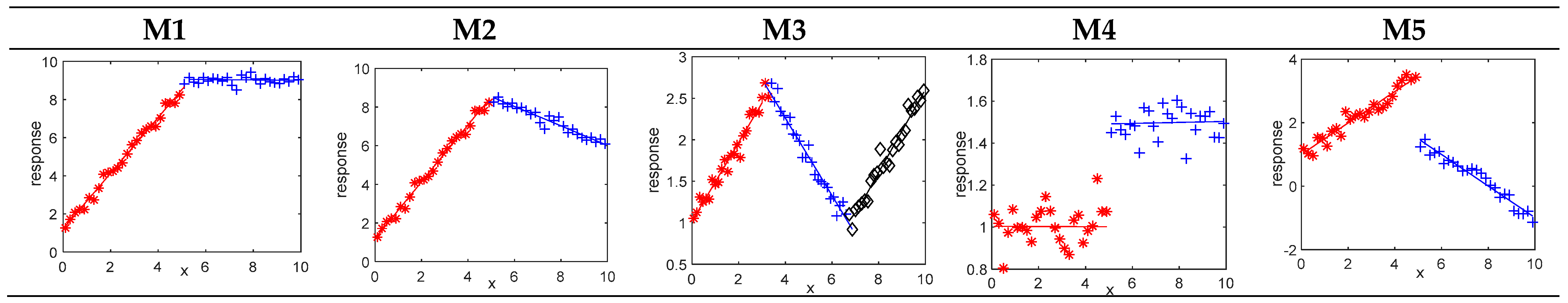
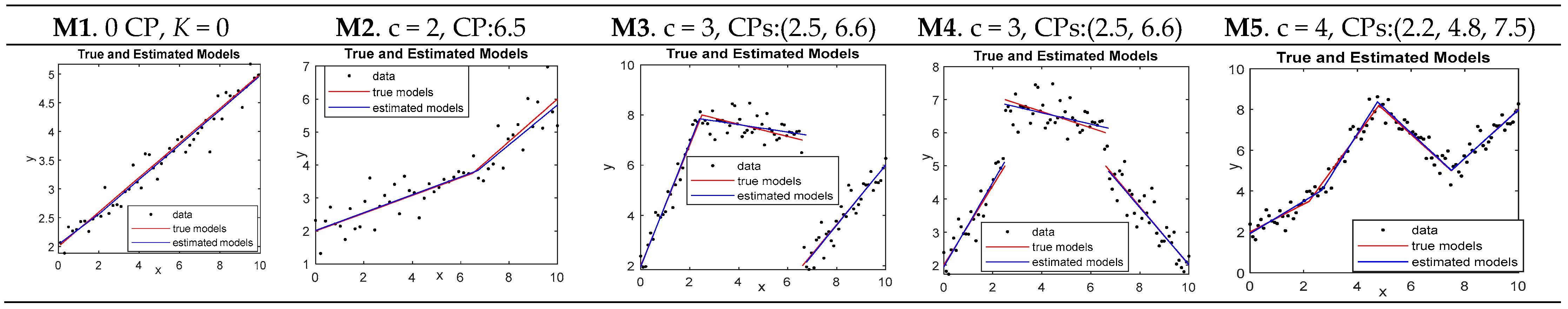
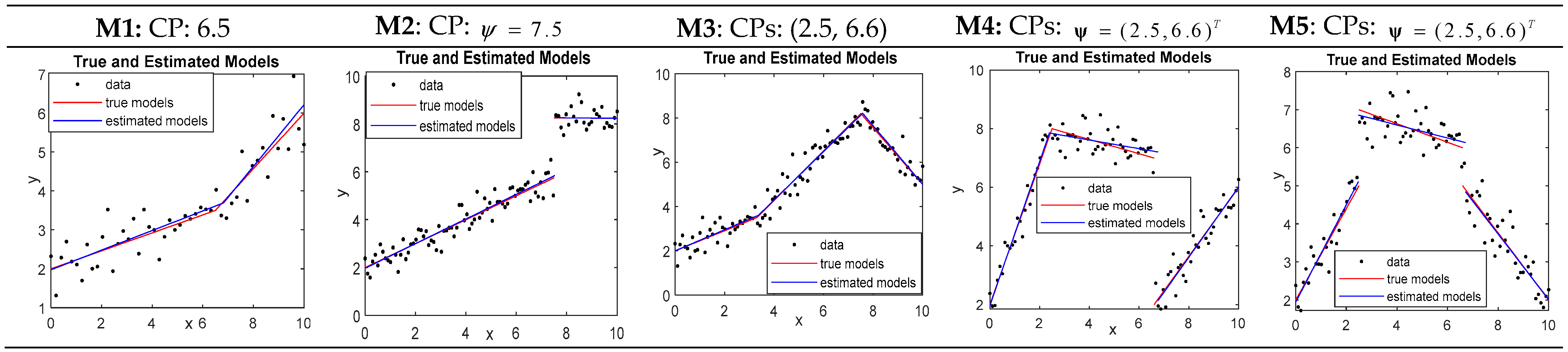
The performance of DSR is first examined based on continuous and discontinuous frames with five different types of models described in

Table 2. Descriptions of four models used in the simulation study.

Model M1: $\psi =6.5$, ${\epsilon }_i\sim N(0,{\sigma }^2)$,$\sigma =0.2$ $y=\left\{\begin{array}{ll}2+0.23077x+{\epsilon }_1,\hfill & \mathrm{if} x\le 6.5,\hfill \\ -1.14286+0.71429x+{\epsilon }_2,\hfill & \mathrm{if} 6.5<x\le 10.\hfill \end{array}\right.$	Model M2: $\psi =6.5$, ${\epsilon }_i\sim N(0,{\sigma }^2)$,$\sigma =0.2$ $y=\left\{\begin{array}{ll}2+0.5x+{\epsilon }_1,\hfill & \mathrm{if} x\le 6.5,\hfill \\ 8.25+{\epsilon }_2,\hfill & \mathrm{if} 6.5<x\le 10.\hfill \end{array}\right.$
Model M3: $\psi ={(3.3,7.5)}^T$, ${\epsilon }_i\sim N(0,{\sigma }^2)$,$\sigma =0.3$ $y=\left\{\begin{array}{ll}2+0.45455x+{\epsilon }_1,\hfill & x\le 3.3,\hfill \\ -0.19286+1.11905x+{\epsilon }_2,\hfill & 3.3<x\le 7.5,\hfill \\ 17.8-1.28x+{\epsilon }_3,\hfill & 7.5<x\le 10.\hfill \end{array}\right.$	Model M4: $\psi ={(2.5,6.6)}^T$; ${\epsilon }_i\sim N(0,{\sigma }^2)$,$\sigma =0.3$ $y=\left\{\begin{array}{ll}2+2.4x+{\epsilon }_1,\hfill & x\le 2.5,\hfill \\ -0.19286+1.11905x+{\epsilon }_2,\hfill & 2.5<x\le 6.6,\hfill \\ 17.8-1.28x+{\epsilon }_3,\hfill & 6.6<x\le 10.\hfill \end{array}\right.$
Model M5: $\psi ={(2.5,6.6)}^T$,${\epsilon }_i\sim N(0,{\sigma }^2)$,$\sigma =0.2$ $y=\left\{\begin{array}{ll}2+1.2x+{\epsilon }_1,\hfill & x\le 2.5,\hfill \\ 7.6098-0.2439x+{\epsilon }_2,\hfill & 2.5<x\le 6.6,\hfill \\ 17.8-1.28x+{\epsilon }_3,\hfill & 6.6<x\le 10.\hfill \end{array}\right.$

. For all models in Table 2, ${\epsilon }_1$,${\epsilon }_2$, and ${\epsilon }_3$ are independent and normally distributed ${\epsilon }_i\sim N(0,{\sigma }^2)$. For illustrative purposes, plots of one simulated sample with the estimated model associated with each individual model in Table 2 are shown in Figure 6.

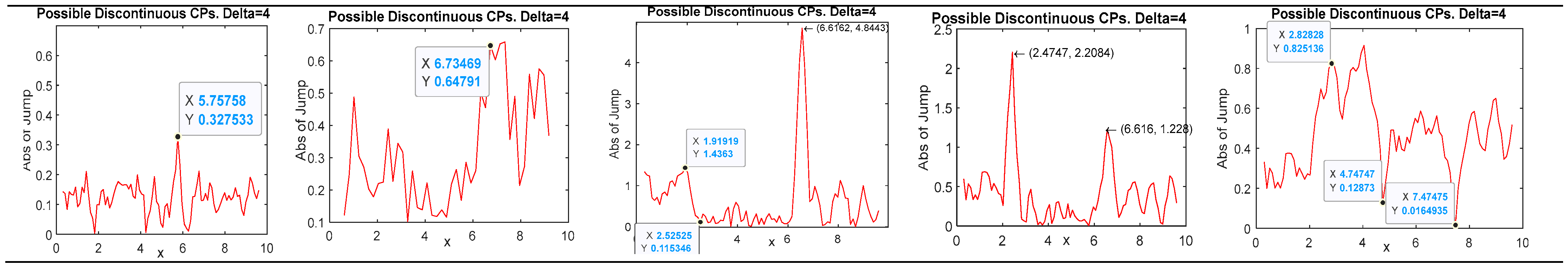
We first evaluate the performance of DSR using Model 4 with simulations carried out under different scenarios: different sample sizes (n), different change-point locations ($\psi$), different standard deviations ($\sigma$). The behavior of change-point estimators is observed on the basis of 1000 replicates through the mean (CPhat) and the standard deviation (stdCP). The IJD was used with the values of $\delta$ (see Section 3.2.1) chosen as 4, 8, and 15 for the sample sizes n = 150, 300, and 600, respectively. The performance of the parameter estimator was accessed by means of 1000 replicates for each model through several measures, defined as follows:

(1)

$\mathrm{CPhat}=\widehat{\psi }=\frac{1}{R}{\displaystyle \sum _{r=1}^R{\widehat{\psi }}_r}$, ${\widehat{\psi }}_r$ is the estimator of ${\psi }_r$, in the rth replication;

(2)

$\mathrm{stdCP}=\mathrm{SD}(\widehat{\psi })={\left[\frac{1}{R-1}{\displaystyle \sum _{r=1}^R{\left({\widehat{\psi }}_r-\widehat{\psi }\right)}^2}\right]}^{1/2}$;

(3)

$\mathrm{SSEC}={\displaystyle \sum _{i,j}\mathrm{MSE}\left({\beta }_{ij}\right)}$, $\mathrm{MSE}\left({\beta }_{ij}\right)=\frac{1}{R}{\displaystyle \sum _{r=1}^R{\left({\widehat{\beta }}_{ij(r)}-{\beta }_{ij}\right)}^2}$, ${\widehat{\beta }}_{ij(r)}$ is the estimator of ${\beta }_{ij(r)}$ in the rth replication;

(4)

RSS and the time (in seconds) consumed by DSR over 1000 replications.

Moreover, the goodness of fit of the fitted model is accessed through a criterion using the concept of statistical tests. Since the considered models are assumed to be normally distributed, the estimator of regression coefficients ${\widehat{\beta }}_i$ follows a multivariate normal distribution $N({\beta }_i,{\sigma }^2{(X_i^T{X}_i)}^{-1})$ (c.f. [46]), where $X_i$ is a matrix in ${\Re }^{n_i\times (p+1)}$, with $X_j^T=(1,x_j^T)=(1,x_{j1},\dots ,x_{jp})$ as its jth row, $j={\psi }_{i-1}+1,\dots ,{\psi }_i$ given ${\psi }_0=0$, ${\psi }_{K+1}=0$, $i=1,\cdots ,(K+1)$ (K is the number of change-points), and $n_i$ is the number of data in the ith segment. Thus, based on the properties of multivariate normal distributions, the random variable $W_i={({\widehat{\beta }}_i-{\beta }_i)}^T{X}_i^T{X}_i({\widehat{\beta }}_i-{\beta }_i)/{\sigma }_i^2$ follows a ${\chi }^2(p+1)$ distribution (c.f. [46]). Utilizing the concept of statistical tests, we think ${\widehat{\beta }}_i$ is acceptable if $W_i\le {\chi }_{0.05}^2(p+1)$. Let $W=\max (W_1,\cdots ,W_{K+1})$. Then, a fitted model can be viewed as acceptable only if $W\le {\chi }_{0.05}^2(p+1)$, which is quite strict.

Table 3. Simulation results of DSR employed to Model M4 in Figure 6 for estimating change-points and regression coefficients (1000 replicates) under different scenarios.

			Chang-Point Estimates				Goodness of Model Fit
$\mathbf{\psi }$	n	$\mathit{\sigma }$	${\widehat{\mathit{\psi }}}_1$	${\widehat{\mathit{\psi }}}_2$	stdCP1	stdCP2	RSS	SSEC	Accept	Time a
(3.3, 6.7)	150	0.3	3.337	6.674	0.115	0.248	21.279	4.828	0.765	1.813
	300	0.3	3.335	6.690	0.043	0.078	33.823	1.365	0.755	2.141
	600	0.8	3.264	6.690	0.385	0.049	416.616	4.380	0.750	3.563
(2, 7)	150	0.3	2.000	7.000	0.000	0.000	12.952	0.221	0.857	3.016
	300	0.3	2.000	7.000	0.000	0.000	26.468	0.109	0.850	3.188
	600	0.8	2.000	7.000	0.009	0.003	378.874	0.422	0.890	4.000

^a The time consumed over 1000 replications is measured in seconds.

reports the simulation results.

As expected, the estimations generally get better when n increases. For instance, under the case $\psi ={(3.3, 6.7)}^T,$ $\sigma =0.3$, the change point estimators with n = 300 are much less varied than those with n = 150, for less stdCP1 (0.043 < 0.115) and stdCP2 (0.078 < 0.248), resulting in a much better fitted model with n = 300, for less SSEC (1.365 < 4.828). Moreover, as $\sigma$ increases to 0.8, the impact of large deviation on the estimators can be alleviated by a larger sample size. For instance, the estimations with n = 600 and $\sigma =0.8$ are almost as good as those with n = 150 and $\sigma =0.3$ in the case of $\psi =(3.3, 6.7)$. The locations of change-points also affect the estimations. Based on many simulations, we found that, if the true change-points were at $\psi =(3.3, 6.7)$, the estimates of change-points and regression coefficients were inferior to those with the true change-points different from $\psi =(3.3, 6.7)$. For example, the estimations with the true change-points at $\psi =(2, 7)$ are better than those with $\psi =(3.3, 6.7)$ in all considered cases (see Table 3). Furthermore, in all cases with $\psi =(2, 7)$, the acceptable proportions of the estimates for regression coefficients are above 85%, which is much higher than those in cases of $\psi =(3.3, 6.7)$ (see Table 3). Note that the case $\psi =(3.3, 6.7)$ means two change-points evenly divide the whole range of independent variable x, $x\in [0,10]$, i.e., the lengths of three sub-segments are equal. It seems reasonable that change-point detection is harder when the length of each sub-segment is the same than when the length of each sub-segment is different. Additionally, the time taken by DSR over 1000 replications with the sample size equal to 600 is very short, and the time increases mildly as n increases (the computational complexity will be discussed later). Therefore, DSR could be applicable to most real data sets effortlessly. Specifically, Seber [1] commented that piecewise regression models are intended for circumstances where the number of regimes is small and there are fairly sharp changes between sub-segments. Muggeo [4] also mentioned that a few change-points might be enough for dealing with practical situations, and the significance of change-points may become disputable as the number of change-points gets large. Thus, DSR could be a very practical technique for solving change-point regression problems.

Next, we compare the proposed DSR with the following four methods: the segmented method (SEG) [4], the EM-BP algorithm [12], the FCP algorithm [47], and the FCM-BP method (FCM) [12]. The estimations for change-points and regression coefficients are observed on the basis of 1000 and 200 replicates with the sample of size equal to 50 and 100 for models of one and multiple change-points, respectively. Note that the sample sizes utilized in the comparisons are small because the existing methods are very time-consuming due to their high computational cost. The measures used for making comparisons are the same as those used earlier for evaluating DSR.

Table 4. Comparisons of DSR with existing methods using 1 CP Models (M1 and M2) in Figure 6.

(a) M1. n = 50	$\mathit{\psi } = 6.5$	stdCP	RSS	SSEC	Accept	Time a
DSR	6.480	0.582	2.659	0.812	0.759	0.594
SEG	6.341	0.315	1.850	0.208	0.837	0.297
EM-BP	6.597	0.524	1.870	0.395	0.803	1.938
FCP	6.474	0.579	3.259	1.803	0.815	1.125
FCM	6.488	0.590	1.787	0.274	0.821	0.828
(b) M2, n = 50	$\mathit{\psi } = 7.5$	stdCP	RSS	SSEC	Accept	Time
DSR	7.449	0.000	1.839	0.417	0.900	1.250
SEG	5.606	0.244	12.923	83.094	0.000	0.828
EM-BP	7.347	0.000	1.839	0.417	0.900	0.563
FCP	7.347	0.000	1.842	0.437	0.898	0.484
FCM	7.345	0.065	1.848	0.486	0.899	0.484

^a The time consumed over 1000 replications is measured in seconds.

and

Table 5. Comparisons of DSR with existing methods using 2 CP Models (M3-M5) in Figure 6.

M3, n = 100	${\mathit{\psi }}_1$ = 3.3	stdCP1	${\mathit{\psi }}_2$ = 7.5	stdCP2	RSS	SSEC	Accept	Time a
DSR	3.299	0.069	7.498	0.022	0.944	0.068	0.850	0.250
SEG	3.299	0.069	7.498	0.022	0.944	0.068	0.850	0.250
EM-BP	3.272	0.245	7.500	0.000	0.917	0.053	0.920	765.750
FCP	3.301	0.217	7.500	0.000	0.924	0.059	0.730	17.578
FCM	3.304	0.223	7.500	0.000	0.915	0.048	0.840	16.047
M4, n = 100	${\mathit{\psi }}_1$ = 2.5	stdCP1	${\mathit{\psi }}_2$ = 6.6	stdCP2	RSS	SSEC	Accept	Time
DSR	2.500	0.067	6.611	0.039	10.656	0.244	0.81	0.516
SEG	2.502	0.064	6.115	0.053	11.935	2.212	0.01	0.188
EM-BP	2.480	0.231	6.600	0.014	8.187	0.267	0.79	303.938
FCP	2.508	0.183	6.589	0.092	8.245	0.348	0.75	20.188
FCM	2.499	0.178	6.589	0.091	8.156	0.258	0.83	19.625
M5, n = 100	${\mathit{\psi }}_1$ = 2.5	std1	${\mathit{\psi }}_2$ = 6.6	std2	RSS	SSEC	Accept	Time
DSR	2.510	0.083	6.485	0.305	4.134	0.362	0.725	0.453
SEG	3.141	0.053	5.791	0.123	13.265	2.509	0	0.250
EM-BP	2.495	0.036	3.741	0.475	11.381	5.836	0.04	206.234
FCP	2.500	0.000	6.596	0.045	3.891	0.348	0.47	24.109
FCM	2.500	0.000	6.600	0.000	3.700	0.110	0.84	13.938

^a The time consumed over 1000 replications is measured in seconds.

report the estimations for the five models given in Table 2 by using the five methods, respectively.

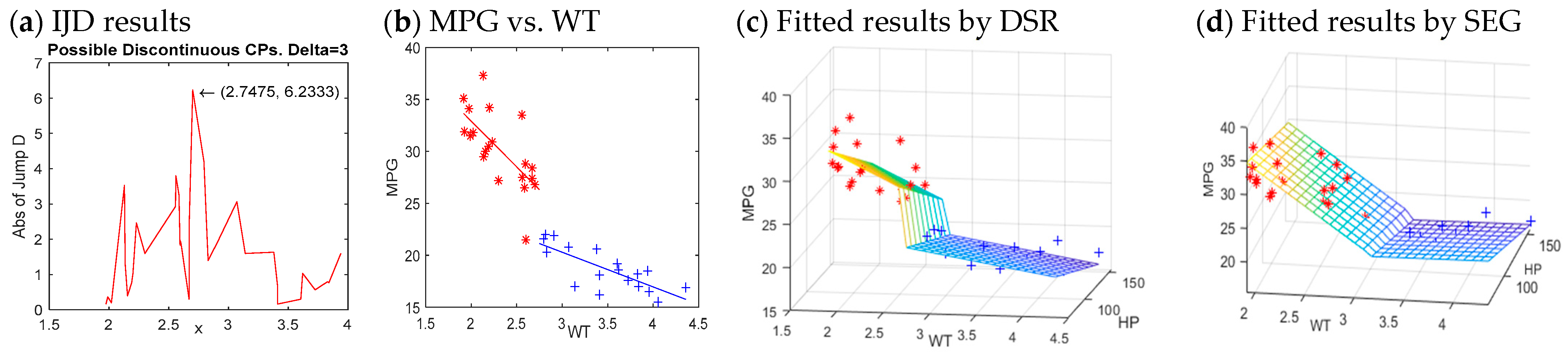
Table 4 shows that SEG performs best in the estimations for model M1 because SEG produced a change-point estimator with very small biases and variations (note that the stdCP obtained by SEG equal to 0.315 is the least small among the five methods). Furthermore, SEG results in the best fitted model with the least SSEC (0.208) and the highest acceptance rate (0.837). However, SEG is totally unworkable for the discontinuous model M2. On the other hand, the other four methods also perform well in all cases reported in Table 4. They are competitive in the estimations for models M1 and M2 regarding the precision and variation of the change-point estimators and the adequacy of the estimated model.

For the estimations of multiple change-point models M3-M5 shown in Table 5, DSR generally outperforms the other four methods for producing highly accurate estimates of change-points and regression coefficients in a very short time. In particular, DSR is much more economical in terms of time-consumption than the EM-BP, FCP, and FCM. In particular, the time consumed by EM-BP is extremely high. Even worse, EM-BP could not produce adequate estimates for model M5 due to a very large bias with the estimate of ${\psi }_2$ (bias = 6.6 − 3.741 = 2.859) and the poor fit of the estimated model with a large SSEC (5.836) and a very low acceptance rate (0.04). Although the estimations made by FCP and FCM for M3-M5 are satisfactory, they are also much more computationally expensive than DSR. Notice that the time taken by FCP and FCM looks tolerable because of the small sample size, n, and the small number of change-points, K. In fact, their computational complexity increases drastically with n and k, and the computational time would increase drastically even if n or K increased slightly. This evidence can be understood through the computational complexity analysis below.

We noted from the above comparisons that the superiority of DSR over EM-BP, FCP, and FCM is particularly significant in view of time consumption. This fact can be attributed to the incorporation of IJD with DSR and the much less complexity of DSR. IJD helps DSR converge faster by producing suitable initial values to be used (see the illustrations of IJD in Section 3.2). But the computational complexity may account for the preference of DSR mostly. The computational complexity of DSR is $O\left(n(K+1)di\right),$ where n is the data size, K is the number of regimes, d is the data dimension, and i is the number of iterations. For EM-BP, FCP, and FCM, the computations for estimated parameters must be performed for each possible collection of change-points which include $C_K^n$ combinations. Thus, the computational complexity of EM-BP, FCP, and FCM is $O\left(n^K(K+1)di\right)$. That may be the reason why the time consumed by DSR is much less than that of the other three methods as the number of change-points increases.

Table 6. Comparisons between DSR and EM-BP in the time (in seconds) consumed over 1000 replicates or fewer.

Model, K, i	M1, K = 1, 1000	M2, K = 1, 1000	M3, K = 2, 200	M4, K = 2, 200	M5, K = 2, 200
DSR $O\left(n(K+1)di\right)$ a	0.594	1.250	0.250	0.516	0.453
EM-BP $O\left(n^K(K+1)di\right)$	1.938	0.563	765.750	303.938	206.234
FCP $O\left(n^K(K+1)di\right)$	1.125	0.484	17.578	20.188	24.109
FCM $O\left(n^K(K+1)di\right)$	0.828	0.484	16.047	19.625	13.938

^a n: the sample size, K: the number of change-points, d: the data dimension, i: the number of iterations.

summaries the time consumed by DSR, EM-BP, FCP, and FCM in the cases used for comparisons previously. Note the simulation results shown in Table 4 and Table 5 are based on 1000 and 200 replications for one and multiple change-points in the models, respectively. The results in Table 6 indicate that the time taken by DSR increases slowly with the number of change-points, K. But the time taken by the other three methods increases sharply as K increases, especially for EM-BP. Notice that the time consumed by DSR in case M2 is much higher due to the detection of jumps.

To sum up, the comparison results obtained with the models in Table 2 reveal that DSR can work well in all cases of continuous and discontinuous models. More importantly, DSR produces better estimates for change-points and regression coefficients in virtue of smaller biases and variations of change-point estimators, as well as the small mean squared errors of estimated regression coefficients in almost all cases of continuous and discontinuous models. Moreover, DSR is much more economic in terms of the time consumed than EM-BP, FCP, and FCM, especially in cases involving multiple change-points. By contrast, SEG performs well for continuous models but is totally unworkable for discontinuous models. Simulation results show that the time consumed by DSR over 1000 replications increases slowly with K. This fact indicates that the computational effort of DSR increases mildly with the complexity of the model. As remarked by Muggeo [4] and Seber [1], piecewise regression models with a few change-points are sufficient for handling many practical situations because the meaning of change-points may become questionable as the number of regimes increases. Thus, the proposed DSR is feasible for most practical problems.

4.2. Real Applications

We demonstrate the practicability of the proposed DSR through five real examples from different areas.

Example 1.

We employed the proposed DSR to a data set previously analyzed by [8,12,47]. The data set includes the measurements of three variables, miles per gallon (MPG), weight (WT), and horsepower (HP) on 38 automobiles of different models made in 1978–1979. The three papers concluded that the following segmented representation given by (22) is the best model based on the modified Schwarz’ Criterion (c.f. [8]) and the mean of the residual sum of squares (MRS) defined in (23) respectively.

$$\begin{array}{cc}E(MPG)={\beta }_{10}+{\beta }_{11}WT+{\beta }_{12}HP,& \mathrm{if} WT\le \tau , \\ E(MPG)={\beta }_{20}+{\beta }_{21}WT+{\beta }_{22}HP,& \mathrm{if} WT>\tau .\end{array}$$

(22)

The mean of the residual sum of squares (MRS) is

$$\mathrm{MRS}=RSS(K)/[n-(K+1)(p+1)]={\displaystyle \sum {(y_i-{\widehat{y}}_i)}^2}/[n-(K+1)(p+1)],$$

(23)

where K is the number of change-points. They also concluded that the dependence of MPG on WT and HP shows an abrupt change after WT becomes larger than 2.7 (in 1000 lbs). The graphical display of data in Figure 7b,c also discloses a jump in the relationship between MPG and WT when$WT\in (2.5, 3)$. As suggested by these three previous papers, we applied DSR to the car data using model (22). A possible discontinuous jump at (2.7475, 6.2333) is detected (see Figure 7a) by using IJD and DSR and the resulted model is

$$E(MPG)=\left\{\begin{array}{cc}48.82-5.23WT-0.08HP,& WT\le 2.7475,\\ 30.76-1.84WT-0.05HP,& WT>2.7475.\end{array}\right..$$

The model produced by DSR is very close to those obtained by [8,12,47]. Moreover, we also utilized Muggeo’s SEG to the car data with model (22), resulting in a fitted model graphically shown in Figure 7d, with a change-point at WT = 3.1375. Apparently, the estimated change-point by SEG (see Figure 7b,c) is irrational. This further illustrates the failure of SEG in detecting discontinuous jumps.

Example 2.

The climate trend research is important for understanding the development of global warming, which has been a world-wide issue and received great attention. Regression analysis has been adopted by several researchers [48,49] to analyze the changes in climate tendency. Many studies pointed out that the most remarkable change in the time series of global temperature occurred during the 1970s. We implemented DSR to the global temperature data, HadCRUT3, collected by the Met Office Hadley Center, also studied by [12,49]. The irregularities of the global temperature were re-computed, with the mean of temperatures over the period 1961–1990 regarded as the baseline. Figure 8 exhibits the estimated results obtained by DSR. Figure 8a indicates that there is no significant jump in the temperature series, but relatively large deviations appear at several places; for example, around the years 1901, 1945, and 1978, connected change-points may exist. Referring to the comments made by [4,6], piecewise models are intended for situations where the number of segments is small. Muggeo [4] suggested that a few change-points (e.g., one to three) for a sample of moderate size may be sufficient for dealing with several practical circumstances, since the implication of change-points might become questionable as the number of change-points increases. Thus, we fitted the data using piecewise regression models with the number of change-points K = 1, 2, and 3, respectively. According to the illustrations on the use of IJD in Section 3.2.2, the plots in Figure 8a indicate that no discontinuous jump was detected, but D_i shows three relatively large variations around the years 1901, 1945, and 1978, suggesting the existence of three connected change-points.

Table 7. The estimates of HadCRUT3 data derived via DSR with K = 1, 2, and 3, respectively.

K, CP	K = 1, CP: 1971	K = 2, CPs: 1905, 1975	K = 3
coefficients	${\widehat{\beta }}_{11}=0.00356$, ${\widehat{\beta }}_{21}=0.01656$	${\widehat{\beta }}_{11}=-0.00444,$ ${\widehat{\beta }}_{21}=0.00536,$ ${\widehat{\beta }}_{31}=0.01535,$	x
RSS	1.683	1.219	1.228
MRS	0.013	0.009	0.010

$\mathrm{MRS}=RSS(K)/[n-(K+1)(p+1)]={\displaystyle \sum {(y_i-{\widehat{y}}_i)}^2}/[n-(K+1)(p+1)]$, where K is the number of change-points.

reports the estimations for models with different K values. With K = 1, DSR produced a noteworthy change in 1971, which is in accordance with the finding of previous research [49]. However, when comparing the MRS resulted from models with different K values, the three-segment model in Figure 8c is preferable because it presents the smallest MRS among the three models considered in Table 7. Furthermore, the development of temperature changes can be seen more clearly and completely through the three-segment model. The fitted lines in Figure 8c and the estimations in Table 7 indicate there is no significant relation between global temperature and time before 1905. After 1905, the temperature started increasing with time gradually and the increasing speed became much faster after 1975. These discoveries illustrate the much faster rate of global warming effect in recent years.

Example 3.

We employ DSR to the data set including measurements of the annual volume (in 10⁸ m³) of discharge from the Nile River at Aswan, from year 1871 to 1970. The researchers [50,51] wanted to know whether abrupt changes in the mean of the annual discharge occur at some time points during this period. The plot of the data shown in Figure 9b reveals that the mean discharges decreased with time from the beginning (year 1871), followed a markedly large decrease around point 40 (year 1940), and then remains constant after the time of extremely low discharge. Figure 9a shows two possible jumps at time points 40.5 and 45.5. Thus, we fitted the data with models of two and three segments, respectively. Figure 9c indicates that the annual mean discharge decreased with time significantly (${\widehat{\beta }}_{11}=-6.687$) before point 40, i.e., year 1910. Note that the jump detected at 40.5 is because of the occurrence of an exceptionally low discharge around point 40. As commented by Cobb [50], the abnormally low change is real and can be found in the records of tropical weather stations. Both models (b) and (c) in Figure 9 demonstrate that the mean annual discharge remains constant around 861 (in 10⁸ m³) after point 45 (year 1915). As remarked by Zeileis et al. [51], the unchanged mean discharge from the Nile River after 1915 may be partly attributed to the operation of the Aswan dam, starting from 1902.

Example 4.

Change-point detection is important in the context of quality control. This example considers a dataset from manufacturing. The data analyzed by Lombard [52], Lu and Chang [11,13] contain 100 radii of consecutive circular indentations made by a milling machine, which were obtained for comparing the effects of two service routines on the productions of the machine. The estimated results by DSR are shown in Figure 10. IJD produced two potential jumps at time point 52.5 and 82.5 respectively. Therefore, we fitted the data with models including two and three pieces, respectively. Both models in Figure 10b,c present a precipitous change at point 82, after which the radii significantly increase with time for the estimated slope$\widehat{\beta }=0.0112$, which is significantly different from 0. Moreover, the estimated slope of the second line inFigure 10c is very small (${\widehat{\beta }}_{21}=-0.0003$), and the mean of the residual sum of squared errors for the two models is the same, i.e., MRS(2) equals MRS((1). Thus, in view of the parsimony in model selections, the two-segment model in Figure 10b is an adequate model to the milling machine data. The resulted model by DSR indicates a sharp jump in the radii data at time point 82. After the change-point at 82, the radii data significantly increase with time.

Example 5.

In this example, we employ DSR to the well-log data (c.f. [53]), which include 4050 measurements of nuclear magnetic response obtained when digging a well. Sharp shifts in the mean of the process measurements often occur at the transitions of rock strata. Thus, locating change-points is crucial for oil drilling (c.f. [13,53]). We applied DSR to a subset of indexed measurements from 2000 to 2650. DSR resulted in five potential discontinuous change-points at 2046.5, 2409.5, 2469.5, 2531.5, and 2591.5, respectively, which are close to the apparent five jumps shown in Figure 11b. The final estimated model with five abrupt jumps at 2046, 2409, 2469, 2531, 2591 is reasonable. Thus, the proposed DSR identified the five jump points properly.

5. Conclusions and Discussion

In this paper, we have introduced an advanced piecewise regression model for dealing with regression relationships with abrupt changes. The main advantage of the proposed piecewise model is its availability for problems with discontinuous and/or continuous change-points. Fong et al. [54] emphasized that it is really challenging to recognize whether any jump occurs somewhere, making it difficult to choose proper methods to analyze data. This indicates the difficulty of jump point detection. It may be the reason why many existing methods are restricted to continuous models, e.g., [4,7,28,30,32]. However, continuity cannot be simply assumed in a real problem, unless it is known theoretically. In practice, continuity may be highly probable in medical or biological problems, but it may not be appropriate for problems in economics, finance, or geological prospecting (c.f. [36]). Thus, the flexibility of the proposed piecewise model in dealing with both continuous and discontinuous change-point locations is very useful in practice.

A new algorithm, called DSR, has been proposed for estimating piecewise regression models. A linear Taylor expansion has been adopted to circumvent the non-smoothness of the likelihood function. Accordingly, the estimation for piecewise models is simplified to the iterative fitting of linear regression models. The estimates of change-points and regression parameters can be obtained. The new approach has the advantages of being simple, fast, and highly efficient, regardless of whether the piecewise regression model is continuous or not. Furthermore, the proposed model is feasible for fitting generalized linear models, whereas the IJD method is less sensitive in the cases of generalized linear models. The regression errors can follow other distributions such as t, Laplace, or a mixture of normal distributions. The least squared error estimations can be replaced by the least absolute deviation criterion for obtaining more robust estimators. With the utilization of first-order Taylor approximations, the DSR algorithm is like a Gauss-Newton-based method. Thus, DSR is convergent provided that suitable initial values are used (c.f. [1], pp. 25–26). Muggeo [4] also noted that the segmented approach using linear approximations can be shown to be exact, ensuring so that it will always converge in a deterministic model provided that the change-point exists. Simulation results have demonstrated that for Gaussian data with moderate variance, DSR, with appropriate starting points, always attains the correct solutions with negligible biases. Therefore, if the DSR algorithm fails in some cases, it may be due to improper initial values or a particular configuration of data (for instance, too few data points contained in a regime to estimate parameters, or when the relationship is unstable).

Since the performance of DSR depends on initialization, the IJD method has been created for detecting possible jump points. The IJD method is helpful for accelerating the convergence of DSR because of the proper starting values chosen. The IJD method may be also informative in finding potential connected change-points. The incorporation of IJD with the idea of [41,45] is a practical tool for determining the number of change-points.

Several examples with numerical datasets demonstrated the effectiveness and superiority of the proposed DSR. The preference of DSR was particularly significant in the aspect of computational efficiency, especially in cases of multiple change-points. The applications to several real datasets from diverse areas indicate the wide applicability of DSR.

Multicollinearity is an issue often considered in regression analysis. Specifically, for fitting piecewise regression models, there is a chance to have multicollinearity on the design matrix of $X$ variables, which leads to the problem that the matrix $X{X}^{\prime }$ in the normal equation is singular or close to singular. There are three causes of the multicollinearity problem in piecewise regressions:

• A poor dataset;
• Overfitting due to the number of change-points used for estimations larger than the true one;
• Too few data points contained in one (or more than one) regime to estimate regression coefficients during the iteration process.

Possible strategies for handling multicollinearity problems include:

• Re-assign new initial values (change points), especially for those problems resulting from cause 3;
• Apply the Ridge regression estimators (c.f. [55]).

An important merit of the Ridge regression strategy is that it always works for a singular or close to singular matrix only if a proper nonnegative biasing constant c is chosen. Since the biasing constant c reflects the amount of bias in the estimations, we apply Ridge regressions with a very small c (say, less than 1.0 × 10⁻¹⁰) for cases having a singular matrix, with c = 0 for cases without having a singular matrix. It is possible that a singular matrix occurs in one fitting iteration, and it turns out to be the occurrence of a non-singular matric in the following fitting iteration after the application of the Ridge method.

For our future work, we consider relaxing the linearity assumption. For some real data, linear regression lines cannot work well, but higher orders of polynomial may perform better. For example, the results in Figure 12 show that simple linear regression lines cannot produce adequate estimates for change-points and regression parameters, but third-degree models fit the data well and provide reasonable estimates for change-points. Moreover, the variance is assumed to be constant over all subdivisions, but the heterogeneity of variances occurs often in change-point problems. We consider relaxing these assumptions in the future work. The weighted least squares estimations may be helpful for handling the problem of heterogeneity. As to the approximation by higher order polynomials, it is much more complicated than first-order approximation. Just as stated in [56], higher order polynomials are much more difficult to deal with. More effort and deeper thinking are needed to find a feasible approach.

Moreover, the problems of outliers and missing data are often encountered in regression analysis. Possible feasible methods for alleviating the influence of outliers include using the absolute least deviation method instead of the least squares estimations or assuming model errors having t or Laplace distributions to increase the resistance of estimators against outliers. As to the problem of missing data, several techniques of dealing with missing data may be useful, but they need further research. These are important and difficult problems in regression analysis. Further studies on these issues are required in the future.

References

1. Seber, G.A.F.; Wild, C.J. Nonlinear Regression; Wiley: New York, NY, USA, 2003. [Google Scholar]
2. Perperoglou, A.; Sauerbrei, W.; Abrahamowicz, M.; Schmid, M. A review of spline function procedures in R. BMC Med. Res. Methodol. 2019, 19, 1–16. [Google Scholar] [CrossRef] [PubMed]
3. Ren, J.; Tapert, S.; Fan, C.C.; Thompson, W.K. A semi-parametric Bayesian model for semi-continuous longitudinal data. Stat. Med. 2022, 41, 2354–2374. [Google Scholar] [CrossRef] [PubMed]
4. Muggeo, V.M.R. Estimating regression models with unknown breakpoints. Stat. Med. 2003, 22, 3055–3071. [Google Scholar] [CrossRef] [PubMed]
5. Fearnhead, P.; Rigaill, G. Changepoint Detection in the Presence of Outliers. J. Am. Stat. Assoc. 2019, 114, 169–183. [Google Scholar] [CrossRef]
6. Ulm, K. A statistical methods for assessing a threshold in epidemiological studies. Stat. Med. 1991, 10, 341–349. [Google Scholar] [CrossRef] [PubMed]
7. Zhang, F.; Li, Q. Robust bent line regression. J. Stat. Plan. Inference 2017, 185, 41–55. [Google Scholar] [CrossRef] [PubMed]
8. Liu, J.; Wu, S.; Zidek, J.V. On segmented multivariate regression. Stat. Sin. 1997, 7, 497–525. [Google Scholar]
9. MacNeill, I.B.; Mao, Y. Change-point analysis for mortality and morbidity rate. In Applied Change Point Problems in Statistics; Sinha, B., Rukhin, A., Ahsanullah, M., Eds.; Nova Science: Hauppauge, NY, USA, 1995; pp. 37–55. [Google Scholar]
10. Ruanaidh, J.J.K.Ó.; Fitzgerald, W.J. Numerical Bayesion Methods Applied to Signal Processing; Springer: New York, NY, USA, 1996. [Google Scholar]
11. Lu, K.P.; Chang, S.T. Change-point detection for shifts in control charts using fuzzy shift change-point algorithms. Comput. Ind. Eng. 2016, 93, 12–27. [Google Scholar] [CrossRef]
12. Lu, K.P.; Chang, S.T. A fuzzy classification approach to piecewise regression models. Appl. Soft Comput. 2018, 69, 671–688. [Google Scholar] [CrossRef]
13. Lu, K.P.; Chang, S.T. Fuzzy maximum likelihood change-point algorithms for identifying the time of shifts in process data. Neural Comput. Appl. 2019, 31, 2431–2446. [Google Scholar] [CrossRef]
14. Bardwell, L.; Fearnhead, P. Bayesian detection of abnormal segments in multiple time series. Bayesian Anal. 2017, 12, 193–218. [Google Scholar] [CrossRef]
15. Melnyk, I.; Banerjee, A. A spectral algorithm for inference in hidden semi-Markov models. J. Mach. Learn. Res. 2017, 18, 1–39. [Google Scholar]
16. Haynes, K.; Fearnhead, P.; Eckley, I.A. A computationally efficient nonparametric approach for changepoint detection. Stat. Comput. 2017, 27, 1293–1305. [Google Scholar] [CrossRef] [PubMed]
17. Garreau, D.; Arlot, S. Consistent change-point detection with kernels. arXiv 2016, arXiv:1612.04740. [Google Scholar] [CrossRef]
18. Frick, K.; Munk, A.; Sieling, H. Multiscale change point inference. J. R. Stat. Soc. Ser. B Stat. Methodol. 2014, 76, 495–580. [Google Scholar] [CrossRef]
19. Pein, F.; Sieling, H.; Munk, A. Heterogeneuous change point inference. J. R. Stat. Soc. Ser. B Stat. Methodol 2017, 79, 1207–1227. [Google Scholar] [CrossRef]
20. Fryzlewicz, P. Wild binary segmentation for multiple change-point detection. Ann. Stat. 2014, 42, 2243–2281. [Google Scholar] [CrossRef]
21. Korkas, K.; Fryzlewicz, P. Multiple change-point detection for non-stationary time series using wild binary segmentation. Stat. Sin. 2017, 27, 287–311. [Google Scholar] [CrossRef]
22. Haynes, K.; Eckley, I.A.; Fearnhead, P. Computationally Efficient Changepoint Detection for a Range of Penalties. J. Comput. Graph. Stat. 2017, 26, 134–143. [Google Scholar] [CrossRef]
23. Elhanashi, A.; Gasmi, K.; Begni, A.; Dini, P.; Zheng, Q.; Saponara, S. Machine Learning Techniques for Anomaly-Based Detection System on CSE-CIC-IDS2018 Dataset. In Applications in Electronics Pervading Industry, Environment and Society. ApplePies 2022. Lecture Notes in Electrical Engineering; Springer: Cham, Switzerland, 2023; p. 1036. [Google Scholar] [CrossRef]
24. Lu, K.P.; Chang, S.T. Robust algorithms for multiphase regression models. Appl. Math. Model. 2020, 77, 1643–1661. [Google Scholar] [CrossRef]
25. Lu, K.P.; Chang, S.T. Robust Algorithms for Change-Point Regressions Using the t-Distribution. Mathematics 2021, 9, 2394. [Google Scholar] [CrossRef]
26. Lu, K.P.; Chang, S.T. Robust Switching Regressions Using the Laplace Distribution. Mathematics 2022, 10, 4722. [Google Scholar] [CrossRef]
27. Truong, C.; Oudre, L.; Vayatis, N. Selective review of offline change point detection methods. Signal Process. 2010, 167, 107299. [Google Scholar] [CrossRef]
28. Muggeo, V.M.R. Segmented: An R package to fit regression models with broken-line relationships. News. R Proj. 2008, 8, 20–25. [Google Scholar]
29. Muggeo, V.M.R.; Attanasio, M.; Porcu, M. A segmented regression model for event history data: An Application to fertality Patterns in Italy. J. Appl. Stat. 2009, 36, 973–988. [Google Scholar] [CrossRef]
30. Muggeo, V.M.R.; Adelfio, G. Efficient change point detection for genomic sequences of continuous measurements. Bioinformatics 2011, 27, 161–166. [Google Scholar] [CrossRef] [PubMed]
31. Muggeo, V.M.R.; Atkins, D.C.; Gallop, R.J.; Dimidjian, S. Segmented mixed models with random changepoints: A maximum likelihood approach with application to treatment for depression study. Stat. Model. 2014, 14, 293–313. [Google Scholar] [CrossRef]
32. Shi, S.; Li, Y.; Wan, C. Robust continuous piecewise linear regression model with multiple change points. J. Supercomput. 2018, 76, 1–23. [Google Scholar] [CrossRef]
33. Muggeo, V.M.R.; Sottile, G.; Porcu, M. Modelling COVID-19 outbreak: Segmented regression to assess lockdown effectiveness. Tech. Rep. 2020, 10, 16. [Google Scholar] [CrossRef]
34. Küchenhoff, H.; Günther, F.; Höhle, M.; Bender, A. Analysis of the early Covid-19 epidemic curve in Germany by regression models with change points. Epidemiol. Infect. 2020, 149, e68. [Google Scholar] [CrossRef]
35. Shaukat, M.H.; Alotaibi, N.; Hussain, I.; Shrahili, M. The Analysis of the Incidence Rate of the COVID-19 Pandemic Based on Segmented Regression for Kuwait and Saudi Arabia. Hindawi Math. Problems Eng. 2021, 2021, 2644506. [Google Scholar] [CrossRef]
36. Chen, C.W.S.; Chan, J.S.; Gerlach, K.R.; Hsieh, W.Y.L. A comparison of estimators for regression models with change points. Stat. Comput. 2011, 21, 395–414. [Google Scholar] [CrossRef]
37. Alipour, P.; Bastani, A.F. Value-at-Risk-Based Portfolio Insurance: Performance Evaluation and Benchmarking Against CPPI in a Markov-Modulated Regime-Switching Market. arXiv 2023, arXiv:2305.12539. [Google Scholar]
38. Yang, H.Q.; Xing, S.G.; Wang, Q.; Li, Z. Model test on the entrainment phenomenon and energy conversion mechanism of flow-like landslides. Eng. Geol. 2018, 239, 119–125. [Google Scholar] [CrossRef]
39. Yang, H.; Wang, Z.; Song, K. A new hybrid grey wolf optimizer-feature weighted-multiple kernel-support vector regression technique to predict TBM performance. Eng. Comput. 2020, 38, 2469–2485. [Google Scholar] [CrossRef]
40. Yang, M.S.; Nataliani, Y. Robust-learning fuzzy c-means clustering algorithm with unknown number of clusters. Pattern Recognit. 2017, 71, 45–59. [Google Scholar] [CrossRef]
41. Hawkins, D.M. Fitting multiple change-point models to data. Comput. Stat. Data Anal. 2001, 37, 323–341. [Google Scholar] [CrossRef]
42. Beckman, R.J.; Cook, R.D. Testing for two-phase regressions. Technometrics 1979, 21, 65–69. [Google Scholar] [CrossRef]
43. Yao, Y.C. Estimating the number of change-points via Schwarz’ criterion. Statist. Probab. Lett. 1988, 6, 181–189. [Google Scholar] [CrossRef]
44. Ciuperca, G. A general criterion to determine the number of change-points. Statist. Probab. Lett. 2011, 81, 1267–1275. [Google Scholar] [CrossRef]
45. Venter, J.H.; Steel, S.J. Finding multiple abrupt change points. Comput. Stat. Data Anal. 1996, 22, 481–504. [Google Scholar] [CrossRef]
46. Hogg, R.V.; McKean, J.W.; Craig, A.T. Introduction to Mathematical Statistics, 7th ed.; Pearson: London, UK, 2013. [Google Scholar]
47. Chang, S.T.; Lu, K.P.; Yang, M.S. Fuzzy Change-point algorithms for regression models. IEEE Trans. Fuzzy Syst. 2015, 23, 2343–2357. [Google Scholar] [CrossRef]
48. Menne, J.M. Abrupt global temperature change and the instrumental record. In Proceedings of the 18th Conference on Climate Variability and Change, Atlanta, GA, USA, 29 January–2 February 2005; p. 4. [Google Scholar]
49. Werner, R.; Valev, D.; Danov, D.; Guineva, V. Study of structural break points in global and hemispheric temperature series by piecewise regression. Adv. Space Res. 2015, 56, 2323–2334. [Google Scholar] [CrossRef]
50. Cobb, G.W. The Problem of the Nile: Conditional solution to a changepoint problem. Biometrika 1978, 65, 243–251. [Google Scholar] [CrossRef]
51. Zeileis, A.; Kleiber, C.; Krämer, W. Testing and dating of structural changes in practice. Comput. Stat. Data Anal. 2003, 44, 109–123. [Google Scholar] [CrossRef]
52. Lombard, F. Rank tests for changepoint problems. Biometrika 1987, 74, 15–624. [Google Scholar] [CrossRef]
53. Neubauer, J.; Vesely, V. Detection of multiple changes in mean by sparse parameter estimation. Nonlinear Anal. Model. Control 2013, 18, 177–190. [Google Scholar] [CrossRef]
54. Fong, Y.; Huang, Y.; Gilbert, P.B.; Permar, S.R. chngpt: Threshold regression model estimation and inference. BMC Bioinform. 2017, 18, 454. [Google Scholar] [CrossRef]
55. Kutner, M.H.; Nachtseim, C.J.; Neter, J.; Li, W. Applied Linear Statistical Models; McGraw-Hill Irwin: New York, NY, USA, 2005. [Google Scholar]
56. Box, G.E.P.; Tidwell, P.W. Transformation of the Independent Variables. Technometrics 1962, 4, 531–550. [Google Scholar] [CrossRef]
Figure 1. Some possible continuous or discontinuous broken-line regressions with one or two break- points.
Mathematics 11 04959 g001
Figure 2. Scatter plots of well-log data and the car data with MPG vs. WT.
Mathematics 11 04959 g002
Figure 3. DSR depends on initialization using continuous and discontinuous models, respectively, and IJD works for providing suitable initials.
Mathematics 11 04959 g003
Figure 4. Graphic presentation of the IJD method for detecting possible jump points at the point indicated by an arrow with the corresponding coordinates.
Mathematics 11 04959 g004
Figure 5. Models used for illustrating the determination of the number of segments by the suggested indices.
Mathematics 11 04959 g005aMathematics 11 04959 g005b
Figure 6. Plots of a simulated sample associated with each individual model used for comparisons.
Mathematics 11 04959 g006
Figure 7. The fitted results of the car data produced by DSR.
Mathematics 11 04959 g007
Figure 8. The fitted results of the global temperature data (HadCRUT3) by DSR.
Mathematics 11 04959 g008
Figure 9. The fitted results of the Nile River data by DSR.
Mathematics 11 04959 g009
Figure 10. The fitted results of milling machine data by DSR.
Mathematics 11 04959 g010
Figure 11. The fitted results of well-log data by DSR.
Mathematics 11 04959 g011
Figure 12. Results of the same data fitted by first- and third-degree polynomials.
Mathematics 11 04959 g012