Identification of Parameters of Conservative Multispecies Lotka-Volterra System Based on Sampled Data

Abstract

In this paper, we propose a method for identifying the parameters of the multispecies Lotka-Volterra model based on sampled data. The conditions (nonhyperplanarity, recurrence) under which the “Stripe” algorithm achieves the identification goals are found. The relation between nonhyperplanar recurrent trajectories and the persistent excitation condition for systems of general form is studied.

1. Introduction

The greater power is the less knowledge you need to act. This consideration became obvious to specialists in cybernetics less than 10 years after the birth of this [1] science. After enriching the field of application of control theory with the tasks of biology and economics, it became clear that there is a huge number of problems wherein the assumption of knowledge of the parameters of the model is absurd. Thus, the active work of the world community of scientists began to create methods that laid the foundation for the theory of identification and adaptive control.

Since then, science has advanced far, and in particular, the necessary and sufficient conditions for the identifiability of parameters of linear systems have been found [2], as well as algorithms for identification. Similar criteria have been obtained for nonlinear models, but unlike the linear case, they are often difficult to verify, and therefore the problem of identifying the parameters of a nonlinear system is still substantial. A special place among nonlinear dynamical systems is held by oscillatory systems. Such models are common in robotics, electrical engineering, vibration mechanics, and many other areas [3]. Moreover, control synthesis for such systems and the study of their properties are interesting mathematical problems separate from direct application.

Here is a simple and illustrative example of a system from mathematical ecology, whose parameters cannot be measured in advance for natural reasons: the Lotka-Volterra model. The classical version of this model describes the change in population size during the two species interaction, also called the “predator-prey” model

$$\begin{array}{c}\hfill \dot{x}=(b_1+a_{12}y)x\\ \hfill \dot{y}=(b_2+a_{21}x)y\end{array}$$

The variables x and y are the sizes of populations (e.g., pike population and redfish population), the coefficients b show the natural dynamics of growth or extinction of one species in the absence of the other, and the coefficients $a_{12},a_{21}$ correspond to the change in the population size of one species when interacting with members of another species [4]. This system is obviously nonlinear; moreover, assuming that none of the species dies (mathematically, this corresponds to the existence of an equilibrium with positive coordinates [5]), this system is oscillatory.

It is unclear what $a_{12}=0.6$ means and how such a coefficient value differs from $a_{12}=0.4$ in terms of interpretation. Without a special mathematical method, it is impossible in this case to select the values of the model coefficients adequate to the real ecological system.

Even Vito Volterra during the 1920s, after studying the case of two species, considered the multispecies model and investigated some of its properties [6]. It is clear that increasing the number of species decreases the chances, guided by heuristic considerations, to select the correct coefficients corresponding to the behavior of the real ecological system. Later it turned out that the generalized Lotka-Volterra model is used not only in works on ecology. It also appears in solving problems in physics, economics, engineering, and many other [7] fields. Moreover, a large amount of quasi-polynomial systems can be reduced to such a representation [8].

This paper also presents results for general systems (Theorems 1 and 2), but the main problem around which this study was developed was the problem of identifying the parameters of the generalized Lotka-Volterra model. The relevance of this problem is evident from the preceding paragraph. However, to the best of the authors’ knowledge, there are almost no results on this subject. In the monograph [9], a parameter estimation method based on computing state space variables time averages was proposed for a two species system. It has not been developed since then. In the book [10], the offline methods of determining the parameters of the Lotka-Volterra model were presented. The method for parameter estimation via ARMA representation for the first, second, and third order systems was described there, as well as a method for parameter estimation via transfer function evaluation. The conditions under which the estimation can be correctly performed are not considered in detail. Classical statistical approaches were also applied in [11], and parameter estimation by machine learning methods (differential neural networks) was proposed in [12]. Some results on numerical parameters estimation for the cases $n=2,3,4,5$ were presented in [13]. The general case of online parameters identification was not studied before. Moreover, the implied applications of the theoretical results force us to consider a problem with an additional complication: obtaining information in the form of a sample.

This paper is organized as follows: Section 2 contains a rigorous formulation of the problem and proposes an algorithm by which this problem can be solved. Section 3 introduces the necessary definitions for the main results formulation. Section 4 contains theorems on nonhyperplanar recurrent trajectories and the theorem on the identification of the parameters of the Lotka-Volterra model (the main result of the paper). Section 5 gives numerical simulation results, followed by a final commentary in Section 6.

Preliminarily, the main results were announced in a conference paper [14].

2. Problem Statement

Consider the n-species Lotka-Volterra system in positive orthant:

$${\dot{x}}_i=x_i\left(b_i+\sum _{j=1}^n{a}_{ij}{x}_j\right),i=1,\dots n$$

(1)

where

• matrix A (with elements $a_{ij}$) is nonsingular.
• $a_{ij}=-a_{ji}$, that is, A is a skew-symmetric matrix.
• $b_i$ is such that $\eta =-A^{-1}b$ has positive coordinates.

Whenever the authors refer to the Lotka-Volterra model and Formula (1) in the text, the list of requirements above will be implied.

The matrix A is assumed to be skew-symmetric without loss of generality (for brevity and clarity of the text). The results presented below are also valid for the case when the matrix can be transformed to a skew-symmetric form by multiplication by a diagonal matrix.

Let the coefficients $a_{ij}$ and $b_i$ be constant and unknown, so we need to estimate them. It is assumed that $x_i,{\dot{x}}_i$ are measured at discrete moments of time $t_k,k=1,2,\cdots$.

Let us consider the expression we need further to formulate the problem of identification (learning, parameter estimation)

$${\widehat{\omega }}_i=x_i\left({\widehat{b}}_i+\sum _{j=1}^n{\widehat{a}}_{ij}{x}_j\right)$$

(2)

where the hat $\widehat{}$ over the variable denotes the estimation. Hereafter, in the text we will refer to it as an implicit adaptive model.

Let us introduce the notations

$$\begin{array}{c}{\dot{x}}_i^{\left(k\right)}={\dot{x}}_i\left(t_k\right),{\widehat{\omega }}_i^{\left(k\right)}={\widehat{\omega }}_i\left(t_k\right),\hfill \\ x_i^{\left(k\right)}=x_i\left(t_k\right),{\widehat{x}}_i^{\left(k\right)}={\widehat{x}}_i\left(t_k\right),\hfill \\ {\widehat{a}}_{ij}^{\left(k\right)}={\widehat{a}}_{ij}\left(t_k\right),{\widehat{b}}_i^{\left(k\right)}={\widehat{b}}_i\left(t_k\right)\hfill \\ z_i^{\left(k\right)}=col\left[x_i^{\left(k\right)},x_i^{\left(k\right)}{x}_1^{\left(k\right)},x_i^{\left(k\right)}{x}_2^{\left(k\right)},\dots x_i^{\left(k\right)}{x}_n^{\left(k\right)}\right]\hfill \\ {\widehat{\theta }}_i^{\left(k\right)}=col\left[{\widehat{b}}_i^{\left(k\right)},{\widehat{a}}_{i1}^{\left(k\right)},\dots {\widehat{a}}_{in}^{\left(k\right)}\right],{\theta }_i=col\left[b_i,a_{i1},a_{i2},\dots ,a_{i,n}\right]\hfill \end{array}$$

(3)

Set the learning objective, called parametric identification, in the form of the inequalities (4) and (5):

$$|{\dot{x}}_i^{\left(k\right)}-{\widehat{\omega }}_i^{\left(k\right)}|<\Delta ,i=1,\cdots ,n,k=K+1,K+2,\cdots$$

(4)

$$|{\theta }_i^{\left(k\right)}-{\widehat{\theta }}_i^{\left(k\right)}|<{\Delta }_{\theta },i=1,\cdots ,n,k=K,K+1,\cdots ,$$

(5)

where K—some enough big natural number.

The meaning of the above conditions is that the implicit adaptive system behaves similarly to the reference system as a result of parameter identification according to inequalities (4). The condition (5) means that the parameters to be estimated are close to the reference parameters.

Subtracting (2) from (1) and substituting it into (4), we obtain

$$|{({\widehat{\theta }}_i-{\theta }_i)}^T{z}_i^{\left(k\right)}|<\Delta ,i=1,\cdots ,n$$

(6)

Then we convert it to the form below and obtain additional target inequalities with respect to vectors ${\theta }_i$.

$$\left|{\dot{x}}_i^{\left(k\right)}-{\widehat{\theta }}_i^T{z}_i^{\left(k\right)}\right|<\Delta ,i=1,\dots n$$

(7)

To solve n infinite-dimensional systems of inequalities, we will use a variation of the projective gradient algorithm “Stripe”. This algorithm was proposed by V.A. Yakubovich in 1966 [15].

$${\widehat{\theta }}_i^{k+1}=\left\{\begin{array}{c}{\widehat{\theta }}_i^{\left(k\right)},\mathrm{if}|{\dot{x}}_i^{\left(k\right)}-{\widehat{\theta }}_i^{{\left(k\right)}^{\top }}{z}_i^{\left(k\right)}|<\Delta \hfill \\ {\widehat{\theta }}_i^{\left(k\right)}-\gamma \frac{{\dot{x}}_i^{\left(k\right)}-{\widehat{\theta }}_i^{{\left(k\right)}^{\top }}{z}_i^{\left(k\right)}}{\mu +\Vert z_i^{\left(k\right)}{\Vert }^2}·z_i^{\left(k\right)},\mathrm{else}\hfill \end{array}\right\}.$$

(8)

Here $1/2\le \gamma \le 1$ is the “projection step” size, and $\mu >0$ is a a small parameter necessary to prevent the denominator from going to zero when calculating on a digital device. This algorithm has a simple geometric interpretation. It consistently projects the estimations vector inside the stripe given by the inequalities (4). This algorithm is well researched and many of its properties are known. In addition, the choice of this algorithm is explained by the fact that it has all the advantages of discrete algorithms, and in particular the simplicity of implementation on computing devices.

3. Necessary Definitions

In order to present further results, it is necessary to introduce some definitions. One of the definitions is known, the other is introduced by the authors of this paper.

Consider a dynamic system of the general form

$$\dot{x}=f\left(x\right)$$

(9)

Definition 1

([16]). A trajectory is called recurrent if for any $\epsilon >0$ there exists $T_{\epsilon }>0$ such that every point of the trajectory is at a distance not greater than ε to the segment $[x\left(t\right),x(t+T_{\epsilon })]$, for any $t>0$.

Geometrically, the main property of a recurrent trajectory is that it always returns to any of its points in some bounded finite time.

Let us also introduce a new definition. Let us divide the trajectories of the system into hyperplanar and nonhyperplanar.

Definition 2.

Hyperplanar trajectories are trajectories belonging to a certain hyperplane, while nonhyperplanar trajectories are all other trajectories.

Nonhyperplanar trajectories, “walk” throughout the space $R^n$.

4. Main Results

We begin the presentation of the main results of the paper with two theorems connecting nonhyperplanar recurrent trajectories and the persistent excitation condition. These theorems are valid for systems of general form (not only for the Lotka-Volterra model!), and deserve attention by themselves. Then, on the basis of these theorems, the main result of the paper will be proved: a theorem on the identification of parameters of the Lotka-Volterra model. At the end of the section, we will give some important summarizing remarks justifying the formulation of the results in terms of trajectories.

4.1. Two Theorems on Nonhyperplanar Recurrent Trajectories

The first theorem states a useful property of nonhyperplanar recurrent trajectories.

Theorem 1.

For any nonhyperplanar recurrent trajectory $\pi =x(t,x(0\left)\right)$ of the dynamical system $\dot{x}=f\left(x\right)$, there exist $T>0,\alpha >0$, such that on any interval $[t,t+T]$ for any hyperplane G, there is a trajectory point whose distance to G is at least α.

Proof. 

Without loss of generality, we will consider hyperplanes passing through the origin (this is the case to which any problem is reduced by parallel transfer). Since the trajectory $\pi$ is nonhyperplanar, there exist such $t_i,i=1\cdots n$ that ${\overline{x}}^{\left(i\right)}=x\left(t_i\right)$ form a basis in the space $R^n$. In particular, this means that no hyperplane passes through all n chosen points and the origin. We will show that the following statement follows.

Lemma 1.

There exists a radius $r=\alpha +\epsilon >0$ such that no hyperplane passes through all n balls circumscribed around the points ${\overline{x}}^{\left(i\right)}$ and the origin simultaneously.

To prove this lemma, let us write ${\overline{x}}^{\left(i\right)}$ as the rows of the matrix M of size $n\times n$.

$$M=\left[\begin{array}{ccc}{\overline{x}}_1^{\left(1\right)}& {\overline{x}}_2^{\left(1\right)}\dots & {\overline{x}}_n^{\left(1\right)}\\ {\overline{x}}_1^{\left(2\right)}& {\overline{x}}_2^{\left(2\right)}\dots & {\overline{x}}_n^{\left(2\right)}\\ ⋮& ⋮& ⋮\\ {\overline{x}}_1^{\left(n\right)}& {\overline{x}}_2^{\left(n\right)}\dots & {\overline{x}}_n^{\left(n\right)}\end{array}\right]$$

(10)

The determinant $det\left(M\right)\ne 0$ because ${\overline{x}}^{\left(i\right)}$ are linearly independent. By continuity of the determinant as a function of the matrix elements, there exists a number $r>0$ such that $\left|det\right(M+Q\left)\right|>\gamma >0$, for all matrices Q whose elements in $|q_{ij}|\le r$. Hence, the statement of the lemma follows.

To continue the proof of Theorem 1, we choose $\epsilon$, such that $0<\epsilon <r$. Then, it follows from the definition of recurrent trajectory that for $T=T_{\epsilon }$ on any interval $[t,t+T]$ there are n points of the form ${\overline{y}}^{\left(i\right)}(t,t+T)={\overline{x}}^{\left(i\right)}+c^{\left(i\right)}$ belonging to the trajectory $\pi$, where $c_{\left(i\right)}$ are n-dimensional vectors with coordinates not exceeding modulo $\epsilon /\sqrt{n}$. In other words, on this interval there are points lying inside a cube with radius $\epsilon /\sqrt{n}$ (hence a ball with radius $\epsilon$) with centers at the points ${\overline{x}}^{\left(i\right)}$, respectively. It is clear that the statement of the theorem holds for $\alpha =r-\epsilon$. □

By the theorem from Section 3.4 of [3], the statement above can be reformulated as follows

Corollary 1.

For any nonhyperplanar recurrent trajectory $\pi =x(t,x(0\left)\right)$ of the dynamical system $\dot{x}=f\left(x\right)$, the persistent excitation condition is satisfied.

The second theorem is a generalization of the first one to the case of sampled data. This generalization will further allow us to apply a discrete-time algorithm (8) to the problem of identifying the parameters of the system (1). For simplicity of formulation, sampling will be assumed to be uniform in time, although it is clear that this requirement can be seriously weakened.

Theorem 2.

For any nonhyperplanar recurrent trajectory π of the dynamical system $\dot{x},=f\left(x\right)$, there exists a sufficiently small sampling interval $d>0$ and constants $T>0,{\alpha }_d>0$, such that on any interval $[t,t+T]$ for any hyperplane G, there is a point of the trajectory from the sample, the distance from which to G is not less than ${\alpha }_d$.

Proof. 

Let $t_k\in {\mathcal{T}}_d$ be the moments of time from the sample; we assume the sample to be uniform, i.e., $t_{k+1}=t_k+d$. Due to the boundedness of the derivative $\dot{x}\left(t\right)$, it is obvious that on any interval $[t,t+T]$ for any $\beta >0$ there exists such a (small enough) d that ${\zeta }^{\left(i\right)}=x\left(t_{k_i}\right),t_{k_i}\in {\mathcal{T}}_d\cap [t,t+T],i=1\cdots n$ satisfying $|{\overline{y}}^{\left(i\right)}(t,t+T)-{\zeta }^{\left(i\right)}|<\beta$.

Carrying out reasoning similar to the proof of Theorem 1, representing $r={\alpha }_d+\beta +\epsilon$ we obtain the statement of the theorem. □

4.2. Parameters Identification of Lotka-Volterra Model

For identification of system parameters by the algorithm (8), we are interested in the analog of persistent excitation condition not for system coordinates, but for vectors

$z_i^{\left(k\right)}=col\left[x_i^{\left(k\right)},x_i^{\left(k\right)}{x}_1^{\left(k\right)},x_i^{\left(k\right)}{x}_2^{\left(k\right)},\dots x_i^{\left(k\right)}{x}_n^{\left(k\right)}\right]$ from (3).

Further, what we want to prove will be formulated more precisely, now let us give an auxiliary result.

Bondarko Condition

According to the work of V. A. Bondarko [17], the following is true:

Let us define the matrices

$$\begin{array}{c}{\mathrm{\Phi }}_1\left(k_1,k_2,\dots ,k_{n+1}\right)=\left[\begin{array}{cccc}{z}_i^{\left(k_1\right)}\hfill & z_i^{\left(k_2\right)}\hfill & \dots \hfill & z_i^{\left(k_{n+1}\right)}\hfill \end{array}\right],\hfill \\ {\mathrm{\Phi }}_2\left(k_1,\dots ,k_{n+1}\right)={\mathrm{\Phi }}_1^{\ast }\left(k_1,\dots ,k_n\right){\mathrm{\Phi }}_1\left(k_1,\dots ,k_{n+1}\right),\hfill \end{array}$$

where $n+1$ is the dimension of vectors $\theta$. Let us denote by $T_{\infty }=T_{\infty }(\Delta )$ the set of all solutions of inequalities (4) with sufficiently large numbers k, and by $D_{\infty }=D_{\infty }(\Delta )$ the diameter of the set $T_{\infty }$, i.e., the maximum value of the distance between its two points. We will say that the sequence $\left\{z_i^{\left(k\right)}\right\}$ is nonsingular if it is bounded and any of the following conditions is satisfied

$$\underset{K\to \infty }{lim}\underset{k_i>K}{sup}det{\mathrm{\Phi }}_i\left(k_1,k_2,\dots ,k_{n+1}\right)⩾\delta >0,i=1,2.$$

(11)

Hereafter we will call this condition Bondarko’s condition. For nonsingular sequences, it is obvious that $D_{\infty }(\Delta )$ is of the same order of magnitude as $\Delta$. The distance from $\widehat{\theta }$ to $\theta$ is bounded from above by $D_{\infty }(\Delta )$.

4.3. Identification Theorem

Now we can formulate and prove the main result of this paper. The formulation of the parameter identification theorem is as follows:

Theorem 3.

If the sampling interval is sufficiently small, then for a system (1) the algorithm (8) achieves parametric identification in the sense of the inequalities (5) for any nonhyperplanar recurrent trajectory π.

Proof. 

According to what we have written above, it is sufficient to show that any of the Bondarko conditions (11) is satisfied. Let us take the sampling interval $d>0$ as small enough to fulfill Theorem 2. We will prove that starting from some sufficiently large natural number, for any K, there exist $k_i>K,i=1\cdots n$ (not necessarily ordered in increasing order) and correspondingly $t_{k_i}>t_K\in {\mathcal{T}}_d,i=1\cdots n$ such that $det{\mathrm{\Phi }}_1\left(k_1,k_2,\dots ,k_n\right)⩾\delta >0$.

The proof will be based on the proof of the previous theorem, and in particular will use notation from there. Let us choose $k_1\cdots k_n$ (without $k_{n+1}$ for now) such that $x^{\left(k_i\right)}={\zeta }^{\left(i\right)},i=1\cdots n$ from Theorem 2. As shown in the proof $\left|det\right(M_{n+1}\left)\right|>\gamma >0$, where M is a matrix composed of vectors $x^{\left(k_i\right)}={\zeta }^{\left(i\right)}$.

Next, let us consider the expression

$$\begin{array}{c}\hfill det{\mathrm{\Phi }}_1\left(k_1,k_2,\dots ,k_{n+1}\right)=det\left[\begin{array}{cccc}{z}_i^{\left(k_1\right)}\hfill & z_i^{\left(k_2\right)}\hfill & \dots \hfill & z_i^{\left(k_{n+1}\right)}\hfill \end{array}\right]=\end{array}$$

(12)

$$\begin{array}{c}\hfill =det\left[\begin{array}{ccc}{x}_i^{\left(k_1\right)}\hfill & x_i^{\left(k_2\right)}\dots & x_i^{\left(k_{n+1}\right)}\\ x_i^{\left(k_1\right)},x_1^{\left(k_1\right)}\hfill & x_i^{\left(k_2\right)}{x}_1^{\left(k_2\right)}\dots & x_i^{\left(k_{n+1}\right)}{x}_1^{\left(k_{n+1}\right)}\\ x_i^{\left(k_1\right)},x_2^{\left(k_1\right)}\hfill & x_i^{\left(k_2\right)}{x}_2^{\left(k_2\right)}\dots & x_i^{\left(k_{n+1}\right)}{x}_2^{\left(k_{n+1}\right)}\\ ⋮\hfill & ⋮& ⋮\\ x_i^{\left(k_1\right)}{x}_n^{\left(k_1\right)}\hfill & x_i^{\left(k_2\right)}{x}_n^{\left(k_2\right)}\dots & x_i^{\left(k_{n+1}\right)}{x}_n^{\left(k_{n+1}\right)}\end{array}\right]=\end{array}$$

(13)

$$\begin{array}{c}\hfill =det{\left[\begin{array}{cccc}1& x_1^{\left(k_1\right)}& x_2^{\left(k_1\right)}\dots & x_n^{\left(k_1\right)}\\ 1& x_1^{\left(k_2\right)}& x_2^{\left(k_2\right)}\dots & x_n^{\left(k_2\right)}\\ ⋮& ⋮& & ⋮\\ 1& x_1^{\left(k_{n+1}\right)}& x_2^{\left(k_{n+1}\right)}\dots & ⋮x_n^{\left(k_{n+1}\right)}\end{array}\right]}^T·x_i^{\left(k_1\right)}{x}_i^{\left(k_2\right)}\dots x_i^{\left(k_{n+1}\right)}\end{array}$$

(14)

Our goal is to prove that this expression is positive and separable from zero. Note first that the product $x_i^{\left(k_1\right)}{x}_i^{\left(k_2\right)}\dots x_i^{\left(k_{n+1}\right)}$ is always positive and separated from zero since each multiplier can be bounded from below. Accordingly, we need to prove that

$$det\left[\begin{array}{cccc}1& x_1^{\left(k_1\right)}& x_2^{\left(k_1\right)}\dots & x_n^{\left(k_1\right)}\\ 1& x_1^{\left(k_2\right)}& x_2^{\left(k_2\right)}\dots & x_n^{\left(k_2\right)}\\ ⋮& ⋮& & ⋮\\ 1& x_1^{\left(k_{n+1}\right)}& x_2^{\left(k_{n+1}\right)}\dots & ⋮x_n^{\left(k_{n+1}\right)}\end{array}\right]>{\gamma }_0>0$$

(15)

Note now that the upper right minor of order n of the matrix above is exactly the same as the determinant of the matrix M. Let us now further define $x^{\left(k_{n+1}\right)}$. Given that the trajectory $\pi$ is non-hyperplanar, it does not belong, in particular, to the hyperplane constructed by the n points $x^{\left(k_1\right)}\cdots x^{\left(k_n\right)}$. Moreover, by Theorem 2, on any interval of length T, there is a trajectory point from the sample at a distance to this plane at least as large as ${\alpha }_d$. This in turn means [18] that if ${\sum }_1^n{c}_j{x}^{\left(k_j\right)}=x^{\left(k_{n+1}\right)}$, where $c_j$ are coefficients, then ${\sum }_1^n{c}_j\ne 1$, and furthermore $|{\sum }_1^n{c}_j-1|>{\gamma }_{\alpha }>0$. Thus, we obtain

$$\begin{array}{c}\hfill det\left[\begin{array}{cccc}1& x_1^{\left(k_1\right)}& x_2^{\left(k_1\right)}\dots & x_n^{\left(k_1\right)}\\ 1& x_1^{\left(k_2\right)}& x_2^{\left(k_2\right)}\dots & x_n^{\left(k_2\right)}\\ ⋮& ⋮& ⋮& ⋮\\ 1& x_1^{\left(k_{n+1}\right)}& x_2^{\left(k_{n+1}\right)}\dots & x_n^{\left(k_{n+1}\right)}\end{array}\right]=\end{array}$$

(16)

$$\begin{array}{c}\hfill det\left[\begin{array}{cccc}1& x_1^{\left(k_1\right)}& x_2^{\left(k_1\right)}\dots & x_n^{\left(k_1\right)}\\ 1& x_1^{\left(k_2\right)}& x_2^{\left(k_2\right)}\dots & x_n^{\left(k_2\right)}\\ ⋮& ⋮& & ⋮\\ 1& \sum _1^n{c}_j{x}_1^{\left(k_j\right)}& \sum _1^n{c}_j{x}_2^{\left(k_j\right)}\dots & \sum _1^n{c}_j{x}_n^{\left(k_j\right)}\end{array}\right]=\end{array}$$

(17)

$$\begin{array}{c}\hfill det\left[\begin{array}{cccc}1& x_1^{\left(k_1\right)}& x_2^{\left(k_1\right)}\dots & x_n^{\left(k_1\right)}\\ 1& x_1^{\left(k_2\right)}& x_2^{\left(k_2\right)}\dots & x_n^{\left(k_2\right)}\\ ⋮& ⋮& & ⋮\\ 1-\sum _1^n{c}_j& 0& 0\dots & 0\end{array}\right]=(1-\sum _1^n{c}_j)det\left(M\right)\end{array}$$

(18)

As shown earlier, $|(1-{\sum }_1^n{c}_j)det\left(M_{n+1}\right)|>{\gamma }_{\alpha }\gamma >0$. The first Bondarko condition is satisfied. From this follows the statement of the theorem. □

The theorem gives sufficient conditions (recurrence and nonhyperplanarity of trajectories) under which the algorithm is guaranteed to solve the identification problem. It is natural to ask how often these conditions are met. It turns out that these conditions are met almost always. The proof of this statement is beyond the scope of this article and will be published in subsequent papers (for now it is postulated in a conference paper [14]). However, an important consequence can be formulated on its basis.

Corollary 2.

For all sets of parameters and initial data, except maybe sets of Lebesgue measure zero in the corresponding spaces, the identification of the conservative Lotka-Volterra model (1) parameters by the Stripe algorithm (8) is guaranteed.

In other words, the probability that an algorithm can fail to solve the problem is zero.

5. Modeling

This section of the paper presents numerical experiments illustrating the obtained theoretical results, as well as outlining possible further development of the theory. For the numerical solution of systems of ordinary differential equations, the MATLAB R2018a application program package and the ode23 method were used. For the simplicity of the graphs in all subsections, systems of the 4th order are considered.

5.1. Modeling of the Identification Algorithm

Let us start with the case corresponding without additions to the theoretical framework presented above. Let us simulate the system (1) and simultaneously run the adaptive algorithm (8).

The initial data are as follows (it is chosen similar to [19,20]):

$$x\left(0\right)={[0.87,0.3,0.27,0.57]}^T,b={[0,-2,-4.5,6.5]}^T,A=\left[\begin{array}{cccc}0& 2.2& -3.3& 1.1\\ -2& 0& 0.5& 3.5\\ 3& -0.5& 0& 2\\ -1& -3.5& -2& 0\end{array}\right]$$

Note that, as mentioned at the beginning of this paper, the matrix A does not have to be skew-symmetric, for it is enough that it can be transformed to such a form (in this case we can multiply the rows of the matrix by the coefficients). The skew-symmetricity requirement was introduced to shorten the notation and to make it easy to read.

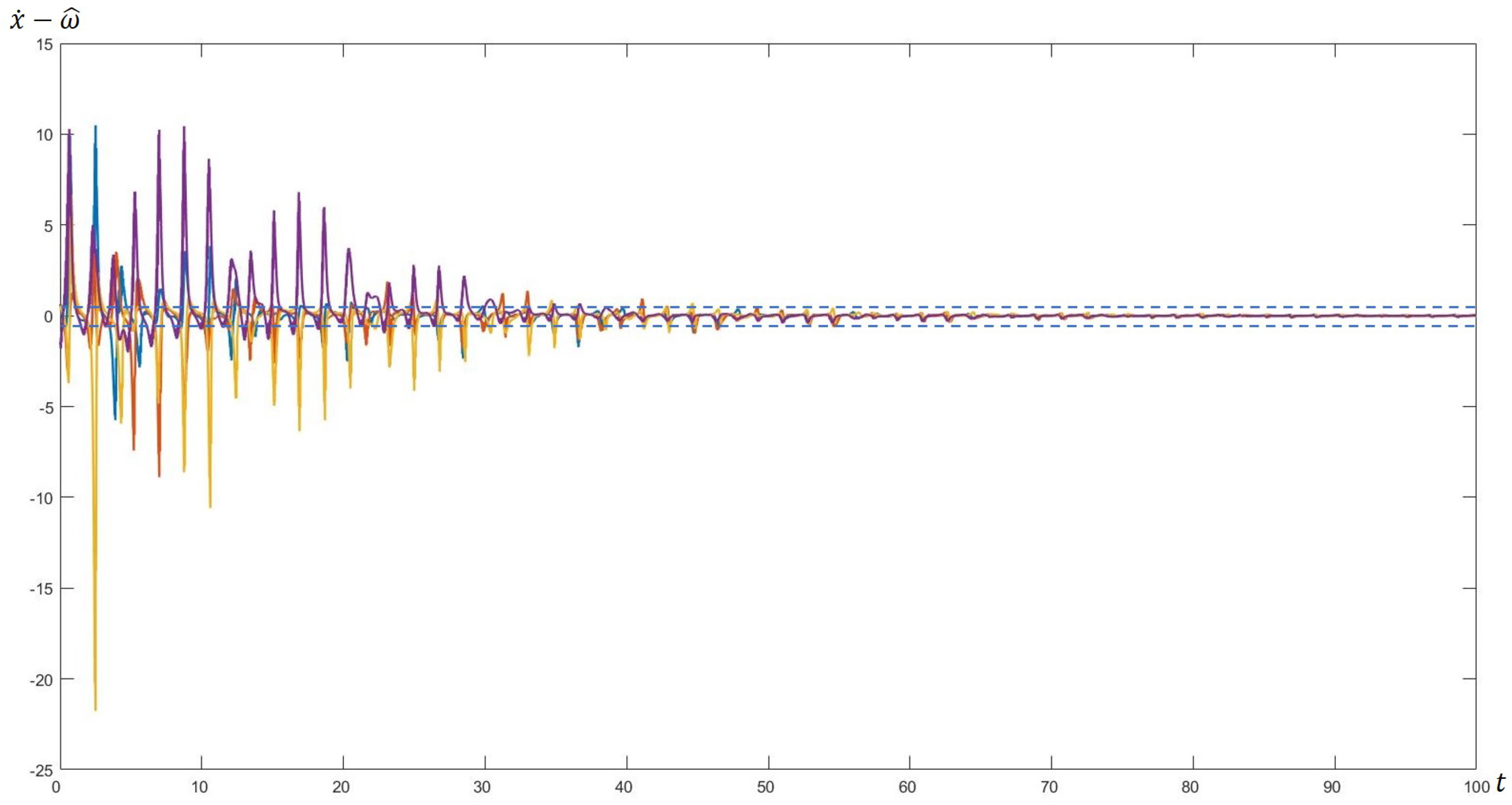
With such initial data, the system satisfies all the requirements from the list (1), and the dynamics of the state variables show an oscillatory behavior. The difference between the real output and its estimate at time $t_k$ is “forced into a stripe” (Figure 1) of width $2\Delta$ given by the inequalities (4) using the algorithm (8).

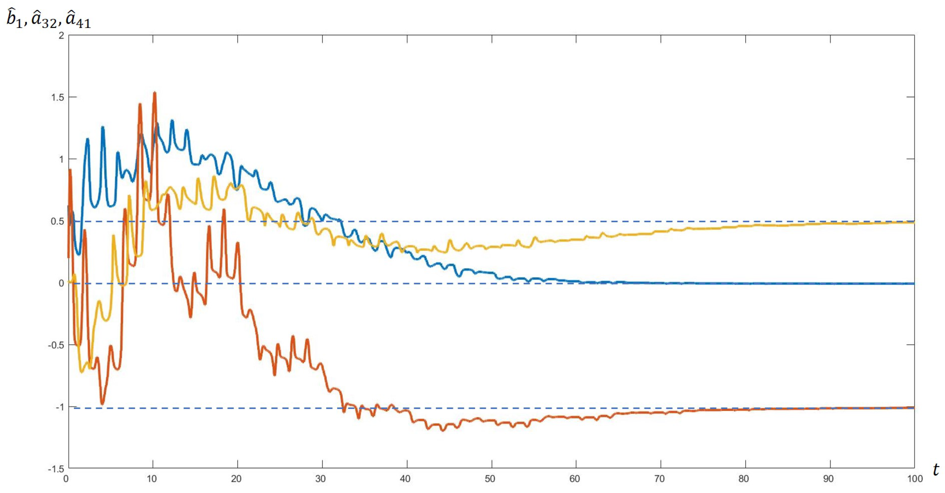
Parametric identification is performed and the adjusted coefficients are close to the reference values. Below is a comparison of all the estimates of the parameters defining the system with their real values (

Table 1. Comparison between $\theta$ and $\widehat{\theta }$.

b	$\widehat{\mathit{b}}$	A				$\widehat{\mathit{A}}$
0	−0.0048	0	2.2	−3.3	1.1	0.0025	2.1979	−3.3010	1.1010
−2	−2.0050	−2	0	0.5	3.5	−1.9990	0.023	0.4981	3.5011
−4.5	−4.4980	3	−0.5	0	2	3.0024	−0.4985	−0.0021	1.9981
6.5	6.4961	−1	−3.5	−2	0	−1.0013	−3.4994	−2.0017	0.0031

), as well as plots of how the estimates change over time (Figure 2) for three of them (taken arbitrarily as an example): ${\widehat{b}}_1,{\widehat{a}}_{32},{\widehat{a}}_{41}$.

Too large a number of measurements of the system state is not required for this approach. For identification of the system of the 4th order, 1000 measurements were enough. It may be possible to achieve this result with a smaller number of measurements. One of the ways in which this can be achieved will be described below.

If we know that matrix A of the model (1) is skew-symmetric, we can achieve higher speed and accuracy of the algorithm using this knowledge. It is quite reasonable to look for parameter estimates in the same form. The condition ${\widehat{a}}_{ij}=-{\widehat{a}}_{ji}$ can be satisfied by successively projecting the vector $\left[{\theta }_{1,k}^T,{\theta }_{2,k}^T,\dots {\theta }_{n,k}^T\right]\in R^{n\times n}$ onto the corresponding hyperplanes. A simple and fast algorithm is proposed for this purpose in the paper [21]. The composition of the algorithm from [21] and the algorithm (8) will still solve the system of inequalities (4) due to the fact that these algorithms satisfy the same Lyapunov function. The result of the modified algorithm is represented by the table (

Table 2. Comparison between $\theta$ and $\widehat{\theta }$.

b	$\widehat{\mathit{b}}$	A				$\widehat{\mathit{A}}$
0	0.0335	0	2	−3	1	0	1.9414	−2.9158	0.9862
−2	−1.9702	−2	0	0.5	3.5	−1.9414	0	0.5267	3.4335
−4.5	−4.4023	3	−0.5	0	2	2.9158	−0.5267	0	1.9706
6.5	6.3927	−1	−3.5	−2	0	−0.9862	−3.4335	−1.9706	0

) below.

Such modification of the algorithm according to the simulation results makes it possible to accelerate the convergence of the algorithm approximately by a factor of 1.2 for a 4th order system. For models of larger dimensions, it is natural to assume that the benefit of the modification will not be any less.

5.2. Parameter Identification under Noise in Dynamics and Measurements

One of the reasons why the Stripe algorithm is famous is its robustness to noise [15]. In the presentation of the theoretical results of this paper, neither interference in the measurement nor noise in the right-hand side of ordinary differential equations have been considered. This is a matter for future research. However, we will demonstrate by simulation that the research is reasonable, i.e., that the introduction of noise does not interfere with the algorithm (8).

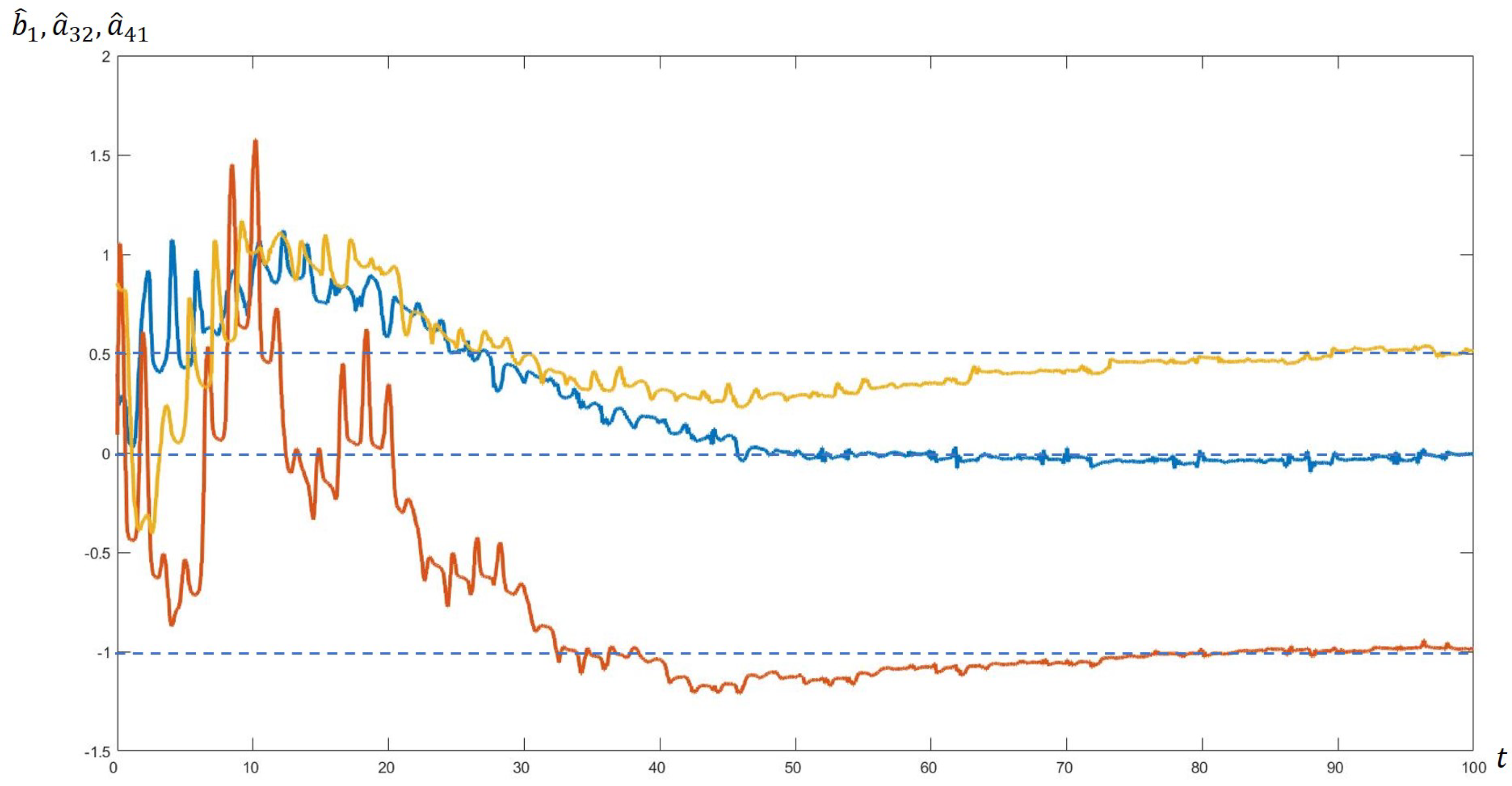
The initial data coincide with the case considered earlier

$$x\left(0\right)={[0.87,0.3,0.27,0.57]}^T,b={[0,-2,-4.5,6.5]}^T,A=\left[\begin{array}{cccc}0& 2.2& -3.3& 1.1\\ -2& 0& 0.5& 3.5\\ 3& -0.5& 0& 2\\ -1& -3.5& -2& 0\end{array}\right].$$

However, now the dynamics of the system has the form

$${\dot{x}}_i=x_i\left(b_i+\sum _{j=1}^n{a}_{ij}{x}_j\right)+s_i,i=1,\dots n,$$

where $s=s\left(t\right)$ is white noise with the bound $\left|s\right|<0.15$. In addition, instead of ${\dot{x}}_i$, a noisy signal is also fed to the input of the identification algorithm (Figure 3).

The graphs show that the introduction of various kinds of disturbances does not break the work of the identification algorithm.

It is easy to show using the results from [15] that the identification error grows in proportion to the amplitude of the measurement error (amplitude of the measurement noise). Modeling shows that the proportionality coefficient is small; for the given system it turns out to be approximately equal to $1/2$.

6. Conclusions

In this paper, we obtain the conditions under which the parameters of the generalized conservative Lotka-Volterra model (of any dimensionality) can be identified by the Stripe algorithm based on sampled data. Also in this paper, we obtain results for systems of general form. It is proved that if the recurrent trajectories are nonhyperplanar ones, it is sufficient to fulfill the persistent excitation condition. The validity of this statement holds when the data is given in a sampled form with a sufficiently small sampling interval. Persistent excitation condition arises in problems of identification theory very often, so these observations may be useful in future studies.

The presented theoretical results are illustrated by computer modeling. The modeling shows that results similar to those of the paper can be obtained for the case with noise in system dynamics and disturbances in state variables measurements. Also significant is the question of the convergence rate of the algorithm for identifying the parameters of the Lotka-Volterra model. The authors hope that research will continue in directions related to the results of this article.