


A Novel Method for Medical Predictive Models in Small Data Using Out-of-Distribution Data and Transfer Learning


Abstract
1. Introduction
- Introducing a highly intuitive and simple idea and assessing the potential utility of OOD data in creating pre-trained models for TL.
- Experimentally validating the effectiveness of OOD and TL in small medical datasets while minimizing artificial data manipulations, such as data generation.
- Developing a predictive model for ARF in patients with acute pesticide poisoning using the proposed method, showcasing low bias and high performance.
2. Materials and Methods
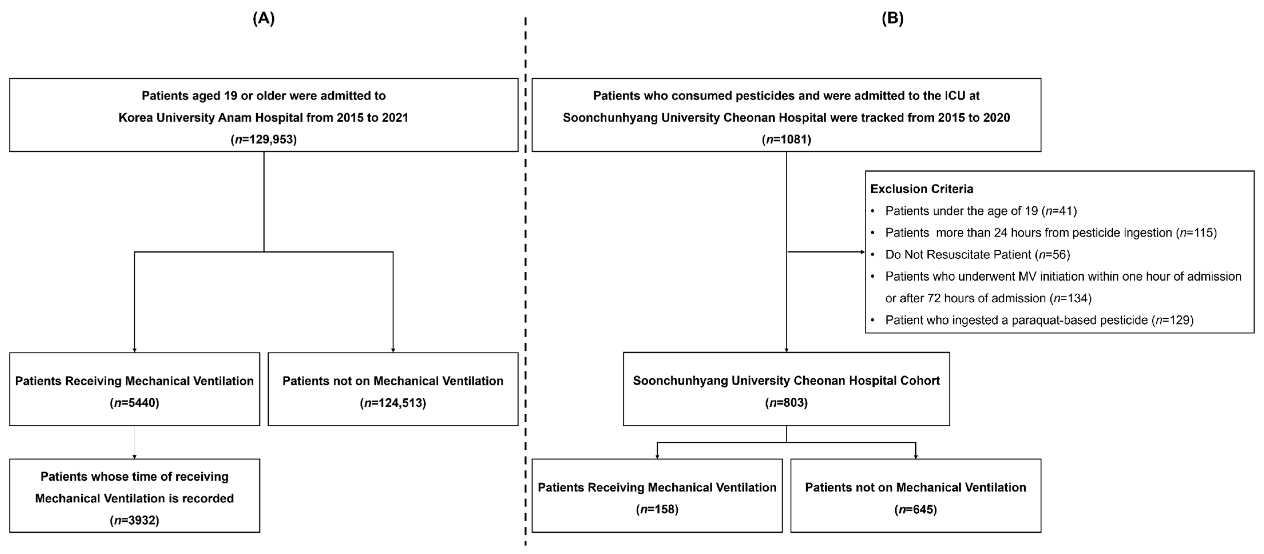
2.1. Study Population
2.2. Labeling
2.3. Feature Selection
2.4. Handling of Outliers and Missing Values
2.5. Modeling and Performance Evaluation
2.6. Statistical Analysis and Model Interpretation
3. Results
3.1. Study Participants’ Characteristics
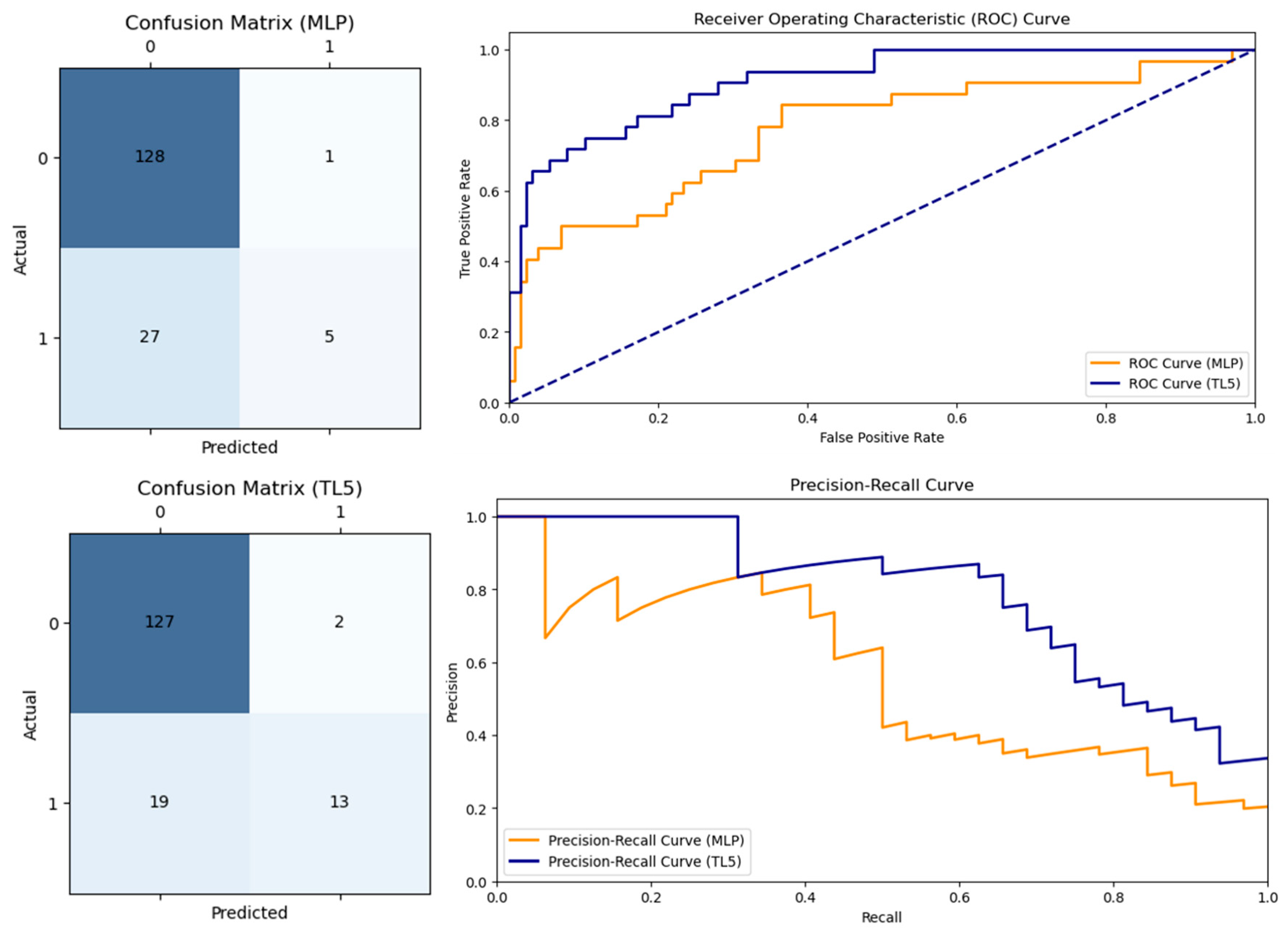
3.2. Model Performance
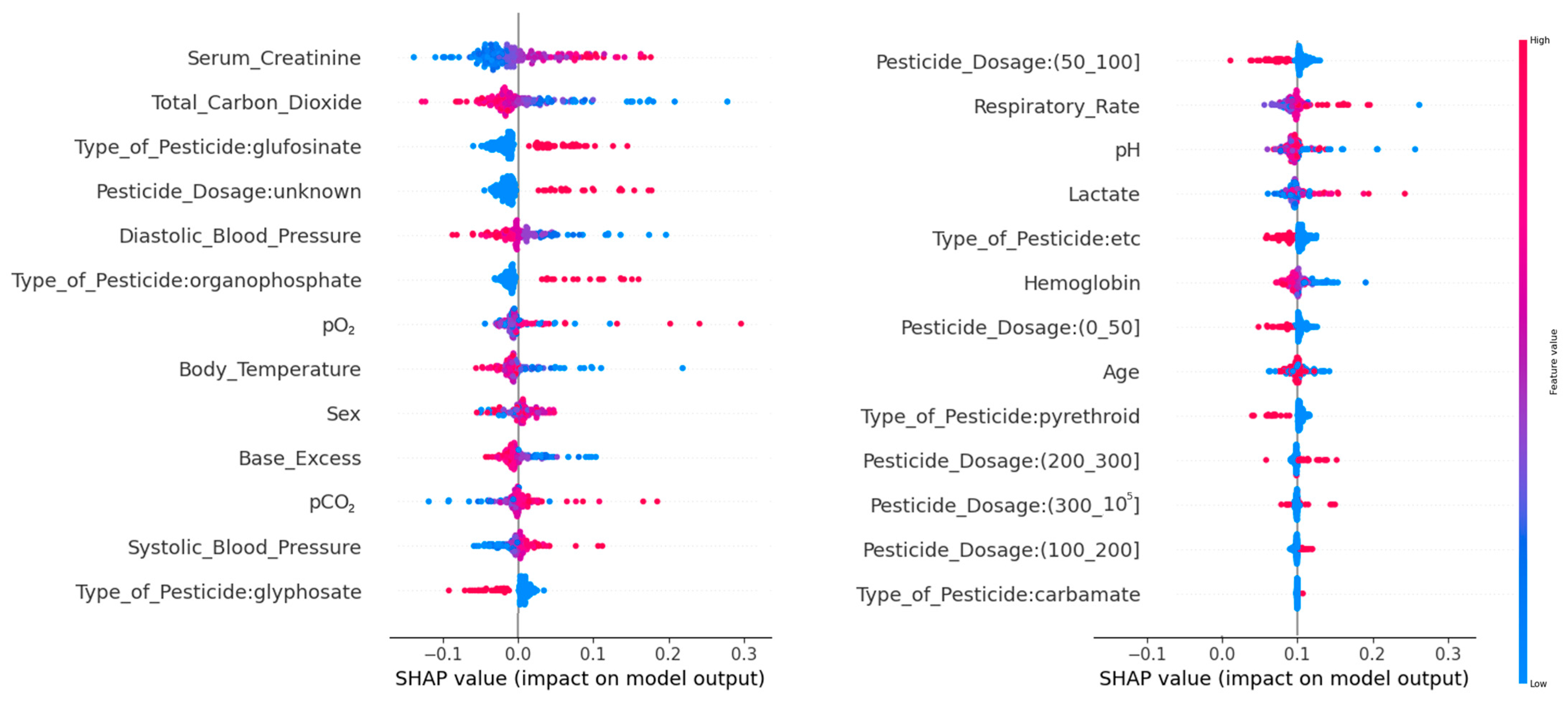
3.3. Model Interpretation
- High Cr, low TCO2 and low DBP significantly contributed to the development of ARF.
- Older age, low BE, high pCO2 and high SBP may contribute to the development of ARF.
- Glufosinate and organophosphates were more likely to contribute to the development of ARF than other pesticides.
- Ingesting less than 100 cc carried a lower likelihood of developing ARF, while those who ingested 100–200 cc showed higher likelihood.
4. Discussion
5. Conclusions
Author Contributions
Funding
Data Availability Statement
Acknowledgments
Conflicts of Interest
Appendix A


| Category | Abbreviation | Full Form |
|---|---|---|
| Model | LGBM | Light Gradient-Boosting Machine |
| LR | Logistic Regression | |
| MLP | Multi-Layer Perceptron | |
| RF | Random Forest | |
| XGB | Extreme Gradient Boosting | |
| Metrics | AUROC | Area Under the Receiver Operating Characteristic |
| AUPRC | Area Under the Precision–Recall Curve | |
| MCC | Matthews Correlation Coefficient | |
| SHAP | ShaHley Additive exPlanations | |
| Features | BE | Base Excess |
| DBP | Diastolic Blood Pressure | |
| GCS | Glasgow Coma Scale | |
| SBP | Systolic Blood Pressure | |
| Total CO2 | Total Carbon Dioxide | |
| ETC | ARF | Acute Respiratory Failure |
| DL | Deep Learning | |
| EHR | Electronic Health Records | |
| IRB | Institutional Review Boards | |
| MICE | Multiple Imputation by Chained Equations | |
| MV | Mechanical Ventilation | |
| OOD | Out-of-Distribution | |
| TL | Transfer Learning |
| Feature | Korea University Anam Hospital (n = 12,059) | Soonchunhyang University Cheonan Hospital (n = 803) | ||
|---|---|---|---|---|
| N | % | N | % | |
| Age | 0 | 0.00 | 0 | 0.00 |
| Sex 1 | 0 | 0.00 | 0 | 0.00 |
| Systolic BP 2 | 53,138 | 19.61 | 22 | 2.74 |
| Diastolic BP | 52,928 | 19.53 | 29 | 3.61 |
| Respiratory | 14,632 | 5.40 | 27 | 3.36 |
| Heart rate | 13,648 | 5.04 | 38 | 4.73 |
| Serum Cr 3 | 14,047 | 5.18 | 28 | 3.49 |
| Hemoglobin | 13,172 | 4.86 | 41 | 5.11 |
| Total CO2 | 11,695 | 4.32 | 65 | 8.09 |
| Arterial pH | 13,024 | 4.81 | 43 | 5.35 |
| pCO2 | 13,307 | 4.91 | 39 | 4.86 |
| pO2 | 13,531 | 4.99 | 43 | 5.35 |
| BE 4 | 13,421 | 4.95 | 43 | 5.35 |
| Lactate | 10,295 | 3.80 | 50 | 6.23 |
| GCS 5 | 251,420 | 92.78 | 24 | 2.99 |
| Feature | N | % |
|---|---|---|
| Pesticide category | ||
| Not otherwise specified | 227 | 28.27 |
| Glyphosate | 213 | 26.53 |
| Glufosinate | 186 | 23.16 |
| Organophosphate | 90 | 11.21 |
| Pyrethroid | 78 | 9.71 |
| Carbamate | 9 | 1.12 |
| Amount of ingestion | ||
| ≤50 cc | 168 | 20.92 |
| >50 cc, ≤100 cc | 160 | 19.93 |
| >100 cc, ≤200 cc | 157 | 19.55 |
| >200 cc, ≤300 cc | 131 | 16.31 |
| >300 cc | 97 | 12.08 |
| Unknown | 90 | 11.21 |
| Model | AUROC | F1 | ||
|---|---|---|---|---|
| Mean | 95% CI | Mean | 95% CI | |
| LR | 0.9076 | 0.8872–0.9279 | 0.6800 | 0.5946–0.7655 |
| RF | 0.9115 | 0.8687–0.9544 | 0.5783 | 0.5106–0.6460 |
| XGB | 0.9039 | 0.8695–0.9383 | 0.6316 | 0.5459–0.7174 |
| LGBM | 0.9056 | 0.8966–0.9146 | 0.6339 | 0.5401–0.7277 |
| MLP | 0.8842 | 0.8460–0.9225 | 0.6321 | 0.4985–0.7658 |
Appendix B
- Pima Indian: Smith, J.W., Everhart, J.E., Dickson, W.C., Knowler, W.C., & Johannes, R.S. (1988). https://www.kaggle.com/datasets/uciml/pima-indians-diabetes-database (accessed on 1 January 2024).
- Cirrhosis Patient Survival Prediction: Dickson, E., Grambsch, P., Fleming, T., Fisher, L., and Langworthy, A. (2023). Cirrhosis Patient Survival Prediction. UCI Machine Learning Repository. https://doi.org/10.24432/C5R02G.
- NHANES: National Health and Nutrition Health Survey 2013–2014 (NHANES) (2023) Age Prediction Subset. UCI Machine Learning Repository. https://doi.org/10.24432/C5BS66.
- Wisconsin Breast Cancer: Wolberg, William, Mangasarian, Olvi, Street, Nick, and Street, W. (1995). Breast Cancer Wisconsin (Diagnostic). UCI Machine Learning Repository. https://doi.org/10.24432/C5DW2B.
- Parkinsons Telemonitoring: Tsanas, Athanasios and Little, Max. (2009). Parkinsons Telemonitoring. UCI Machine Learning Repository. https://doi.org/10.24432/C5ZS3N.
- CDC Diabetes Health Indicators: This dataset was released by the CDC. https://doi.org/10.24432/C53919.
| Feature | BMI ≥ 25 (N = 651) | BMI < 25 (N = 117) | p-Value |
|---|---|---|---|
| Glucose | 123.36 ± 32.29 | 107.20 ± 26.31 | <0.0001 * |
| Blood pressure | 70.49 ± 18.02 | 61.39 ± 24.21 | 0.0002 * |
| Skin thickness | 22.48 ± 16.06 | 9.71 ± 9.90 | <0.0001 * |
| Insulin | 86.90 ± 120.25 | 40.28 ± 70.27 | <0.0001 * |
| DPF | 0.48 ± 0.33 | 0.41 ± 0.31 | 0.0220 * |
| Age | 33.56 ± 11.44 | 31.49 ± 13.34 | 0.1170 |
| Pregnancies | 3.0 (1.0, 6.0) | 2.0 (1.0, 5.0) | 0.0401 * |

| Feature | Dataset for Pre-Training | Dataset for Fine-Tuning | p-Value |
|---|---|---|---|
| Female (N = 368) | Male (N = 44) | ||
| D-penicillamine | 137 (37.23) | 21 (47.73) | 0.2342 |
| Ascites | 21 (5.71) | 3 (6.82) | 1.0000 |
| Hepatomegaly | 139 (37.77) | 21 (47.73) | 0.2640 |
| Spiders | 86 (23.37) | 4 (9.09) | 0.0485 * |
| Edema | 56 (15.22) | 8 (18.18) | 0.7696 |
| Age | 50.07 ± 10.25 | 55.75 ± 11.00 | 0.0020 * |
| Bilirubin | 3.27 ± 4.62 | 2.87 ± 2.32 | 0.3426 |
| Cholesterol | 370.50 ± 238.73 | 362.46 ± 178.99 | 0.8129 |
| Albumin | 3.50 ± 0.42 | 3.53 ± 0.46 | 0.5906 |
| Copper | 90.21 ± 80.74 | 154.28 ± 100.67 | 0.0007 * |
| Alk_Phos | 1957.83 ± 2105.05 | 2172.95 ± 2418.45 | 0.6133 |
| SGOT | 122.63 ± 57.92 | 121.99 ± 47.01 | 0.9408 |
| Tryglicerides | 123.47 ± 66.78 | 133.43 ± 52.17 | 0.3135 |
| Platelets | 259.10 ± 96.61 | 231.14 ± 85.23 | 0.0501 |
| Prothrombin | 10.71 ± 1.04 | 10.94 ± 0.93 | 0.1280 |
| Age < 60 (N = 324) | Age ≥ 60 (N = 88) | ||
| D-penicillamine | 120 (37.04) | 38 (43.18) | 0.3536 |
| Male | 27 (8.33) | 17 (19.32) | 0.0057 * |
| Ascites | 13 (4.01) | 11 (12.50) | 0.0058 * |
| Hepatomegaly | 126 (38.89) | 34 (38.64) | 1.0000 |
| Spiders | 77 (23.77) | 13 (14.77) | 0.0959 |
| Edema | 39 (12.04) | 25 (28.41) | 0.0003 * |
| Bilirubin | 3.33 ± 4.65 | 2.86 ± 3.51 | 0.3086 |
| Cholesterol | 379.49 ± 248.56 | 327.96 ± 137.49 | 0.0392 * |
| Albumin | 3.52 ± 0.42 | 3.41 ± 0.43 | 0.0349* |
| Copper | 96.84 ± 86.91 | 101.07 ± 80.47 | 0.7218 |
| Alk_Phos | 2008.02 ± 2174.57 | 1876.12 ± 2004.30 | 0.6534 |
| SGOT | 124.48 ± 57.91 | 114.48 ± 50.97 | 0.1868 |
| Tryglicerides | 123.84 ± 64.71 | 128.27 ± 67.43 | 0.6603 |
| Platelets | 260.10 ± 97.20 | 241.24 ± 89.15 | 0.0916 |
| Prothrombin | 10.68 ± 0.99 | 10.92 ± 1.15 | 0.0748 |
| Placebo (N = 254) | D-penicillamine (N = 158) | ||
| Male | 23 (9.06) | 21 (13.29) | 0.2342 |
| Ascites | 10 (3.94) | 14 (8.86) | 0.0631 |
| Hepatomegaly | 87 (34.25) | 73 (46.20) | 0.0206 * |
| Spiders | 45 (17.72) | 45 (28.48) | 0.0143 * |
| Edema | 38 (14.96) | 26 (16.46) | 0.7891 |
| Age | 50.18 ± 10.10 | 51.47 ± 11.01 | 0.2324 |
| Bilirubin | 3.45 ± 4.86 | 2.87 ± 3.63 | 0.1717 |
| Cholesterol | 373.88 ± 252.48 | 365.01 ± 209.54 | 0.7474 |
| Albumin | 3.49 ± 0.41 | 3.52 ± 0.44 | 0.5485 |
| Copper | 97.65 ± 80.49 | 97.64 ± 90.59 | 0.9992 |
| Alk_Phos | 1943.01 ± 2101.69 | 2021.30 ± 2183.44 | 0.7471 |
| SGOT | 124.97 ± 58.93 | 120.21 ± 54.52 | 0.4602 |
| Tryglicerides | 125.25 ± 58.52 | 124.14 ± 71.54 | 0.8864 |
| Platelets | 254.42 ± 92.89 | 258.75 ± 100.32 | 0.6646 |
| Prothrombin | 10.78 ± 1.12 | 10.65 ± 0.85 | 0.1829 |

| Feature | No Diabetes (N = 2198) | Suspected Diabetes (N = 79) | p-Value |
|---|---|---|---|
| Female | 1127 (51.27) | 38 (48.10) | 0.6631 |
| Regular moderate-to-high-intensity exercise | 1808 (82.26) | 60 (75.95) | 0.1986 |
| BMI | 27.83 ± 7.17 | 31.43 ± 8.56 | 0.0004 * |
| Glucose | 98.63 ± 14.25 | 125.34 ± 54.05 | <0.0001 * |
| 2-h OGTT glucose | 112.61 ± 42.54 | 180.85 ± 95.45 | <0.0001 * |
| Insulin | 11.66 ± 9.46 | 16.57 ± 14.53 | 0.0039 * |

| Feature | Cluster 1 (N = 445) | Cluster 0 (N = 124) | p-Value |
|---|---|---|---|
| Radius | 12.60 ± 1.92 | 19.62 ± 2.27 | <0.0001 * |
| Texture | 18.58 ± 4.10 | 21.84 ± 4.03 | <0.0001 * |
| Perimeter | 81.45 ± 13.18 | 129.71 ± 16.23 | <0.0001 * |
| Area | 499.67 ± 149.85 | 1211.94 ± 301.41 | <0.0001 * |
| Smoothness | 0.0953 ± 0.0144 | 0.1003 ± 0.0122 | 0.0001 * |
| Compactness | 0.0928 ± 0.0460 | 0.1459 ± 0.0549 | <0.0001 * |
| Concavity | 0.0645 ± 0.0603 | 0.1760 ± 0.0802 | <0.0001 * |
| Concave points | 0.0346 ± 0.0251 | 0.1003 ± 0.0356 | <0.0001 * |
| Symmetry | 0.1787 ± 0.0264 | 0.1901 ± 0.0292 | 0.0001 * |
| Fractal dimension | 0.0636 ± 0.0070 | 0.0599 ± 0.0064 | <0.0001 * |
| Feature | Age > 60 (N = 27) | Age ≤ 60 (N = 15) | p-Value |
|---|---|---|---|
| Female | 8 (29.63) | 6 (40.00) | 0.7327 |
| Motor UPDRS | 22.93 ± 8.07 | 18.21 ± 7.31 | <0.0001 * |
| Jitter (%) | 0.006568 ± 0.005735 | 0.005370 ± 0.005323 | <0.0001 * |
| Jitter (Abs) | 0.000047 ± 0.000037 | 0.000039 ± 0.000033 | <0.0001 * |
| Jitter: RAP | 0.003184 ± 0.003134 | 0.002615 ± 0.003072 | <0.0001 * |
| Jitter: PPQ5 | 0.003554 ± 0.004008 | 0.002752 ± 0.003078 | <0.0001 * |
| Jitter: DDP | 0.009552 ± 0.009401 | 0.007846 ± 0.009215 | <0.0001 * |
| Shimmer | 0.038 ± 0.028 | 0.027 ± 0.019 | <0.0001 * |
| Shimmer (dB) | 0.344 ± 0.252 | 0.249 ± 0.166 | <0.0001 * |
| Shimmer: APQ3 | 0.019 ± 0.014 | 0.014 ± 0.010 | <0.0001 * |
| Shimmer: APQ5 | 0.022 ± 0.018 | 0.016 ± 0.012 | <0.0001 * |
| Shimmer: APQ11 | 0.030 ± 0.021 | 0.022 ± 0.016 | <0.0001 * |
| Shimmered | 0.057 ± 0.043 | 0.042 ± 0.030 | <0.0001 * |
| NHR | 0.037 ± 0.070 | 0.023 ± 0.030 | <0.0001 * |
| HNR | 21.21 ± 4.29 | 22.56 ± 4.16 | <0.0001 * |
| RPDE | 0.55 ± 0.09 | 0.52 ± 0.11 | <0.0001 * |
| DFA | 0.64 ± 0.07 | 0.67 ± 0.07 | <0.0001 * |
| PPE | 0.23 ± 0.09 | 0.20 ± 0.08 | <0.0001 * |
| Metrics | Without TL | With TL | ||
|---|---|---|---|---|
| Mean | 95% CI | Mean | 95% CI | |
| MSE | 34.08 | 31.54–35.61 | 33.40 | 30.55–36.25 |
| R2 | 0.36 | 0.28–0.45 | 0.42 | 0.35–0.49 |

| Feature | Dataset for Pre-Training | Dataset for Fine-Tuning | p-Value |
|---|---|---|---|
| No Stroke (N = 243,388) | Stroke (N = 10,292) | ||
| HighBP | 101,204 (41.58) | 7625 (74.09) | <0.0001 * |
| HighChol | 100,935 (41.47) | 6656 (64.67) | <0.0001 * |
| Smoke | 106,341 (43.69) | 6082 (59.09) | <0.0001 * |
| CHD | 19,956 (8.20) | 3937 (38.25) | <0.0001 * |
| PhysActivity | 185,619 (76.26) | 6301 (61.22) | <0.0001 * |
| Fruits | 154,693 (63.56) | 6205 (60.29) | <0.0001 * |
| Veggies | 198,295 (81.47) | 7546 (73.32) | <0.0001 * |
| Binge drinker | 13,873 (5.70) | 383 (3.72) | <0.0001 * |
| GenHlth | <0.0001 * | ||
| Excellent | 44,854 (18.43) | 445 (4.32) | |
| Very good | 87,420 (35.92) | 1664 (16.17) | |
| Good | 72,473 (29.78) | 3173 (30.83) | |
| Fair | 28,591 (11.75) | 2979 (28.94) | |
| Poor | 10,050 (4.13) | 2031 (19.73) | |
| DiffWalk | 37,638 (15.46) | 5037 (48.94) | <0.0001 * |
| Male | 107,100 (44.00) | 4606 (44.75) | 0.1362 |
| Age ≥ 60 | 114,696 (47.12) | 7618 (74.02) | <0.0001 * |
| BMI | 28.35 ± 6.59 | 29.03 ± 6.94 | <0.0001 * |
| No CHD (N = 229,787) | CHD (N = 23,893) | ||
| HighBP | 90,901 (39.56) | 17,928 (75.03) | <0.0001 * |
| HighChol | 90,838 (39.53) | 16,753 (70.12) | <0.0001 * |
| Smoke | 97,622 (42.48) | 14,801 (61.95) | <0.0001 * |
| Stroke | 6355 (2.77) | 3937 (16.48) | <0.0001 * |
| PhysActivity | 176,620 (76.86) | 15,300 (64.04) | <0.0001 * |
| Fruits | 146,450 (63.73) | 14,448 (60.47) | <0.0001 * |
| Veggies | 187,589 (81.64) | 18,252 (76.39) | <0.0001 * |
| Binge drinker | 13,408 (5.83) | 848 (3.55) | <0.0001 * |
| GenHlth | <0.0001 * | ||
| Excellent | 44,283 (19.27) | 1016 (4.25) | |
| Very good | 84,956 (36.97) | 4128 (17.28) | |
| Good | 67,732 (29.48) | 7914 (33.12) | |
| Fair | 24,842 (10.81) | 6728 (28.16) | |
| Poor | 7974 (3.47) | 4107 (17.19) | |
| DiffWalk | 32,760 (14.26) | 9915 (41.5) | <0.0001 * |
| Male | 98,018 (42.66) | 13,688 (57.29) | <0.0001 * |
| Age ≥ 60 | 103,564 (45.07) | 18,750 (78.47) | <0.0001 * |
| BMI | 28.27 ± 6.58 | 29.47 ± 6.74 | <0.0001 * |
| Non-binge drinker (N = 239,424) | Binge drinker (N = 14,256) | ||
| HighBP | 102,828 (42.95) | 6001 (42.09) | 0.0464 * |
| HighChol | 101,878 (42.55) | 5713 (40.07) | <0.0001 * |
| Smoke | 103,156 (43.09) | 9267 (65.0) | <0.0001 * |
| Stroke | 9909 (4.14) | 383 (2.69) | <0.0001 * |
| CHD | 23,045 (9.63) | 848 (5.95) | <0.0001 * |
| PhysActivity | 180,824 (75.52) | 11,096 (77.83) | <0.0001 * |
| Fruits | 152,849 (63.84) | 8049 (56.46) | <0.0001 * |
| Veggies | 193,792 (80.94) | 12,049 (84.52) | <0.0001 * |
| GenHlth | <0.0001 * | ||
| Excellent | 42,346 (17.69) | 2953 (20.71) | |
| Very good | 83,618 (34.92) | 5466 (38.34) | |
| Good | 71,515 (29.87) | 4131 (28.98) | |
| Fair | 30,272 (12.64) | 1298 (9.10) | |
| Poor | 11,673 (4.88) | 408 (2.86) | |
| DiffWalk | 41,100 (17.17) | 1575 (11.05) | <0.0001 * |
| Male | 105,262 (43.96) | 6444 (45.20) | 0.0039 * |
| Age ≥ 60 | 116,324 (48.58) | 5990 (42.02) | <0.0001 * |
| BMI | 28.46 ± 6.65 | 27.06 ± 5.79 | <0.0001 * |
| Dataset | Metrics | Without TL | With TL | |||
|---|---|---|---|---|---|---|
| Mean | 95% CI | Mean | 95% CI | |||
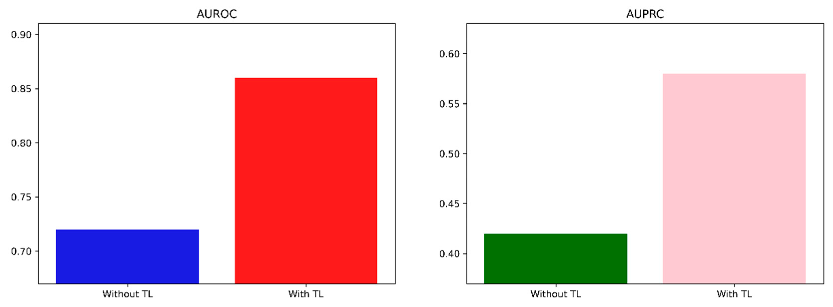
| Pima Indian | AUROC | 0.72 | 0.69–0.74 | 0.86 | 0.85–0.87 | |
| AUPRC | 0.42 | 0.40–0.45 | 0.58 | 0.55–0.60 | ||
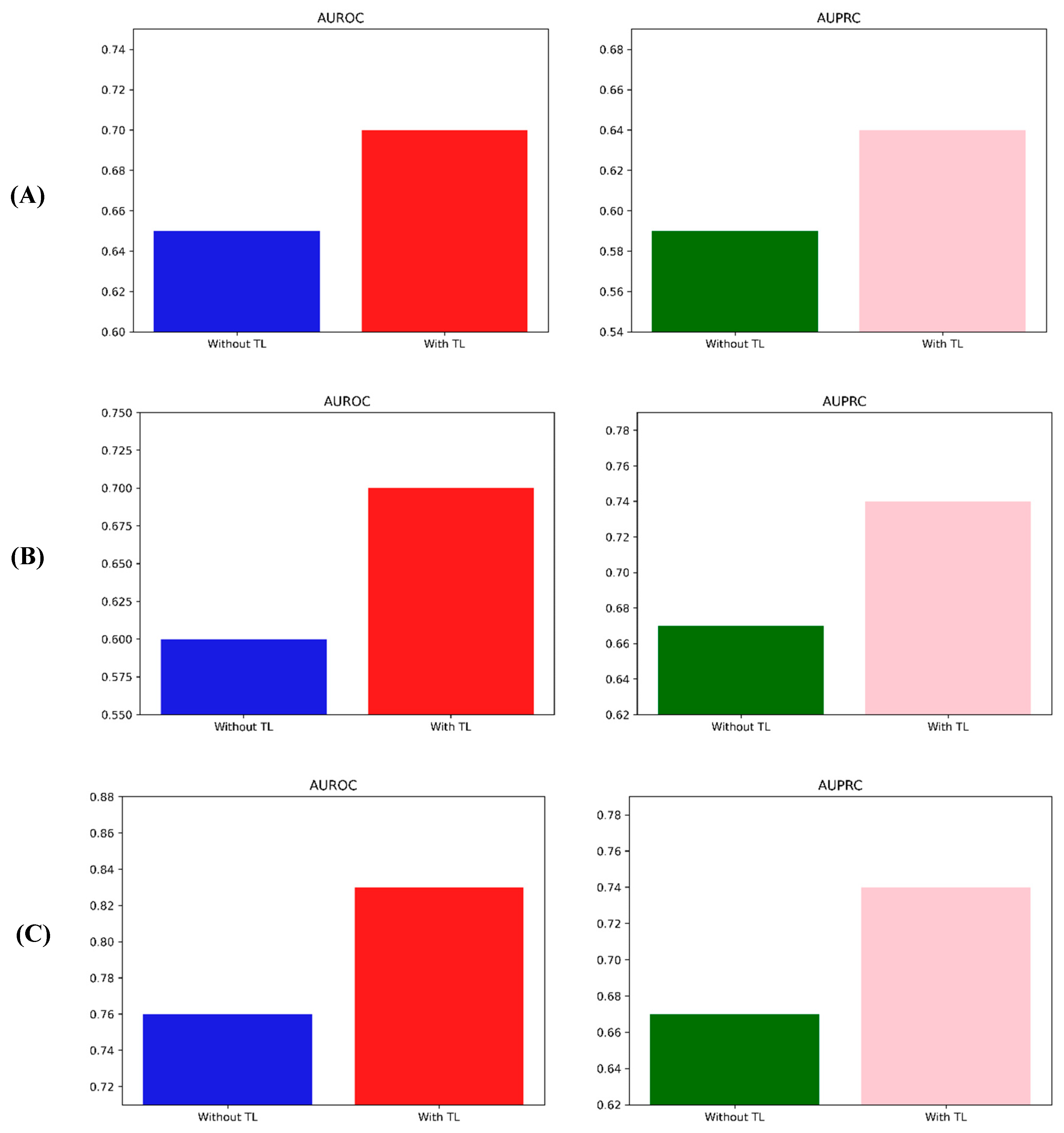
| Cirrhosis Patient Survival Prediction | Male | AUROC | 0.65 | 0.63–0.66 | 0.70 | 0.69–0.72 |
| AUPRC | 0.59 | 0.57–0.61 | 0.64 | 0.63–0.66 | ||
| Elderly | AUROC | 0.60 | 0.59–0.61 | 0.70 | 0.69–0.71 | |
| AUPRC | 0.67 | 0.66–0.68 | 0.74 | 0.73–0.75 | ||
| D-penicillamine | AUROC | 0.76 | 0.75–0.78 | 0.83 | 0.82–0.84 | |
| AUPRC | 0.67 | 0.66–0.69 | 0.74 | 0.73–0.75 | ||
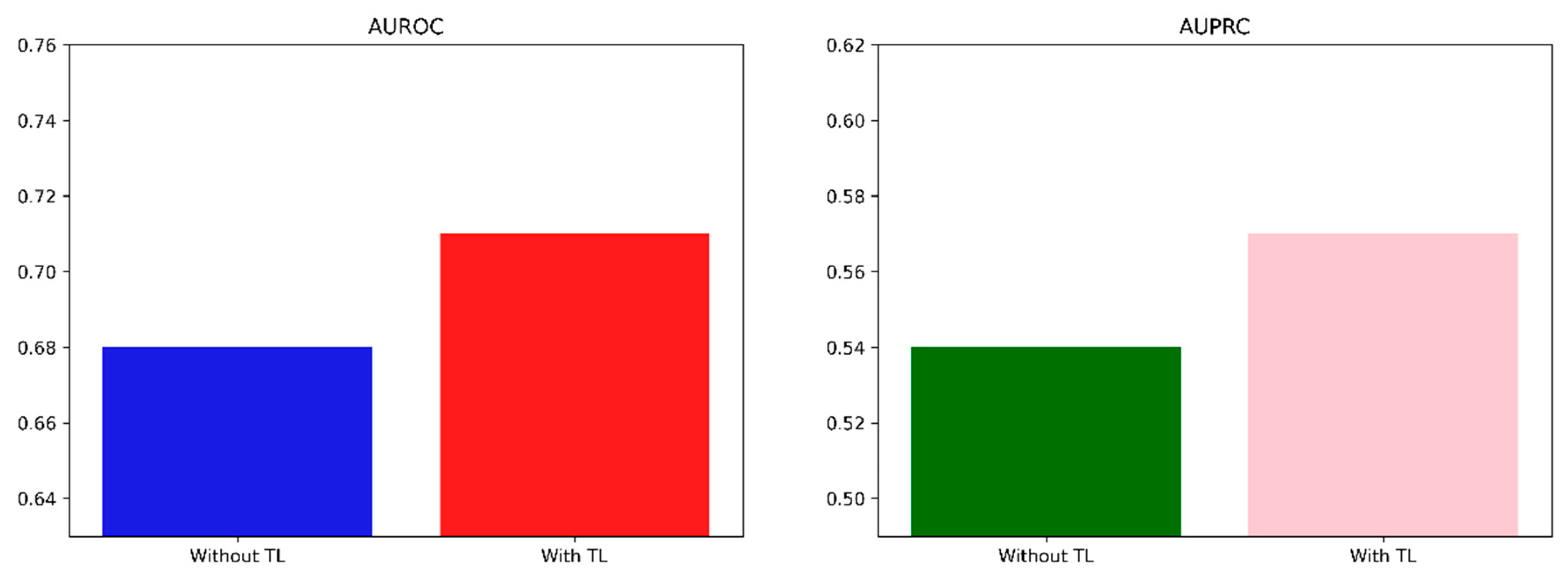
| NHANES | AUROC | 0.68 | 0.67–0.69 | 0.71 | 0.70–0.72 | |
| AUPRC | 0.54 | 0.52–0.55 | 0.57 | 0.56–0.59 | ||
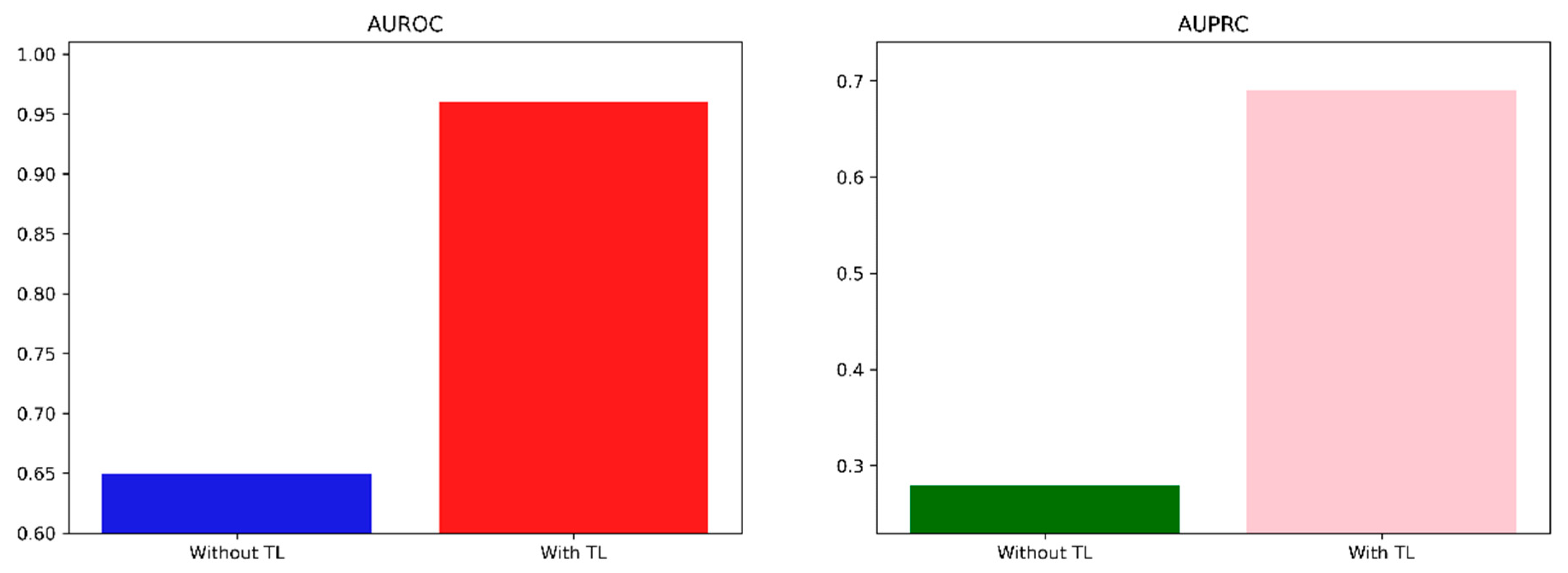
| Wisconsin Breast Cancer | AUROC | 0.65 | 0.61–0.69 | 0.96 | 0.95–0.97 | |
| AUPRC | 0.28 | 0.25–0.32 | 0.69 | 0.65–0.73 | ||
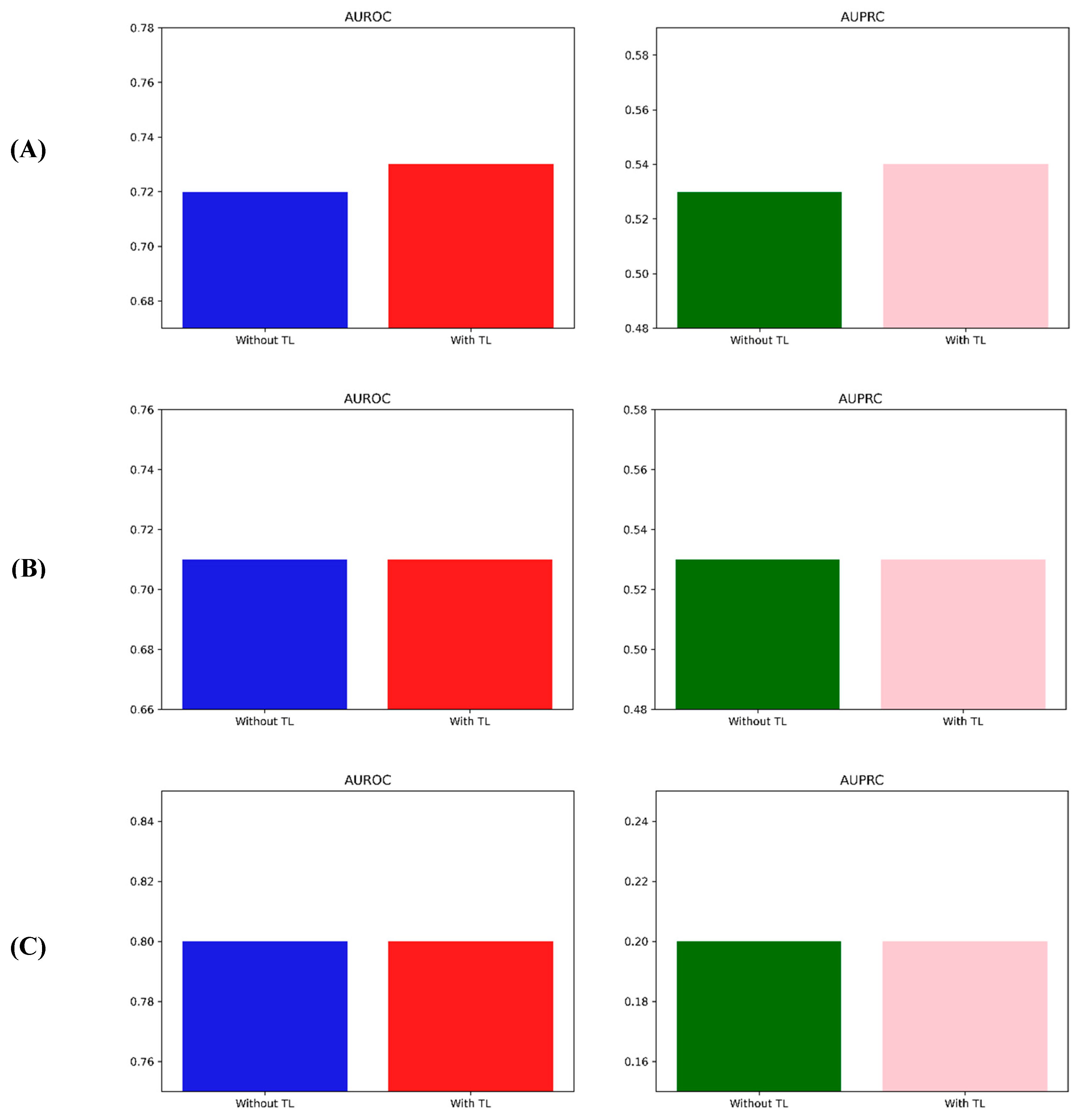
| CDC Diabetes Health Indicators | Stroke | AUROC | 0.72 | 0.72–0.72 | 0.73 | 0.73–0.73 |
| AUPRC | 0.53 | 0.53–0.54 | 0.54 | 0.54–0.55 | ||
| CHD | AUROC | 0.71 | 0.71–0.71 | 0.71 | 0.71–0.71 | |
| AUPRC | 0.53 | 0.53–0.53 | 0.53 | 0.53–0.53 | ||
| Binge drinker | AUROC | 0.80 | 0.80–0.80 | 0.80 | 0.80–0.80 | |
| AUPRC | 0.20 | 0.19–0.20 | 0.20 | 0.19–0.20 | ||
References
- Alzubaidi, L.; Zhang, J.; Humaidi, A.J.; Al-Dujaili, A.; Duan, Y.; Al-Shamma, O.; Santamaría, J.; Fadhel, M.A.; Al-Amidie, M.; Farhan, L. Review of deep learning: Concepts, CNN architectures, challenges, applications, future directions. J. Big Data 2021, 8, 53. [Google Scholar] [CrossRef] [PubMed]
- Lateh, M.A.; Muda, A.K.; Yusof, Z.I.M.; Muda, N.A.; Azmi, M.S. Handling a small dataset problem in prediction model by employ artificial data generation approach: A review. J. Phys. Conf. Ser. 2017, 892, 012016. [Google Scholar] [CrossRef]
- Vapnik, V. The Nature of Statistical Learning Theory; Springer Science & Business Media: Berlin/Heidelberg, Germany, 1999. [Google Scholar]
- Andonie, R. Extreme data mining: Inference from small datasets. Int. J. Comput. Commun. Control 2010, 5, 280–291. [Google Scholar] [CrossRef]
- Tsai, T.I.; Li, D.C. Utilize bootstrap in small data set learning for pilot run modeling of manufacturing systems. Expert Syst. Appl. 2008, 35, 1293–1300. [Google Scholar] [CrossRef]
- Niyogi, P.; Girosi, F.; Poggio, T. Incorporating prior information in machine learning by creating virtual examples. Proc. IEEE 1998, 86, 2196–2209. [Google Scholar] [CrossRef]
- Chao, G.; Tsai, T.; Lu, T.-J.; Hsu, H.; Bao, B.; Wu, W.; Lin, M.; Lu, T. A new approach to prediction of radiotherapy of bladder cancer cells in small dataset analysis. Expert Syst. Appl. 2011, 38, 7963–7969. [Google Scholar] [CrossRef]
- Da Silva, I.B.V.; Adeodato, P.J. PCA and Gaussian noise in MLP neural network training improve generalization in problems with small and unbalanced data sets. In Proceedings of the 2011 International Joint Conference on Neural Networks, San Jose, CA, USA, 31 July–5 August 2011; IEEE: New York, NY, USA, 2011; pp. 2664–2669. [Google Scholar]
- Karimi, D.; Gholipour, A. Improving calibration and out-of-distribution detection in deep models for medical image segmentation. IEEE Trans. Artif. Intell. 2022, 4, 383–397. [Google Scholar] [CrossRef]
- Major, D.; Lenis, D.; Wimmer, M.; Berg, A.; Neubauer, T.; Bühler, K. On the importance of domain awareness in classifier interpretations in medical imaging. IEEE Trans. Med. Imag. 2023, 42, 2286–2298. [Google Scholar] [CrossRef]
- Dodge, J.; Ilharco, G.; Schwartz, R.; Farhadi, A.; Hajishirzi, H.; Smith, N. Fine-tuning pretrained language models: Weight initializations, data orders, and early stopping. arXiv 2020, arXiv:2002.06305. [Google Scholar]
- Narkhede, M.V.; Bartakke, P.P.; Sutaone, M.S. A review on weight initialization strategies for neural networks. Artif. Intell. Rev. 2022, 55, 291–322. [Google Scholar] [CrossRef]
- Izonin, I.; Roman, T. Universal intraensemble method using nonlinear AI techniques for regression modeling of small medical data sets. In Cognitive and Soft Computing Techniques for the Analysis of Healthcare Data; Academic Press: Cambridge, MA, USA, 2022; pp. 123–150. [Google Scholar]
- Hekler, E.B.; Klasnja, P.; Chevance, G.; Golaszewski, N.M.; Lewis, D.; Sim, I. Why we need a small data paradigm. BMC Med. 2019, 17, 133. [Google Scholar] [CrossRef]
- Li, D.-C.; Wu, C.-S.; Tsai, T.-I.; Chang, F.M. Using mega-fuzzification and data trend estimation in small data set learning for early FMS scheduling knowledge. Comput. Oper. Res. 2006, 33, 1857–1869. [Google Scholar] [CrossRef]
- Shorten, C.; Khoshgoftaar, T.M. A survey on image data augmentation for deep learning. J. Big Data 2019, 6, 60. [Google Scholar] [CrossRef]
- Mohammed, R.; Rawashdeh, J.; Abdullah, M. Machine learning with oversampling and undersampling techniques: Overview study and experimental results. In Proceedings of the 2020 11th international conference on information and communication systems (ICICS), Irbid, Jordan, 7–9 April 2020; IEEE: New York, NY, USA, 2020. [Google Scholar]
- Zhang, Y.; Seibert, P.; Otto, A.; Raßloff, A.; Ambati, M.; Kästner, M. DA-VEGAN: Differentiably Augmenting VAE-GAN for microstructure reconstruction from extremely small data sets. Comput. Mater. Sci. 2024, 232, 112661. [Google Scholar] [CrossRef]
- Hung, S.-K. Image Data Augmentation from Small Training Datasets Using Generative Adversarial Networks (GANs). Ph.D. Thesis, University of Essex, Colchester, UK, 2023. [Google Scholar]
- Dou, B.; Zhu, Z.; Merkurjev, E.; Ke, L.; Chen, L.; Jiang, J.; Zhu, Y.; Liu, J.; Zhang, B.; Wei, G.-W. Machine learning methods for small data challenges in molecular science. Chem. Rev. 2023, 123, 8736–8780. [Google Scholar] [CrossRef]
- Röglin, J.; Ziegeler, K.; Kube, J.; König, F.; Hermann, K.-G.; Ortmann, S. Improving classification results on a small medical dataset using a GAN.; An outlook for dealing with rare disease datasets. Front. Comput. Sci. 2022, 4, 858874. [Google Scholar] [CrossRef]
- Izonin, I.; Tkachenko, R.; Bliakhar, R.; Kovac, M. An improved ANN-based sequential global-local approximation for small medical data analysis. EAI Endorsed Trans. Pervasive Health Technol. 2023, 9. [Google Scholar] [CrossRef]
- Zhang, Y.; Zhou, D.; Hooi, B.; Wang, K. Expanding small-scale datasets with guided imagination. arXiv 2022, arXiv:2211.13976. [Google Scholar]
- Izonin, I.; Tkachenko, R.; Shakhovska, N.; Lotoshynska, N. The additive input-doubling method based on the SVR with nonlinear kernels: Small data approach. Symmetry 2021, 13, 612. [Google Scholar] [CrossRef]
- Izonin, I.; Tkachenko, R.; Dronyuk, I.; Tkachenko, P.; Gregus, M.; Rashkevych, M. Predictive modeling based on small data in clinical medicine: RBF-based additive input-doubling method. Math. Biosci. Eng. 2021, 18, 2599–2613. [Google Scholar] [CrossRef]
- Fanini, L.; Marchetti, G.M.; Serafeimidou, I.; Papadopoulou, O. The potential contribution of bloggers to change lifestyle and reduce plastic use and pollution: A small data approach. Mar. Pollut. Bull. 2021, 169, 112525. [Google Scholar] [CrossRef]
- Baldominos, A.; Puello, A.; Ogul, H.; Asuroglu, T.; Colomo-Palacios, R. Predicting infections using computational intelligence–a systematic review. IEEE Access 2020, 8, 31083–31102. [Google Scholar] [CrossRef]
- Werner, J.; Beisswanger, P.; Schürger, C.; Klaiber, M.; Theissler, A. From Data to Wisdom: A Review of Applications and Data Value in the context of Small Data. Procedia Comput. Sci. 2023, 225, 1251–1260. [Google Scholar] [CrossRef]
- Kim, H.E.; Cosa-Linan, A.; Santhanam, N.; Jannesari, M.; Maros, M.E.; Ganslandt, T. Transfer learning for medical image classification: A literature review. BMC Med. Imag. 2022, 22, 69. [Google Scholar] [CrossRef] [PubMed]
- Niu, S.; Liu, Y.; Wang, J.; Song, H. A decade survey of transfer learning (2010–2020). IEEE Trans. Artif. Intell. 2020, 1, 151–166. [Google Scholar] [CrossRef]
- Kim, H.E.; Cosa-Linan, A.; Santhanam, N.; Jannesari, M.; Maros, M.E.; Ganslandt, T. Transfer learning techniques for medical image analysis: A review. Biocybern. Biomed. Eng. 2022, 42, 79–107. [Google Scholar]
- Raghu, M.; Zhang, C.; Kleinberg, J.; Bengio, S. Transfusion: Understanding transfer learning for medical imaging. In Advances in Neural Information Processing Systems 32 (NeurIPS 2019); Curran Associates: Red Hook, NY, USA, 2019. [Google Scholar]
- Mehrtash, A.; Wells, W.M.; Tempany, C.M.; Abolmaesumi, P.; Kapur, T. Confidence calibration and predictive uncertainty estimation for deep medical image segmentation. IEEE Trans. Med. Imag. 2020, 39, 3868–3878. [Google Scholar] [CrossRef] [PubMed]
- Lee, K.; Lee, K.; Lee, H.; Shin, J. A simple unified framework for detecting out-of-distribution samples and adversarial attacks. In Advances in Neural Information Processing Systems 31 (NeurIPS 2018); Curran Associates: Red Hook, NY, USA, 2018. [Google Scholar]
- Rajpurkar, P.; Chen, E.; Banerjee, O.; Topol, E.J. AI in health and medicine. Nat. Med. 2022, 28, 31–38. [Google Scholar] [CrossRef]
- Cao, T.; Huang, C.-W.; Hui, D.Y.-T.; Cohen, J.P. A benchmark of medical out of distribution detection. arXiv 2020, arXiv:2007.04250. [Google Scholar]
- Cho, N.-J.; Park, S.; Lyu, J.; Lee, H.; Hong, M.; Lee, E.-Y.; Gil, H.-W. Prediction Model of Acute Respiratory Failure in Patients with Acute Pesticide Poisoning by Intentional Ingestion: Prediction of Respiratory Failure in Pesticide Intoxication (PREP) Scores in Cohort Study. J. Clin. Med. 2022, 11, 1048. [Google Scholar] [CrossRef]
- Eddleston, M. Poisoning by pesticides. Medicine 2020, 48, 214–217. [Google Scholar] [CrossRef]
- Eddleston, M.; Mohamed, F.; Davies, J.; Eyer, P.; Worek, F.; Sheriff, M.; Buckley, N. Respiratory failure in acute organophosphorus pesticide self-poisoning. J. Assoc. Physicians 2006, 99, 513–522. [Google Scholar] [CrossRef] [PubMed]
- Lee, H.; Choa, M.; Han, E.; Ko, D.R.; Ko, J.; Kong, T.; Cho, J.; Chung, S.P. Causative Substance and Time of Mortality Presented to Emergency Department Following Acute Poisoning: 2014-2018 National Emergency Department Information System (NEDIS). J. Korean Soc. Clin. Toxicol. 2021, 19, 65–71. [Google Scholar] [CrossRef]
- Kim, Y.; Chae, M.; Cho, N.; Gil, H.; Lee, H. Machine Learning-Based Prediction Models of Acute Respiratory Failure in Patients with Acute Pesticide Poisoning. Mathematics 2022, 10, 4633. [Google Scholar] [CrossRef]
- Mera-Gaona, M.; Neumann, U.; Vargas-Canas, R.; López, D.M. Evaluating the impact of multivariate imputation by MICE in feature selection. PLoS ONE 2021, 16, e0254720. [Google Scholar] [CrossRef]
- Yang, C.; Kors, J.A.; Ioannou, S.; John, L.H.; Markus, A.F.; Rekkas, A.; de Ridder, M.A.J.; Seinen, T.M.; Williams, R.D.; Rijnbeek, P.R. Trends in the conduct and reporting of clinical prediction model development and validation: A systematic review. J. Am. Med. Inform. Assoc. 2022, 29, 983–989. [Google Scholar] [CrossRef]
- An, Q.; Rahman, S.; Zhou, J.; Kang, J.J. A Comprehensive Review on Machine Learning in Healthcare Industry: Classification, Restrictions, Opportunities and Challenges. Sensors 2023, 23, 4178. [Google Scholar] [CrossRef]
- Lam, C.; Tso, C.F.; Green-Saxena, A.; Pellegrini, E.; Iqbal, Z.; Evans, D.; Hoffman, J.; Calvert, J.; Mao, Q.; Das, R. Semisupervised deep learning techniques for predicting acute respiratory distress syndrome from time-series clinical data: Model development and validation study. JMIR Form. Res. 2021, 5, e28028. [Google Scholar] [CrossRef]


| Feature | Korea University Anam Hospital (n = 12,059) | Soonchunhyang University Cheonan Hospital (n = 803) | p-Value | ||
|---|---|---|---|---|---|
| Mean | SD | Mean | SD | ||
| Age, year | 68.48 | 16.13 | 61.54 | 15.70 | <0.0001 * |
| Sex (%) 1 | 6762 | 56.07 | 500 | 62.27 | 0.0007 * |
| Systolic BP, mmHg 2 | 123.38 | 16.26 | 133.90 | 23.86 | <0.0001 * |
| Diastolic BP, mmHg | 73.28 | 10.80 | 78.18 | 12.97 | <0.0001 * |
| Respiratory rate, bpm | 19.36 | 2.72 | 19.36 | 1.83 | <0.0001 * |
| Heart rate, bpm | 36.92 | 0.45 | 36.42 | 0.56 | <0.0001 * |
| Serum Cr, mg/dL 3 | 1.12 | 0.83 | 0.86 | 0.27 | <0.0001 * |
| Hemoglobin, g/dL | 10.79 | 1.97 | 14.04 | 1.65 | <0.0001 * |
| Total CO2, mmol/L | 23.45 | 3.97 | 22.26 | 3.39 | <0.0001 * |
| Arterial pH | 7.43 | 0.04 | 7.38 | 0.06 | <0.0001 * |
| pCO2, mmHg | 32.07 | 5.80 | 37.11 | 5.72 | <0.0001 * |
| pO2, mmHg | 93.02 | 27.65 | 85.66 | 18.11 | <0.0001 * |
| BE, mmol/L 4 | −1.51 | 3.28 | −2.33 | 4.08 | <0.0001 * |
| Lactate, mmol/L | 1.98 | 1.18 | 2.88 | 1.90 | <0.0001 * |
| Feature | Patients without ARF (n = 645) | Patients with ARF (n = 158) | p-Value | ||
|---|---|---|---|---|---|
| Mean/N | SD/% | Mean/N | SD/% | ||
| Age, year | 68.66 | 16.42 | 67.59 | 14.53 | <0.0001 * |
| Sex (%) 1 | 54.05 | 54.61 | 1357 | 62.80 | <0.0001 * |
| Systolic BP, mmHg 2 | 123.51 | 15.89 | 122.67 | 18.14 | <0.0001 * |
| Diastolic BP, mmHg | 73.48 | 10.61 | 72.21 | 11.69 | <0.0001 * |
| Respiratory rate, bpm | 19.15 | 2.40 | 20.51 | 3.86 | <0.0001 * |
| Heart rate, bpm | 36.92 | 0.44 | 36.94 | 0.53 | <0.0001 * |
| Serum Cr, mg/dL 3 | 1.07 | 0.77 | 1.41 | 1.03 | <0.0001 * |
| Hemoglobin, g/dL | 10.87 | 1.95 | 10.37 | 2.03 | <0.0001 * |
| Total CO2, mmol/L | 23.58 | 3.90 | 22.75 | 4.26 | <0.0001 * |
| Arterial pH | 7.43 | 0.04 | 7.43 | 0.05 | <0.0001 * |
| pCO2, mmHg | 32.03 | 5.69 | 32.31 | 6.40 | <0.0001 * |
| pO2, mmHg | 92.92 | 27.09 | 93.54 | 30.41 | <0.0001 * |
| BE, mmol/L 4 | −1.46 | 3.20 | −1.75 | 3.70 | <0.0001 * |
| Lactate, mmol/L | 1.92 | 1.12 | 2.26 | 1.42 | <0.0001 * |
| Feature | Patients without ARF (n = 645) | Patients with ARF (n = 158) | p-Value | ||
|---|---|---|---|---|---|
| Mean/N | SD/% | Mean/N | SD/% | ||
| Age, year | 59.91 | 15.81 | 68.18 | 13.35 | <0.0001 * |
| Sex (%) 1 | 408 | 63.26 | 92 | 58.23 | 0.2815 |
| Systolic BP, mmHg 2 | 133.63 | 23.25 | 135.00 | 26.32 | <0.5583 |
| Diastolic BP, mmHg | 78.55 | 12.67 | 76.63 | 14.06 | <0.1257 |
| Respiratory rate, bpm | 19.36 | 1.75 | 19.34 | 2.19 | 0.9141 |
| Heart rate, bpm | 36.45 | 0.52 | 36.28 | 0.67 | <0.0047 * |
| Serum Cr, mg/dL 3 | 0.83 | 0.27 | 0.97 | 0.27 | <0.0001 * |
| Hemoglobin, g/dL | 14.09 | 1.63 | 13.83 | 1.70 | 0.0988 |
| Total CO2, mmol/L | 22.69 | 3.19 | 20.51 | 3.61 | <0.0001 * |
| Arterial pH | 7.39 | 0.06 | 7.36 | 0.08 | <0.0001 * |
| pCO2, mmHg | 37.20 | 5.71 | 36.68 | 5.76 | 0.3319 |
| pO2, mmHg | 85.37 | 16.97 | 87.01 | 22.65 | 0.4274 |
| BE, mmol/L 4 | −1.85 | 3.88 | −4.38 | 4.28 | <0.0001 * |
| Lactate, mmol/L | 2.84 | 1.82 | 3.03 | 2.24 | 0.3526 |
| Model | AUROC | F1 | ||
|---|---|---|---|---|
| Mean | 95% CI | Mean | 95% CI | |
| LR | 0.8665 | 0.8384–0.8946 | 0.4936 | 0.3565–0.6308 |
| RF | 0.8767 | 0.8189–0.9346 | 0.4173 | 0.2567–0.5780 |
| XGB | 0.8620 | 0.8238–0.9003 | 0.5179 | 0.4039–0.6319 |
| LGBM | 0.8627 | 0.8101–0.9153 | 0.5511 | 0.4420–0.6602 |
| MLP | 0.8361 | 0.7282–0.9439 | 0.4411 | 0.1924–0.6898 |
| TL | ||||
| 5 | 0.9023 | 0.8760–0.9286 | 0.5539 | 0.4413–0.6665 |
| 4 | 0.8884 | 0.8513–0.9255 | 0.5672 | 0.4127–0.7216 |
| 3 | 0.8679 | 0.8344–0.9014 | 0.5435 | 0.4477–0.6392 |
| 2 | 0.8654 | 0.8107–0.9201 | 0.5513 | 0.5152–0.5873 |
| 1 | 0.8562 | 0.8008–0.9115 | 0.5228 | 0.4362–0.6094 |
| Model | Accuracy | Precision | Recall | F1 | NPV | MCC | AUROC | AUPRC |
|---|---|---|---|---|---|---|---|---|
| MLP | 0.83 | 0.83 | 0.16 | 0.26 | 0.83 | 0.31 | 0.77 | 0.57 |
| TL5 | 0.87 | 0.87 | 0.41 | 0.55 | 0.87 | 0.54 | 0.91 | 0.79 |
Disclaimer/Publisher’s Note: The statements, opinions and data contained in all publications are solely those of the individual author(s) and contributor(s) and not of MDPI and/or the editor(s). MDPI and/or the editor(s) disclaim responsibility for any injury to people or property resulting from any ideas, methods, instructions or products referred to in the content. |
© 2024 by the authors. Licensee MDPI, Basel, Switzerland. This article is an open access article distributed under the terms and conditions of the Creative Commons Attribution (CC BY) license (https://creativecommons.org/licenses/by/4.0/).
Share and Cite
Jeong, I.; Kim, Y.; Cho, N.-J.; Gil, H.-W.; Lee, H. A Novel Method for Medical Predictive Models in Small Data Using Out-of-Distribution Data and Transfer Learning. Mathematics 2024, 12, 237. https://doi.org/10.3390/math12020237
Jeong I, Kim Y, Cho N-J, Gil H-W, Lee H. A Novel Method for Medical Predictive Models in Small Data Using Out-of-Distribution Data and Transfer Learning. Mathematics. 2024; 12(2):237. https://doi.org/10.3390/math12020237
Chicago/Turabian StyleJeong, Inyong, Yeongmin Kim, Nam-Jun Cho, Hyo-Wook Gil, and Hwamin Lee. 2024. "A Novel Method for Medical Predictive Models in Small Data Using Out-of-Distribution Data and Transfer Learning" Mathematics 12, no. 2: 237. https://doi.org/10.3390/math12020237
APA StyleJeong, I., Kim, Y., Cho, N.-J., Gil, H.-W., & Lee, H. (2024). A Novel Method for Medical Predictive Models in Small Data Using Out-of-Distribution Data and Transfer Learning. Mathematics, 12(2), 237. https://doi.org/10.3390/math12020237