Abstract
The present work strives to explore some qualitative analysis for the governing equation describing the dynamic response of a piezoelectro-magnetic circular rod. As a result of the integrability study of the governed equation, which furnishes valuable insights into its structure, solutions, and applications in various fields, we apply the well-known Ablowitz–Ramani–Segur (ARS) algorithm to prove the non-integrability of the governed equation in a Painlevé sense. The qualitative theory for planar integrable systems is applied to study the bifurcation of the solutions based on the values of rod material properties. Some new solutions for the governing equation are presented and they are categorized into solitary and double periodic functions. We display a 3D representation of the solutions in addition to investigating the influence of wave velocity on the obtained solution for the particular material of the rod.
MSC:
74J30
1. Introduction
Recent research has focused more on magneto–electro–elastic materials due to their unique properties and wide range of energy conversions. These materials are novel in that they combine phases of piezoelectric and piezomagnetic properties. Consequently, it is possible to convert energy from one form of electric, magnetic, or elastic materials to another using this mixture. Furthermore, there are reciprocal reactions between these materials with respect to mechanical and magnetoelectric loadings. To put it another way, they are capable of creating both electric and magnetic fields when exposed under mechanical stress and can deform when subjected to external magnetic electric forces. These kinds of materials can be used in many engineering applications, including controllers, actuators, and sensors, because of these qualities.
In recent years, there has been an increased amount of research conducted on these specific piezoelectro-magnetic materials. Their best-known feature is their cross-coupling between magnetization and electric polarization, which opens up new avenues for the development of useful electrical devices. From a historical perspective, BaTiO-NiFeO combined with trace amounts of cobalt and manganese formed the basis for one of the earliest sintered magneto-electric composites. The electro–magnetic coupling impact of a CoFeO matrix reinforced by BaTiO fibers was investigated by Van Run et al. [1]. They demonstrated that, in these piezoelectric–piezomagnetic composites, a notable electromagnetic coupling effect occurs in such piezoelectro-magnetic structure. According to Boomgaard et al. [2], the magneto–electric coupling effect might be seen in a mix of piezoelectric and piezomagnetic phases. Wu and Huang [3] provided an analytical technique to explore the electro–magnetic coupling impact via the eigen-strain relation in conjunction with the Mori–Tanaka model. The impact of imperfect mechanical, electrical, and magnetic contact conditions as well as the spatial fiber distribution on the electromagnetic effective coefficients was examined by Espinosa-almeyda et al. [4]. The asymptotic homogenization approach was used to calculate these electromagnetic coefficients. Sobhy [5] investigated the impacts of the boundary conditions, electric and magnetic potential, and thermal load on the bending of nanocomposite doubly curved shallow shells integrated with piezoelectro-magnetic layers. The impact of PZT-7A piezoelectric interphase on the piezoelectro-magnetic characteristics of a CoFeO piezomagnetic matrix reinforced by carbon fibers was illustrated by Haghgoo et al. [6] based on a simplified unit cell micromechanical approach. In accordance with the modified couple stress theory and the first-order theory, Hong et al. [7] elucidated static bending and wave propagation in functionally graded porous piezoelectro-magnetic beams. To investigate the dissipated behavior of anti-plane surface waves, namely Love waves, in a homogeneous piezoelectro-magnetic structure, an analytical technique has been proposed by Chaki et al. [8]. Many recent papers in the literature have focused on the behavior of piezoelectro-magnetic composites (see, e.g., Refs. [9,10,11,12,13,14]).
It is well known that the governing equations for these types of problems are always nonlinear partial differential equations. This has become a significant topic of research over the last decades and approached from different aspects, including detecting integrability and finding solutions. Soliton solutions are one of the important aspects of nonlinear equations [15,16,17,18]. There are diverse methods for solving them, such as Lie symmetry analysis [19,20], the bilinear formalism method, the first integral method [21], the bifurcation theory [22,23,24,25,26], the direct method of the Hirota and the linear superposition principle [27], and a combination of the complete discriminate method and bifurcation theory [28]. The Painlevé analysis is a powerful approach employed to detect the integrability of both ordinary and partial differential equations [29]. ARS is the algorithm used to detect the Painlevé integrability for partial differential equations [30] and it has been successfully applied in several works (see, e.g., [31,32,33,34,35,36,37,38,39]).
Our study strives to analyze the dynamic behavior of a piezoelectro-magnetic infinite circular rod under variations in wave velocity and wave number. We suppose that the rod is made of the BaTiO-CoFeO. The governing equation is formulated based on the three-dimensional elasticity theory. Painlevé analysis is performed to detect the integrability of Equation (8) by following the well-known ARS algorithm. Thanks to the bifurcation theory, novel wave solutions for the governing equation are revealed. The phase portrait for different values of bifurcation constraints is introduced. We restrict ourselves to constructing bounded and real solutions. A 3D graphic representation of the solutions is shown. Finally, we illustrate the impact of wave velocity on the solutions.
This work is organized as follows: The governing equation is formulated in Section 2. The integrability of the governed equation is examined using the singularity analysis in Section 2. Section 4 includes the application of bifurcation analysis to the traveling wave system corresponding to the present governing equation. Some new solutions, which are categorized into solitary and periodic, to the motion equation are delivered in Section 5. Based on certain values of the material of the rod, we illustrate a 3D representation of solitary and periodic solutions and study the impact of wave velocity on some of the solutions, as illustrated in Section 6. A summary of the obtained results is given in Section 7.
2. Formulation of the Problem
Consider a homogeneous circular rod with a constant cross section having radius a, which is made of a piezoelectro-magnetic (PEM) material. To describe the deformation of the presented PEM rod, the cylindrical coordinate system is used, as shown in Figure 1, where . In this analysis, the waves are assumed to propagate along the rod’s direction. For this purpose, the ensuing assumptions are made:
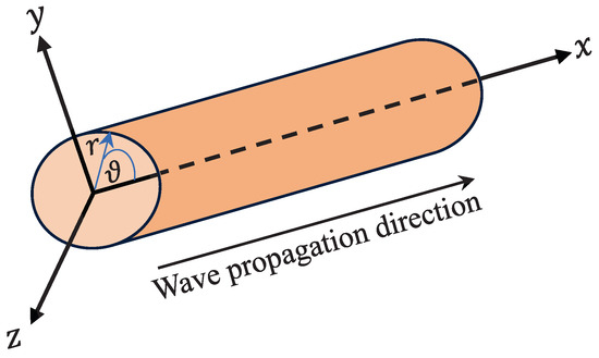
Figure 1.
Schematic of a piezoelectric-magnetic circular rod.
- The deformation of the rod occurs in axial symmetry; this means that the circumferential displacement and .
- The following relationship between the longitudinal and radial displacements is valid [40]:where is Poisson’s ratio and , ; .
- The rod is assumed to be thin; therefore, the problem is considered one-dimensional. Accordingly, the extended tractions on the rod’s lateral boundary must vanish (). This leads towhere and are, respectively, the stress and strain tensors; and stand for the electric displacement and magnetic induction, respectively; and are, respectively, the electric and magnetic fields.
According to the 3D elasticity theory and based on the above assumptions, the motion equations can be expressed as
where the normal stresses, electric displacement , and magnetic induction of the transversely isotropic PEM rod are defined as
where , , , , , and stand for the elastic, piezoelectric, dielectric, piezomagnetic, magnetic, and electromagnetic coefficients, respectively. Since , one has .
The non-zero strains, electric and magnetic fields are expressed as
where and are the electric and magnetic potentials, respectively. Inserting Equations (4) and (5) into Equation (3) results in the equations of motion in terms of , , and as
where and
Solving the first, third, and fourth equations of Equation (6) for u, , and and then substituting them into the second equation of Equation (6) leads to the following standard nonlinear wave equation (for more details, see Appendix A):
where and the coefficient represents the linear longitudinal wave velocity and N stands for the the dispersion coefficient, which are defined in Appendix A. Equation (8) is the nonlinear wave equation with respect to the axial displacement gradient of the PEM rod having lateral dispersion resulting from Poisson’s impact. Note that, if , there are no waves to propagate. While, if , there is no lateral dispersion for the longitudinal waves.
3. Painlevé Analysis
We endeavor to detect the integrability of Equation (8) by following the well-known ARS algorithm. So, we introduce the next definition.
Definition 1
(Painlevé integrability [29]). A nonlinear partial differential equation has a Painlevé property if its solution around a movable singular manifold is single-valued.
The integrability of Equation (8) is checked by performing the ARS algorithm, which is briefly presented in Appendix B, to have a self-contained article. We achieve the singularity analysis for Equation (8) by looking for the dependent variable Laurent series q in the non-characteristic singular manifold neighborhood of satisfying in the form
where and p is the negative integer that needs to be determined. To investigate the dominant behavior of the solution, we take into account the first term (9), i.e.,
Inserting the last expression into Equation (8) and balancing the most dominant, we find . To determine , the coefficient of the leading order term in the Laurent series (9), we insert (9) with into Equation (8) and, comparing the coefficient of , which is the leading term in the resulting equation, we obtain the leading behavior term coefficient in the form
The calculation of resonances, which are the powers of f at which free functions can occur in the Laurent series (9), is what we will be doing in the second step. The resonances r are possibly determined by plugging the next expansion
into Equation (8), and computing the coefficient of , we obtain
Hence, is an arbitrary function if , which are the required resonances. Note that resonance is the only acceptable negative resonance that always refers to the singular manifold arbitrariness .
Finally, we investigate whether there are enough free functions at these resonances without the necessity of movable critical singular manifolds. Thus, the dependent variable q is expanded as
By inserting the expression (14) into Equation (8) and computing the coefficients of different powers , we can prove that the Laurent series (9) does not have a sufficient number of arbitrary functions. This proves that the solution of Equation (8) is not free from movable critical singular manifolds. Hence, Equation (8) fails to possess the Painlevé property and this proves the next theorem.
Theorem 1.
The governing equation of the PEM circular rod does not have a Painlevé property.
4. Bifurcation Analysis
Based on Theorem 1, the non-integrability of the governing equation in a Painlevé sense motivates us to search for particular solutions to Equation (8). One of the most significant particular solutions is the traveling wave solution. The wave solution for Equation (8) is postulated:
where is the wave variable, k is the wave number, and is the wave velocity. Equation (8) is transformed into an ordinary differential equation as
where the primes indicate a derivative with respect to . Integrating the last equation twice with respect to and ignoring the constants of integration imply
where
are presented for the sake of simplicity. We rewrite Equation (17) as
System (19) is a conservative system because and a Hamiltonian because they are considered a Hamilton equation for the Hamiltonian
Due to the Hamiltonian H not depending explicitly on , which is equivalent to the time in Hamiltonian mechanics, it is itself a first integral or it is sometimes named a conserved quantity [41,42], i.e.,
where h is an arbitrary parameter. Thus, the issue of discovering a solution for Equation (8) is equivalent to finding a solution for the equation of motion of a particle in one dimension. This equivalent is beneficial in determining the interval of real solutions. A one-dimension differential form
is obtained by setting into Equation (21) and splitting the variables, where
The integration of both sides of (22) requires the determination of the range of the parameters and g. There are two different methods to find the required range. They are a complete discriminate system for the polynomial [43] and bifurcation analysis [41]. The most significant of them is bifurcation analysis because it provides a classification of solutions without finding them based on phase orbits, and also enables us to construct all possible wave propagations.
We initiate the calculation of the equilibrium points for the system (19) in order to investigate the phase portrait. These points are obtained by setting . Hence, the system (19) has two equilibrium points . The classification of them is determined by computing the Jacobian matrix eigenvalues at the equilibrium points for the system (19). These eigenvalues are , where det is the determinate of the Jacobi matrix calculated at the equilibrium point . Following [44], the equilibrium point is either saddle if or center if or . In addition, the Poincaré index for the equilibrium point is zero [44]. Thus, we have the following cases:
- (a)
- If , then points O and Q are saddle and centre, respectively. The phase portrait for this case is described in Figure 2a,b for and , respectively.
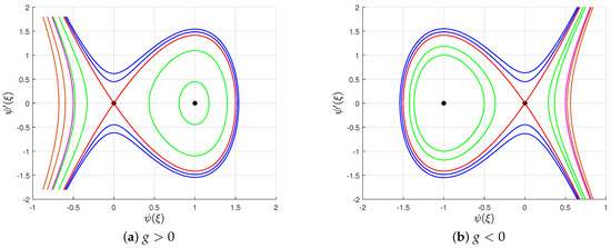 Figure 2. Phase portrait for the Hamiltonian (19) in the phase plane () for the case . The equilibria are shown by solid black circles.
 - (b)
- If , point O is centre while Q is a saddle point. The phase portrait for this case is depicted by Figure 3a,b for and , respectively.
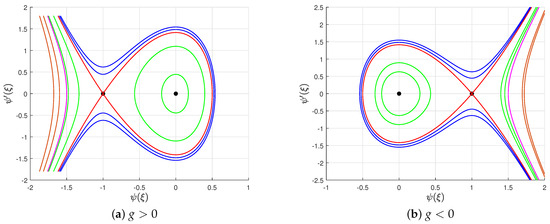 Figure 3. Phase portrait for the Hamiltonian (19) in the phase plane () for the case . The equilibria are shown by solid black circles.
The phase plane orbits are parameterized by one parameter h, i.e.,
Hence, to describe the phase plane orbits, the value of h is computed at the equilibria, i.e.,
We summarize the description of the phase plane displayed in Figure 2a in the next theorem:
Theorem 2.
For , system (19) owns the following:
- (a)
- Unbounded orbits’ family in pink, blue, and brown, respectively.
- (b)
- Two green orbits’ families . One of them is periodic around the center point Q and placed inside the homoclinic orbit in red, while the other one is unbounded and appears outside the homoclinic orbit in red.
Based on the bifurcation analysis, we introduce the next theorem.
Theorem 3.
Let us postulate that Equation (8) has a solution in the form (15). Then, it is one of the following:
- (a)
- A periodic solution if
- (b)
- A solitary solution if .
- (c)
- Otherwise, it is unbounded.
It is evident that Theorem 3 supplies the conditions of the presence of periodic solutions and solitary solutions for Equation (8). This is one of the significant benefits of the utilization of bifurcation theory.
5. Solution Construction
Based on the bifurcation constrains on the parameters and h, as outlined in Theorem 3, we can integrate both sides of Equation (22) along possible intervals of real wave propagation. In other words, for fixed values of the two parameters and distinct values of the parameters h, the solutions will be found.
- Case I:
- For , we consider the next different values of h:
- When , there are two orbit families in green for the system (19). A single orbit of this family intersects the axis at three points. Hence, the polynomial has three real roots, namely, with , i.e., it takes the form . The interval of real wave propagation is . Assuming , the integration of both sides of Equation (22) giveswhere denotes the first type of complete elliptic integrals [45]. This solution is periodic solution with period . From another side, if we consider , we assume , and consequently, the integration of both sides produces the solution
- When , the Hamilton system (19) has a homoclinic orbit in red, which connect the saddle point O to itself. Such orbits prove the existence of a solitary wave solution for Equation (8). For this case, the polynomial has one simple root while the other is double at the origin, i.e., it has the form . The intervals of real propagation are . There are two possible choices for real wave propagation. First, we assume , and consequently, the integration of both sides of Equation (22) gives the solutionwhich is the soliton solution for Equation (8).
- When , there are two unbounded orbit families for system (19) in blue and brown in addition to a single orbit in pink. All these orbits cut the axis at exactly one point. Therefore, the polynomial has one real root and two complex conjugate roots, namely, and , where refers to the complex conjugate. Hence, and the interval of real wave propagation is . We integrate Equation (22) along the interval of real wave propagation and obtainwhere .
- Case II:
- For the case , the solution of Equation (8) can be constructed according to the values of the parameter h.
- Case III:
- The two cases in which and provide the same solutions as in the two cases I and II but with different values of the roots of the polynomial .It can be demonstrated that the obtained solutions are consistent by studying their degeneracy through the transmission between phase orbits. Let us clarify the following:
- (a)
- If , the family of periodic orbits in green will be reduced to the homoclinic orbit in red, as illustrated by Figure 2a. Consequently, the periodic solution corresponding to this family will also degenerate to a solitary solution corresponding to the homoclinic orbit. Thus, we have and , and solution (26) becomeswhich is in agreement with solution (28).
- (b)
- On the other hand, when h tends to zero, the family of unbounded orbits in blue will reduce to the homoclinic orbit, and consequently, solution (29) must be transformed into solution (28). Let us outline that. When , we find and , and consequently, solution (29) becomeswhich is identical to solution (28).
6. Results and Discussion
In the current section, various numerical investigations are presented to explain the dynamic behavior of the piezoelectro-magnetic infinite circular rod under various values of wave velocity. It is assumed that the rod is made of the BaTiO-CoFeO, with a radius cm [46], Poisson’s ratio [46], and density kg/m [46]. The other mechanical and electromagnetic properties are presented in Table 1. We find that and . Assuming the wave number , wave velocity , and the radius of the rod is , we obtain , , and . Due to , the solution for Equation (8) can be constructed by utilizing case I, and moreover, the solution can be constructed based on the value of the parameter h. Let us clarify that the following applies for some possible values of the parameter h.

Table 1.
Material properties of the BaTiO-CoFeO rod [46].
- This solution is clarified by Figure 4a. Now, we study the effect of the wave velocity on the periodic solution (26) by allowing to take distinct values and the other parameters to be unchanged. It is obvious that, as the wave velocity grows, the amplitude of the periodic solution increases and the width of the solution decreases.
 Figure 4. Graphic representation of the periodic wave in PEM rod.
 - Figure 5a illustrates the 3D representation of solution (36). Figure 5b outlines the effects of the wave velocity on solution (28) for different values of while the others remain fixed on the plane . It is obvious that the curves are symmetric about the line . The amplitude of the solution increases as the value of the wave velocity grows.
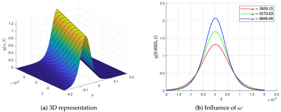 Figure 5. Graphic representation of the solitary wave in PEM rod.
We also investigate the influence of the other parameters on the obtained solutions but it is very tiny.
7. Conclusions
The current work is interested in studying some qualitative analyses of a motion equation describing the behavior of a piezoelectro-magnetic circular rod. In accordance with the three-dimensional elasticity theory, the motion equation has been established. We have shown the motion equation is non-integrable in a Painlevé sense by using the well-known ARS algorithm. As a result of its non-integrability, the search for semi-analytical solutions or numerical solutions is instructed. Therefore, we seek particular solutions, like traveling wave solutions, which can be used to explain the physical interpretations of the phenomenon. The qualitative theory of planar integrable systems has been applied to study the bifurcation of the solutions based on the material properties of the rod. The employment of the bifurcation theory encloses multiple benefits. Let us elucidate them:
- (a)
- The bifurcation theory has enabled us to prove Theorem 3, which provided the constraints on the parameters classifying the types of the solutions before constructing them.
- (b)
- Determining the intervals of real solutions, which are sometimes named the intervals of real wave propagation, is significant because it implies that there are different types of solutions that are completely different from mathematical and physical points of view. For clarification, when , we have two solutions (26) and (29) that are periodic and unbounded. The two solutions are obtained with the same conditions on the parameters , and h but with different intervals of real solutions. Hence, the interval of real solutions is significant.
We have introduced some new solutions that have been classified into double periodic solutions and solitary solutions, depending on the phase plane orbit. Taking into account the material constants of the rod, 3D representations of periodic and solitary solutions have been displayed. It is well-known that wave velocity enables us to compute the speed at which a wave travels through a medium. The magnitude of the wave velocity is the distance that the wave travels in a given time. This is of considerable importance for the propagation of information and other demonstrations of wave motion in science and engineering. Therefore, it is significant to study the influence of the wave velocity on the obtained solutions that represent the wave propagation in the rod. As the wave velocity increased while the other parameters were unchanged, it has been noticed on the plane that the amplitude and the width of the periodic solution increased and decreased, respectively. That is to say, the waves with a bigger amplitude would have a narrower width due to the dispersion feature in the nonlinear waves. Also, the amplitude of the solitary solution on the plane decreased with the growing wave velocity. The effects of the other parameters on the solutions are very tiny so can be ignored.
Author Contributions
Conceptualization, A.A.E. and M.S.; methodology, A.A.E. and M.S.; software, S.M.A., A.A.E. and M.S.; validation, S.M.A., A.A.E. and M.S.; formal analysis, S.M.A., A.A.E. and M.S.; investigation, S.M.A., A.A.E. and M.S.; resources, S.M.A., A.A.E. and M.S.; data curation, S.M.A., A.A.E. and M.S.; writing—original draft preparation, S.M.A., A.A.E. and M.S.; writing—review and editing, S.M.A., A.A.E. and M.S.; visualization, S.M.A., A.A.E. and M.S.; supervision, A.A.E. and M.S.; project administration, S.M.A., A.A.E. and M.S.; funding acquisition, S.M.A. All authors have read and agreed to the published version of the manuscript.
Funding
This work was supported by the Deanship of Scientific Research, Vice Presidency for Graduate Studies and Scientific Research, King Faisal University, Saudi Arabia (grant No. GRANT5495).
Institutional Review Board Statement
Not applicable.
Informed Consent Statement
Not applicable.
Data Availability Statement
Data are contained within the article.
Conflicts of Interest
The authors declare no conflicts of interest.
Appendix A
More clarification for deducing the nonlinear wave Equation (8) is presented in this appendix. Based on Cramer’s rule, the first, third, and fourth equations of Equation (6) can be solved to obtain , and as
where
Taking the derivative of Equation (A3) with respect to x and substituting from Equation (5) into the resulting equation leads to the following wave equation:
where
By using some mathematical manipulations, Equation (A4) can be easily converted to the following form:
where
Appendix B
In this appendix, the ARS algorithm is briefly displayed. Consider a nonlinear partial differential equation in the form
where and u are a polynomial and a complex-valued function, depending on the two variables S and t, respectively. This appendix provides a brief description of the Painlevé analysis. The Painlevé analysis is employed to determine whether the given Equation (A8) is integrable or not. The solution of Equation (A8) is assumed to be a Laurent series
where and p is a negative integer needed to be found. We follow the ARS algorithm, which can be outlined as in the subsequent steps [30]:
Step 1: Dominate behavior. The leading order term in the Laurent series (A9) is assumed to be
Inserting the expression into Equation (A8) and balancing the dominant terms, we found the value of p. The coefficient of the leading term is calculated by inserting the Laurent series with the obtained value of p into Equation (A8), and equating the coefficient of the leading term in the obtained equation, we obtain an equation determining .
Step 2: Resonances. The resonances are defined as the powers at which the arbitrary functions appear in the Laurent series. The resonance can be determined by inserting
into Equation (A8) and comparing different powers of . Notice that all the resonances are non-negative integers except the resonance , which refers to the arbitrariness of . Additionally, the resonance indicates that the coefficient of the leading term is arbitrary. If all the values of resonances are non-negative except , we go to the next step.
Step 3: Compatibility conditions. This step aims to check the existence of a sufficient number of arbitrary functions in the Laurent series (A9). This can be performed by inserting the expression
into Equation (A8) and testing the existence of arbitrary functions corresponding to the obtained resonances in step 2, where is the largest value of the resonances. If the compatibility conditions are satisfied then the given partial differential equation has a Painlevé property. Consequently, it is integrable in a Painlevé sense, which is sometimes called Painlevé integrable.
References
- Van Run, A.; Terrell, D.; Scholing, J. An in situ grown eutectic magnetoelectric composite material: Part 2 physical properties. J. Mater. Sci. 1974, 9, 1710–1714. [Google Scholar] [CrossRef]
- Boomgaard, J.v.d.; Van Run, A.; Van Suchtelen, J. Piezoelectric-piezomagnetic composites with magnetoelectric effect. Ferroelectrics 1976, 14, 727–728. [Google Scholar] [CrossRef]
- Wu, T.L.; Huang, J.H. Closed-form solutions for the magnetoelectric coupling coefficients in fibrous composites with piezoelectric and piezomagnetic phases. Int. J. Solids Struct. 2000, 37, 2981–3009. [Google Scholar] [CrossRef]
- Espinosa-Almeyda, Y.; Camacho-Montes, H.; Rodríguez-Ramos, R.; Guinovart-Díaz, R.; López-Realpozo, J.; Bravo-Castillero, J.; Sabina, F. Influence of imperfect interface and fiber distribution on the antiplane effective magneto-electro-elastic properties for fiber reinforced composites. Int. J. Solids Struct. 2017, 112, 155–168. [Google Scholar] [CrossRef]
- Sobhy, M. Magneto-electro-thermal bending of FG-graphene reinforced polymer doubly-curved shallow shells with piezoelectromagnetic faces. Compos. Struct. 2018, 203, 844–860. [Google Scholar] [CrossRef]
- Haghgoo, M.; Hassanzadeh-Aghdam, M.K.; Ansari, R. Effect of piezoelectric interphase on the effective magneto-electro-elastic properties of three-phase smart composites: A micromechanical study. Mech. Adv. Mater. Struct. 2019, 26, 1935–1950. [Google Scholar] [CrossRef]
- Hong, J.; Wang, S.; Qiu, X.; Zhang, G. Bending and Wave Propagation Analysis of Magneto-Electro-Elastic Functionally Graded Porous Microbeams. Crystals 2022, 12, 732. [Google Scholar] [CrossRef]
- Chaki, M.S.; Bravo-Castillero, J. A mathematical analysis of anti-plane surface wave in a magneto-electro-elastic layered structure with non-perfect and locally perturbed interface. Eur. J.-Mech.-A/Solids 2023, 97, 104820. [Google Scholar] [CrossRef]
- Li, L.; Lan, M.; Wei, P.; Zhang, Q. Classifications of surface waves in magneto-electro-elastic materials. Results Phys. 2023, 51, 106622. [Google Scholar] [CrossRef]
- Del Toro, R.; De Bellis, M.L.; Bacigalupo, A. High frequency multi-field continualization scheme for layered magneto-electro-elastic materials. Int. J. Solids Struct. 2023, 282, 112431. [Google Scholar] [CrossRef]
- Kuo, H.Y.; Yang, L.H.; Huang, P.C.; Pan, E. Wave characteristics in magneto-electro-elastic laminated composites with different layering directions. Acta Mech. 2023, 234, 4467–4485. [Google Scholar] [CrossRef]
- Chaki, M.S.; Bravo-Castillero, J. Dynamic asymptotic homogenization for wave propagation in magneto-electro-elastic laminated composite periodic structure. Compos. Struct. 2023, 322, 117410. [Google Scholar] [CrossRef]
- Sobhy, M.; Al Mukahal, F. Analysis of electromagnetic effects on vibration of functionally graded GPLs reinforced piezoelectromagnetic plates on an elastic substrate. Crystals 2022, 12, 487. [Google Scholar] [CrossRef]
- Sobhy, M.; Al Mukahal, F. Wave dispersion analysis of functionally graded GPLs-reinforced sandwich piezoelectromagnetic plates with a honeycomb core. Mathematics 2022, 10, 3207. [Google Scholar] [CrossRef]
- Zou, Z.; Guo, R. The Riemann–Hilbert approach for the higher-order Gerdjikov–Ivanov equation, soliton interactions and position shift. Commun. Nonlinear Sci. Numer. Simul. 2023, 124, 107316. [Google Scholar] [CrossRef]
- Shen, S.; Yang, Z.; Li, X.; Zhang, S. Periodic propagation of complex-valued hyperbolic-cosine-Gaussian solitons and breathers with complicated light field structure in strongly nonlocal nonlinear media. Commun. Nonlinear Sci. Numer. Simul. 2021, 103, 106005. [Google Scholar] [CrossRef]
- Li, X.L.; Guo, R. Interactions of Localized Wave Structures on Periodic Backgrounds for the Coupled Lakshmanan–Porsezian–Daniel Equations in Birefringent Optical Fibers. Ann. Phys. 2023, 535, 2200472. [Google Scholar] [CrossRef]
- Song, L.M.; Yang, Z.J.; Li, X.L.; Zhang, S.M. Coherent superposition propagation of Laguerre–Gaussian and Hermite–Gaussian solitons. Appl. Math. Lett. 2020, 102, 106114. [Google Scholar] [CrossRef]
- Jadaun, V.; Kumar, S. Lie symmetry analysis and invariant solutions of (3 + 1)-dimensional Calogero–Bogoyavlenskii–Schiff equation. Nonlinear Dyn. 2018, 93, 349–360. [Google Scholar] [CrossRef]
- Tu, J.M.; Tian, S.F.; Xu, M.J.; Zhang, T.T. On Lie symmetries, optimal systems and explicit solutions to the Kudryashov–Sinelshchikov equation. Appl. Math. Comput. 2016, 275, 345–352. [Google Scholar] [CrossRef]
- Taghizadeh, N.; Mirzazadeh, M.; Farahrooz, F. Exact solutions of the nonlinear Schrödinger equation by the first integral method. J. Math. Anal. Appl. 2011, 374, 549–553. [Google Scholar] [CrossRef]
- Elbrolosy, M.; Elmandouh, A. Bifurcation and new traveling wave solutions for (2 + 1)-dimensional nonlinear Nizhnik–Novikov–Veselov dynamical equation. Eur. Phys. J. Plus 2020, 135, 533. [Google Scholar] [CrossRef]
- Elmandouh, A.A.; Ibrahim, A.G. Bifurcation and travelling wave solutions for a (2 + 1)-dimensional KdV equation. J. Taibah Univ. Sci. 2020, 14, 139–147. [Google Scholar] [CrossRef]
- Elbrolosy, M.; Elmandouh, A. Dynamical behaviour of nondissipative double dispersive microstrain wave in the microstructured solids. Eur. Phys. J. Plus 2021, 136, 1–20. [Google Scholar] [CrossRef]
- Elmandouh, A.A.; Elbrolosy, M.E. New traveling wave solutions for Gilson–Pickering equation in plasma via bifurcation analysis and direct method. Math. Methods Appl. Sci. 2022. [Google Scholar] [CrossRef]
- Elmandouh, A.A.; Elbrolosy, M.E. Integrability, variational principal, bifurcation and new wave solutions for Ivancevic option pricing model. J. Math. 2022, 2, 3. [Google Scholar]
- Manukure, S.; Chowdhury, A.; Zhou, Y. Complexiton solutions to the asymmetric Nizhnik–Novikov–Veselov equation. Int. J. Mod. Phys. B 2019, 33, 1950098. [Google Scholar] [CrossRef]
- El-Dessoky, M.M.; Elmandouh, A.A. Qualitative analysis and wave propagation for Konopelchenko-Dubrovsky equation. Alex. Eng. J. 2023, 67, 525–535. [Google Scholar] [CrossRef]
- Weiss, J.; Tabor, M.; Carnevale, G. The Painlevé property for partial differential equations. J. Math. Phys. 1983, 24, 522–526. [Google Scholar] [CrossRef]
- Ablowitz, M.J.; Ramani, A.; Segur, H. A connection between nonlinear evolution equations and ordinary differential equations of P-type. II. J. Math. Phys. 1980, 21, 1006–1015. [Google Scholar] [CrossRef]
- Conte, R. Invariant Painlevé analysis of partial differential equations. Phys. Lett. A 1989, 140, 383–390. [Google Scholar] [CrossRef]
- Conte, R.; Fordy, A.P.; Pickering, A. A perturbative Painlevé approach to nonlinear differential equations. Phys. Nonlinear Phenom. 1993, 69, 33–58. [Google Scholar] [CrossRef]
- Estévez, P.; Conde, E.; Gordoa, P.R. Unified approach to Miura, Bäcklund and Darboux transformations for nonlinear partial differential equations. J. Nonlinear Math. Phys. 1998, 5, 82–114. [Google Scholar] [CrossRef]
- Jimbo, M.; Kruskal, M.; Miwa, T. Painlevé test for the self-dual Yang-Mills equation. Phys. Lett. A 1982, 92, 59–60. [Google Scholar] [CrossRef]
- Lou, S. Searching for higher dimensional integrable models from lower ones via Painlevé analysis. Phys. Rev. Lett. 1998, 80, 5027. [Google Scholar] [CrossRef]
- Hereman, W.; Göktaş, Ü.; Colagrosso, M.D.; Miller, A.J. Algorithmic integrability tests for nonlinear differential and lattice equations. Comput. Phys. Commun. 1998, 115, 428–446. [Google Scholar] [CrossRef][Green Version]
- Xu, G.; Li, Z. Symbolic computation of the Painlevé test for nonlinear partial differential equations using Maple. Comput. Phys. Commun. 2004, 161, 65–75. [Google Scholar] [CrossRef]
- Karasu, A. Painlevé classification of coupled Korteweg–de Vries systems. J. Math. Phys. 1997, 38, 3616–3622. [Google Scholar] [CrossRef]
- Sakovich, S.Y.; Tsuchida, T. Symmetrically coupled higher-order nonlinear Schrödinger equations: Singularity analysis and integrability. J. Phys. Math. Gen. 2000, 33, 7217. [Google Scholar] [CrossRef]
- Liu, Z.F.; Zhang, S.Y. Solitary waves in finite deformation elastic circular rod. Appl. Math. Mech. 2006, 27, 1255–1260. [Google Scholar] [CrossRef]
- Saha, A.; Banerjee, S. Dynamical Systems and Nonlinear Waves in Plasmas; CRC Press: Boca Raton, FL, USA, 2021. [Google Scholar]
- Goldstein, H.; Poole, C.P.; Safko, J.L. Classical Mechanics, 3rd ed.; Addison Wesley: Boston, MA, USA, 2000. [Google Scholar]
- Liang, S.; Zhang, J. A complete discrimination system for polynomials with complex coefficients and its automatic generation. Sci. China Ser. Technol. Sci. 1999, 42, 113–128. [Google Scholar] [CrossRef]
- Nemytskii, V.V.; Stepanov, V. Qualitative Theory of Differential Equations; Princeton University Press: Boston, MA, USA, 1960. [Google Scholar]
- Byrd, P.F.; Friedman, M.D. Handbook of Elliptic Integrals for Engineers and Scientists, 2nd ed.; Die Grundlehren der mathematischen Wissenschaften, Band 67; Springer-Verlag: New York, NY, USA; Heidelberg, Germany, 1971; p. xvi+358. [Google Scholar]
- Xue, C.; Pan, E.; Zhang, S. Solitary waves in a magneto-electro-elastic circular rod. Smart Mater. Struct. 2011, 20, 105010. [Google Scholar] [CrossRef]


Disclaimer/Publisher’s Note: The statements, opinions and data contained in all publications are solely those of the individual author(s) and contributor(s) and not of MDPI and/or the editor(s). MDPI and/or the editor(s) disclaim responsibility for any injury to people or property resulting from any ideas, methods, instructions or products referred to in the content. |
© 2024 by the authors. Licensee MDPI, Basel, Switzerland. This article is an open access article distributed under the terms and conditions of the Creative Commons Attribution (CC BY) license (https://creativecommons.org/licenses/by/4.0/).