SIR Epidemic Model with General Nonlinear Incidence Rate and Lévy Jumps

Abstract

This article proposes a stochastic SIR model with general nonlinear incidence and Lévy jumps, which is used to describe diseases spreading in human populations. The model takes into account the randomness and sublinearity of diseases and can more accurately describe the disease transmission process. Firstly, we prove that this stochastic SIR model has a unique global positive solution. Then, sufficient conditions for the extinction of the disease are given. We also discuss the case that the disease persists in the model. In addition, we study the asymptotic behavior of the solution of the stochastic SIR model relative to the equilibrium points of the deterministic SIR model. These results allow us to understand the trends and dynamic changes of diseases in human populations, providing theoretical support for developing more scientific and effective disease control strategies and prevention measures. Finally, we give some examples and numerical simulations to demonstrate the effectiveness and feasibility of the theoretical results.

1. Introduction and Main Results

1.1. Introduction on the Background

Infectious diseases have long been a significant challenge throughout human history, ranging from ancient plagues and the Black Death to modern-day pandemics such as influenza, AIDS, and, in recent years, the novel coronavirus. The outbreak of infectious diseases poses significant threats to human health and has profound impacts on society, the economy, and politics. Therefore, the research of infectious diseases has consistently remained a critical global agenda.

Researchers have developed a diverse array of mathematical models to gain a deeper understanding of the transmission mechanisms of infectious diseases, anticipate their developmental trends, and evaluate the effectiveness of various prevention and control strategies. Among these, differential equation-based models for infectious diseases, including the SIR model and SEIR model, have been widely used and continuously evolved. In 1927, Kermack and McKendrick [1] established the classic deterministic SIR model. They divided the population into three individuals:

(S)

Susceptible individuals—These individuals are not immune to the disease and, therefore, vulnerable to infection.

(I)

Infected individuals—These individuals are currently infected with the disease and can spread it to other susceptible individuals.

(R)

Removed individuals—These individuals have been infected with the disease, have recovered from it, and are now immune to further infection.

Let $S\left(t\right)$, $I\left(t\right)$, and $R\left(t\right)$ denote the number of susceptible individuals, infected individuals, and removed individuals, respectively, at time t. Then the classical deterministic SIR model in [2] is formulated by the following ordinary differential equations (ODEs)

$$\left\{\begin{array}{cc}\hfill \mathrm{d}S\left(t\right)=& [\alpha -\beta S\left(t\right)I\left(t\right)-{\mu }_{1}S\left(t\right)]\mathrm{d}t,\hfill \\ \hfill \mathrm{d}I\left(t\right)=& [\beta S\left(t\right)I\left(t\right)-\left({\mu }_2+\rho +\gamma \right)I\left(t\right)]\mathrm{d}t,\hfill \\ \hfill \mathrm{d}R\left(t\right)=& [\gamma I\left(t\right)-{\mu }_{3}R\left(t\right)]\mathrm{d}t,\hfill \end{array}\right.$$

(1)

where $\alpha$ is the birth rate of the population per unit time, ${\mu }_i$, $i=1,2,3$ as the natural death rates of $S\left(t\right)$, $I\left(t\right)$, and $R\left(t\right)$, respectively. $\beta$ is the effective contact rate between $S\left(t\right)$ and $I\left(t\right)$, $\gamma$ represents the recovery rate of infected individuals, and $\rho$ reflects the additional disease-induced death rate of the infected individuals. These epidemiological parameters are all positive constants. In particular, with the development of infectious disease dynamics, many results about the deterministic SIR model can be found in [3,4,5,6].

The bilinear term $\beta SI$ in the system (1) is a good approximation of the incidence to study some certain infectious diseases, such as dengue fever and avian influenza, see [7,8]. However, in the spread of some sexually transmitted diseases (STDs), such as AIDS and syphilis, etc., the number of people infected by each carrier may gradually decrease as the number of infected individuals increases. This is because people take measures to protect themselves or reduce contact with infected individuals as the disease spreads, which reduces the infection rate. However, the bilinear incidence rate assumes that each carrier can infect infinitely many people, which does not agree with the reality. In addition, the mathematical expression of the sublinear incidence rate is more complex than the bilinear incidence rate, which can better fit the actual data of disease transmission and more accurately predict the future development trend of the disease.

In [9], Zhou et al. introduced the nonlinear incidence rate $\beta Sg\left(I\right)$, where the function $g\left(I\right)$ is twice continuously differentiable and satisfies:

$$\left(i\right).g\left(0\right)=0\mathrm{and}{g}^{\prime }\left(I\right)>0,\left(ii\right).0⩽{\left(\frac{I}{g\left(I\right)}\right)}^{\prime }⩽m,\forall I⩾0.$$

(2)

Significantly, the condition (i) of $g\left(I\right)$ indicates that there will be no contact infections when no infected individuals are in the population. Besides, as the number of infected individuals increases, the risk of disease transmission will also increase accordingly. The condition (ii) of $g\left(I\right)$ reflects the assumption of sublinear incidence, where people will take measures to protect themselves or reduce contact with infected individuals, thereby reducing the infection rate. In particular, the deterministic SIR model in [9] was described by the following equations

$$\left\{\begin{array}{cc}\hfill \mathrm{d}S\left(t\right)=& [\alpha -\beta S\left(t\right)g\left(I\left(t\right)\right)-{\mu }_{1}S\left(t\right)]\mathrm{d}t,\hfill \\ \hfill \mathrm{d}I\left(t\right)=& [\beta S\left(t\right)g\left(I\left(t\right)\right)-\left({\mu }_2+\rho +\gamma \right)I\left(t\right)]\mathrm{d}t,\hfill \\ \hfill \mathrm{d}R\left(t\right)=& [\gamma I\left(t\right)-{\mu }_{3}R\left(t\right)]\mathrm{d}t,\hfill \end{array}\right.$$

(3)

and they obtained that the system (3) has an invariant attracting set

$$\mathcal{D}=\left\{(S,I,R)|S⩾0,I⩾0,R⩾0,S+I+R⩽\frac{\alpha }{min\{{\mu }_1,{\mu }_2+\rho ,{\mu }_3\}}\triangleq \Lambda \right\},$$

(4)

and the basic reproduction number is ${\mathcal{R}}_0=\frac{\alpha \beta g^{\prime }\left(0\right)}{{\mu }_1({\mu }_2+\rho +\gamma )}$. If ${\mathcal{R}}_0⩽1$, there is a disease-free equilibrium $E_0=\left(\frac{\alpha }{{\mu }_1},0,0\right)$, which is globally asymptotically stable on $\mathcal{D}$. If ${\mathcal{R}}_0>1$, $E_0$ is unstable, but there exists a unique endemic equilibrium $E_{*}=(S_{*},I_{*},R_{*})$ of system (3) and it is globally asymptotically stable on $\mathcal{D}$, where $S_{*}=\frac{({\mu }_2+\rho +\gamma )I_{*}}{\beta g\left(I_{*}\right)}$, $R_{*}=\frac{\gamma }{{\mu }_3}{I}_{*}$, and $I_{*}$ is solved by the nonlinear equation $\alpha \beta g\left(I_{*}\right)=({\mu }_2+\rho +\gamma )I_{*}[\beta g\left(I_{*}\right)+{\mu }_1]$.

In real life, due to the fact that the spread of infectious diseases is affected by many random factors, the introduction of stochastic epidemic models can provide more accurate predictions of the dynamic spread of diseases. By combining epidemic models with stochastic theory, we can better understand the mechanism of disease transmission and more accurately predict its spread, providing a solid foundation for public health departments to make scientific decisions. Therefore, stochastic epidemic models have essential application value in revealing the laws of disease transmission and formulating effective prevention and control strategies. The research on stochastic epidemic models has been emerging in recent years, leading to significant advancements. Jiang et al. [10] analyzed the asymptotic behavior of the following stochastic SIR model

$$\left\{\begin{array}{cc}\hfill \mathrm{d}S\left(t\right)=& [\alpha -\beta S\left(t\right)I\left(t\right)-\mu S\left(t\right)]\mathrm{d}t+{\sigma }_{1}S\left(t\right)\mathrm{d}{W}_1\left(t\right),\hfill \\ \hfill \mathrm{d}I\left(t\right)=& [\beta S\left(t\right)I\left(t\right)-\left(\mu +\rho +\gamma \right)I\left(t\right)]\mathrm{d}t+{\sigma }_{2}I\left(t\right)\mathrm{d}{W}_2\left(t\right),\hfill \\ \hfill \mathrm{d}R\left(t\right)=& [\gamma I\left(t\right)-\mu R\left(t\right)]\mathrm{d}t+{\sigma }_{3}R\left(t\right)\mathrm{d}{W}_3\left(t\right),\hfill \end{array}\right.$$

(5)

where $W_i\left(t\right)$ are independent standard Brownian motions with intensities ${\sigma }_i⩾0$. Liu and Jiang [11] constructed a stochastic SIR model with distributed delay, building upon the deterministic model (1) and studied the disease extinction conditions of this model. El Hajji, Sayari, and Zaghdani in [12] considered the deterministic and stochastic SIR infectious disease models with nonlinear incidence rates in continuous reactors. They studied the asymptotic behavior of the solutions and established the conditions for disease persistence and extinction.

Notably, the infectious disease models studied in the mentioned works are all affected by white noise, and their solutions exhibit continuous characteristics. However, actual population systems may be subject to sudden environmental perturbations, such as earthquakes, volcanic eruptions, and tsunamis, etc. These extreme situations can interrupt the continuity of the solution, making traditional stochastic models unable to describe the system’s dynamic behavior accurately. To capture this discontinuous, researchers introduced the Lévy jump process, a stochastic process that can capture sudden, large-scale changes. This process is particularly suitable for describing population systems affected by sudden perturbations. In biology, Lévy jump process describes many biological phenomena, including animal predation behavior and population diffusion. Recently, it has also been applied to infectious disease models to describe the spread of disease better, see [13,14,15]. In [13,14], they considered stochastic SIR models with Lévy jumps and specific incidence rates. Although these models have particular applications in specific situations, they lack generality. In [15], the authors conducted in-depth research on the dynamic behavior of SVIR models with Lévy jumps.

In this paper, we suppose that massive environmental events can affect the disease transmission rate $\beta$ in model (3), and the stochastic perturbations are of Lévy noise type, that is

$$\beta \to \beta +\sigma \mathrm{d}W\left(t\right)+\mathrm{d}J\left(t\right),$$

where $W\left(t\right)$ is a standard Brownian motion on the probability space $(\Omega ,\mathcal{F},{\left\{{\mathcal{F}}_t\right\}}_{t⩾0},\mathbb{P})$ satisfying the usual condition, and $\sigma >0$ is the intensity of $W\left(t\right)$. $J\left(t\right)={\int }_0^t{\int }_{\mathbb{Y}}Q\left(a\right)\tilde{N}(\mathrm{d}a,\mathrm{d}s)$, where $\tilde{N}(\mathrm{d}a,\mathrm{d}s)=N(\mathrm{d}a,\mathrm{d}s)-v\left(\mathrm{d}a\right)\mathrm{d}s$, and N is a Poisson counting measure with characteristic measure v on the measurable subset $\mathbb{Y}$ of $[0,\infty )$ with $v\left(\mathbb{Y}\right)<\infty$.

In this sense, the corresponding stochastic version of the system (3) with Lévy jumps is obtained as follows

$$\left\{\begin{array}{cc}\hfill \mathrm{d}S\left(t\right)=& \left(\alpha -\beta S\left(t\right)g\left(I\left(t\right)\right)-{\mu }_{1}S\left(t\right)\right)\mathrm{d}t-\sigma S\left(t\right)g\left(I\left(t\right)\right)\mathrm{d}W\left(t\right)\hfill \\ \hfill & -{\int }_{\mathbb{Y}}Q\left(a\right)S(t-)g\left(I(t-)\right)\tilde{N}(\mathrm{d}t,\mathrm{d}a),\hfill \\ \hfill \mathrm{d}I\left(t\right)=& \left(\beta S\left(t\right)g\left(I\left(t\right)\right)-\left({\mu }_2+\rho +\gamma \right)I\left(t\right)\right)\mathrm{d}t+\sigma S\left(t\right)g\left(I\left(t\right)\right)\mathrm{d}W\left(t\right)\hfill \\ \hfill & +{\int }_{\mathbb{Y}}Q\left(a\right)S(t-)g\left(I(t-)\right)\tilde{N}(\mathrm{d}t,\mathrm{d}a),\hfill \\ \hfill \mathrm{d}R\left(t\right)=& (\gamma I\left(t\right)-{\mu }_{3}R\left(t\right))\mathrm{d}t,\hfill \end{array}\right.$$

(6)

where $Q:\mathbb{Y}\times \Omega \to \mathbb{R}$ represents the effect of random jumps. We assume that Q is continuous with respect to the first variable and $\mathcal{B}\left(\mathbb{Y}\right)\times {\mathcal{F}}_t$-measurable. Here, $\mathcal{B}\left(\mathbb{Y}\right)$ is a $\sigma$-algebra on $\mathbb{Y}$.

Besides, the biological system typically possesses inherent stability and adaptability, and the evolution process of living organisms is a long-lasting, harmonious coexistence with the environment. In the face of sudden environmental changes or special events, these organisms can maintain a relatively stable state through their own regulatory and adaptive mechanisms. Over time, they have also developed a series of mechanisms and strategies to respond to external environmental disturbances. Therefore, we assume that the intensity of the jumps is nonnegative and bounded, which can be seen as an expression of the self-regulatory ability of the biological system in response to external disturbances, or an expression of the evolved adaptability of living organisms when facing the jumping behavior during the spread of infectious diseases. These assumptions bring the model closer to biological reality, enhancing its practical rationality.

Assumption 1.

$0⩽Q\left(a\right)\Lambda g^{\prime }\left(0\right)⩽\zeta <1$, $\forall a\in \mathbb{Y}$.

This article considers the random effects and the impact of emergencies on the spread of infectious disease models. It introduces a general nonlinear incidence rate, making the infectious disease model more realistic and widely applicable. This improvement enables the model to simulate the spread of infectious diseases more accurately, providing a more reliable basis for formulating prevention and control strategies. In the following content, we present the main results of this SIR model (6) in Section 1.2 and give the proofs of these results in Section 2. We provide some examples and numerical simulations in Section 3. Finally, we give a meaningful conclusion of this article in Section 4 and add an Appendix A to introduce some lemmas and necessary mathematical notations at the end.

1.2. Main Results

In order to study the dynamic behavior of the population system (6), it is necessary to consider whether the solution is positive and global. In [16], it is shown that for any given initial value, if the coefficients of the stochastic differential equation with jumps satisfy the linear growth condition and local Lipschitz continuity, the stochastic differential equation has a unique global solution (that is, it does not explode in finite time). However, the coefficients of Equation (6) do not satisfy the linear growth condition, which means that the solution of this system may explode in a finite time.

The following theorem presents the region $\mathcal{D}$ is almost surely invariant for the system (6) by using the Lyapunov analysis from [17].

Theorem 1.

For any initial value $\left(S\right(0),I(0),R(0\left)\right)\in \mathcal{D}$, this model (6) has a unique positive solution $\left(S\right(t),I(t),R(t\left)\right)\in \mathcal{D}, \forall t\ge 0 a.s.$

The basic reproduction number of infectious disease models is a crucial parameter that indicates how many healthy individuals each infected individual can transmit the disease to in a completely susceptible population. This parameter plays a pivotal role in evaluating the transmission potential of infectious diseases, predicting the spread dynamics of the illness, and devising prevention and control strategies. In deterministic model (3), the value of ${\mathcal{R}}_0$ determines whether the disease in system (3) persists or die out. In the following theorem, we establish sufficient conditions for disease extinction in the model (6) and present that noise will affect disease extinction.

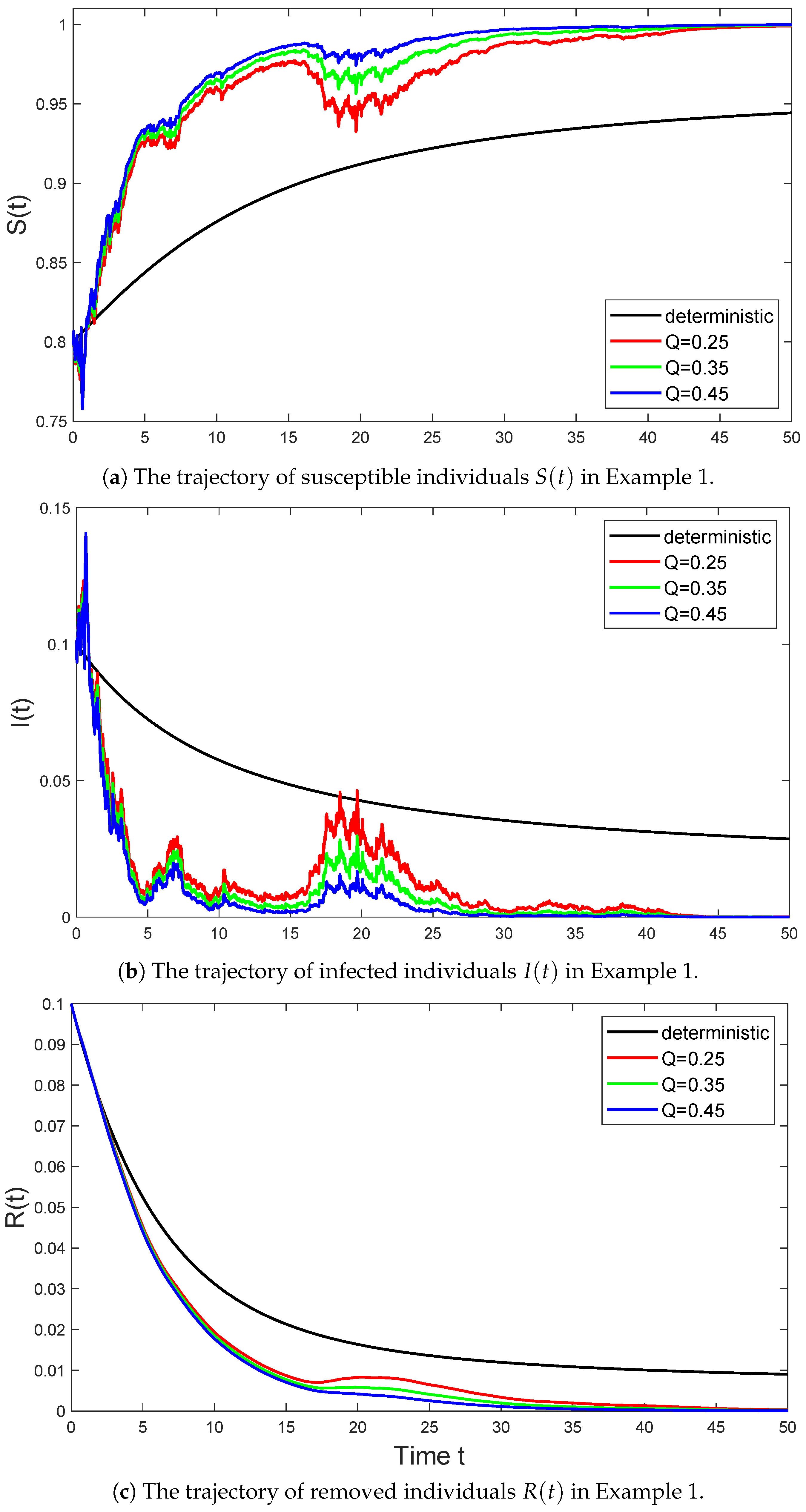
Set

$${\Theta }^2\triangleq \frac{g^2(\Lambda )}{{\Lambda }^2}\left({\sigma }^2+{\int }_{\mathbb{Y}}\frac{Q^2\left(a\right)}{{(1+\zeta )}^2}v\left(\mathrm{d}a\right)\right)\mathrm{and}{\mathcal{R}}_e\triangleq \frac{\alpha \beta g^{\prime }\left(0\right)}{{\mu }_1\left({\mu }_2+\rho +\gamma +\frac{{\alpha }^2}{2{\mu }_1^2}{\Theta }^2\right)}.$$

(7)

Theorem 2.

For any initial value $\left(S\right(0),I(0),R(0\left)\right)\in \mathcal{D}$, the solution $\left(S\right(t),I(t),R(t\left)\right)$ of system (6) satisfies

(i) 

$\underset{t\to \infty }{lim\; sup}\frac{lnI\left(t\right)}{t}⩽({\mu }_2+\rho +\gamma )\left({\mathcal{R}}_e-1\right)<0$ a.s. if ${\mathcal{R}}_e<1$ and ${\Theta }^2⩽\frac{{\mu }_1\beta g^{\prime }\left(0\right)}{\alpha }$;

(ii) 

$\underset{t\to \infty }{lim\; sup}\frac{lnI\left(t\right)}{t}⩽-({\mu }_2+\rho +\gamma )+\frac{{\beta }^2{\left(g^{\prime }\left(0\right)\right)}^2}{2{\Theta }^2}<0$ a.s. if $\frac{{\beta }^2{\left(g^{\prime }\left(0\right)\right)}^2}{2{\Theta }^2({\mu }_2+\rho +\gamma )}<1$.

Namely, the infectious disease $I\left(t\right)$ tends to zero exponentially a.s. in these two cases.

Remark 1.

(1) The expression of ${\mathcal{R}}_e$ reveals that stochastic perturbations impact the extinction of the disease in system (6). Additionally, the disease extinction condition of the model (6) is weaker than that of the model (3).

(2) The study of disease extinction can help people to utilize medical and social resources effectively. For instance, when a disease is on the verge of extinction, appropriate adjustments can be made to the allocation and utilization of medical resources to allocate more resources to treating and preventing other diseases.

In both the natural world and human society, many infectious diseases persist and evolve over time. By studying the persistence of diseases through stochastic SIR models, we can better understand the mechanisms behind disease persistence and evolution. Now, we establish sufficient conditions for the persistence of this disease in the following theorem. Firstly, the persistence in the mean of system (6) is defined as follows.

Definition 1.

System (6) is said to be persistence in the mean, if

$$\underset{t\to \infty }{lim\; inf}\frac{1}{t}{\int }_0^{t}S\left(u\right)\mathrm{d}u>0,\underset{t\to \infty }{lim\; inf}\frac{1}{t}{\int }_0^{t}I\left(u\right)\mathrm{d}u>0,\underset{t\to \infty }{lim\; inf}\frac{1}{t}{\int }_0^{t}R\left(u\right)\mathrm{d}u>0a.s.$$

(8)

Set

$${\mathcal{R}}_p\triangleq \frac{\alpha \beta }{{\mu }_1({\mu }_2+\rho +\gamma )}\frac{g(\Lambda )}{\Lambda }-\frac{{\sigma }^2{\Lambda }^2{\left(g^{\prime }\left(0\right)\right)}^2}{2({\mu }_2+\rho +\gamma )}-\frac{{\int }_{\mathbb{Y}}Q\left(a\right)\Lambda g^{\prime }\left(0\right)v\left(\mathrm{d}a\right)}{({\mu }_2+\rho +\gamma )}.$$

(9)

Theorem 3.

If ${\mathcal{R}}_p>1$, the solution $\left(S\right(t),I(t),R(t\left)\right)$ of model (6) with any initial value $\left(S\right(0),I(0),R(0\left)\right)\in \mathcal{D}$ satisfies

$$\begin{array}{cc}\hfill & \underset{t\to \infty }{lim\; inf}\frac{1}{t}{\int }_0^{t}S\left(u\right)\mathrm{d}u⩾\frac{\alpha }{\beta g(\Lambda )+{\mu }_1}>0a.s.\hfill \\ \hfill & \underset{t\to \infty }{lim\; inf}\frac{1}{t}{\int }_0^{t}I\left(u\right)\mathrm{d}u⩾\frac{{\mu }_2+\rho +\gamma }{{\mathcal{K}}_0}({\mathcal{R}}_p-1)>0a.s.\hfill \\ \hfill & \underset{t\to \infty }{lim\; inf}\frac{1}{t}{\int }_0^{t}R\left(u\right)\mathrm{d}u⩾\frac{\gamma }{{\mu }_3}\frac{{\mu }_2+\rho +\gamma }{{\mathcal{K}}_0}({\mathcal{R}}_p-1)>0a.s.\hfill \end{array}$$

where ${\mathcal{K}}_0=\beta g(\Lambda ){(\Lambda {\mu }_1({\mu }_2+\rho +\gamma ))}^{-1}$.

Remark 2.

By the condition (2) of $g\left(I\right)$, we know that ${\mathcal{R}}_p<{\mathcal{R}}_0$, this indicates that while the stochastic system (6) may rapidly approach extinction, the model (3) may continue to exist.

In 1892, Lyapunov [18] introduced the concept of stability for dynamic systems: if the trajectory of the system remains close to the equilibrium state for any initial condition, then the system is said to be Lyapunov stable under those initial conditions. This stability notion is an important theory for analyzing system stability, especially in the field of automatic control, where it is widely used in the design of dynamic systems. We use the definitions of stability introduced in [17] and demonstrate the globally stochastically asymptotically stable of system (6) on $\mathcal{D}$.

Theorem 4.

If ${\mathcal{R}}_0<1$, then the disease-free equilibrium $E_0$ is globally stochastically asymptotically stable on the region $\mathcal{D}$.

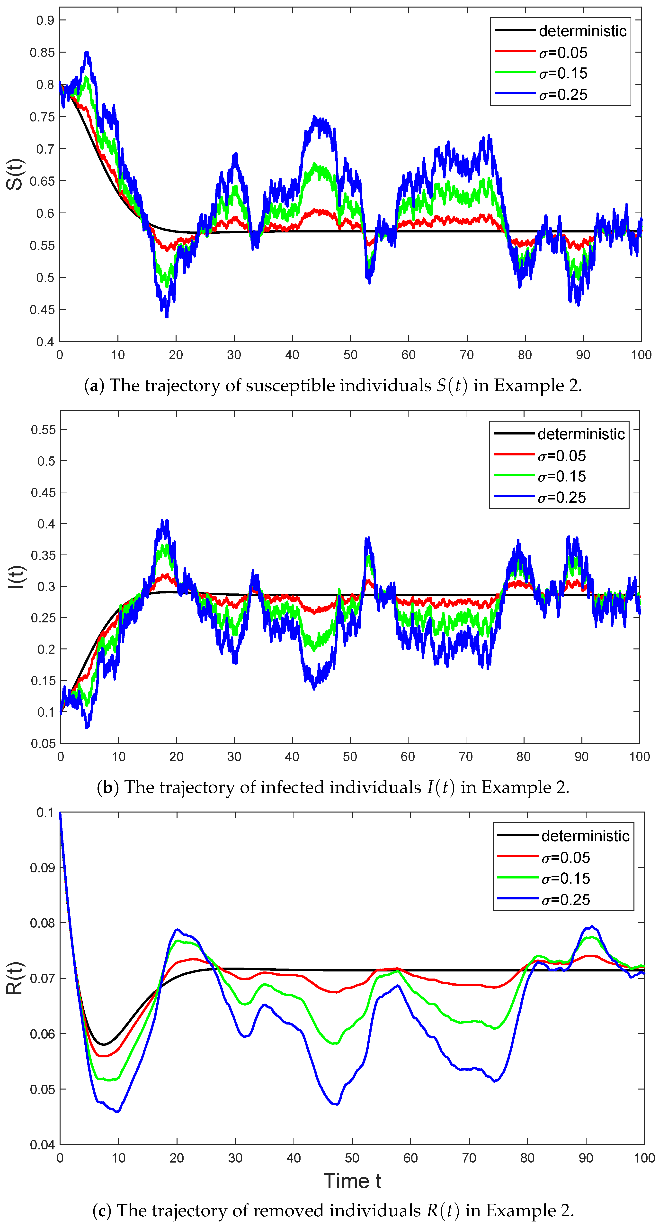
If ${\mathcal{R}}_0>1$, the deterministic SIR model (3) has an endemic equilibrium $E_{*}=(S_{*},I_{*},R_{*})$. However, $E_{*}$ is not the endemic equilibrium for stochastic system (6). Then, the dynamic of the solution $\left(S\right(t),I(t),R(t\left)\right)$ of system (6) around $E_{*}$ is discussed in the following theorem.

Theorem 5.

If ${\mathcal{R}}_0>1$ holds, then the solution of system (6) with $\left(S\right(0),I(0),R(0\left)\right)\in \mathcal{D}$ has the property

$$\underset{t\to \infty }{lim\; sup}\frac{1}{t}\mathbb{E}{\int }_0^t\left[{(S\left(u\right)-S_{*})}^2+{(I\left(u\right)-I_{*})}^2+{(R\left(u\right)-R_{*})}^2\right]\mathrm{d}u⩽\frac{K_{\sigma }}{M}.$$

where

$$\begin{array}{cc}\hfill & M=min\left\{{\mu }_1,{\mu }_2+\rho +\gamma -\frac{{\gamma }^{2}q}{2{\mu }_3},\frac{q{\mu }_3}{2}\right\},0<q<\frac{2{\mu }_3({\mu }_2+\rho +\gamma )}{{\gamma }^2},\hfill \\ \hfill & K_{\sigma }=\frac{p{I}_{*}}{2}\left({\sigma }^2{\Lambda }^2{\left(g^{\prime }\left(0\right)\right)}^2+{\int }_{\mathbb{Y}}Q\left(a\right)\Lambda g^{\prime }\left(0\right)v\left(\mathrm{d}a\right)\right).\hfill \end{array}$$

Remark 3.

Based on the above results, we can observe that as the number of random factors gradually increases, the deviation of the solution of the stochastic SIR model from the deterministic model also gradually increases. This indicates that randomness significantly impacts the spread of diseases, leading to discrepancies in epidemic trends from those predicted by deterministic models. Therefore, when formulating prevention and control strategies, it is crucial to consider the influence of random factors and adopt more flexible and effective measures to address the spread and evolution of diseases.

2. Proofs of the Main Results

2.1. Proof of Theorem 1

Proof. 

Since the coefficients of system (6) are locally Lipschitz continuous, then for any initial value $\left(S\right(0),I(0),R(0\left)\right)\in \mathcal{D}$, this system has a unique local solution for $t\in [0,{\tau }_e)$, where ${\tau }_e$ is an explosion time. In this sense, we only need to prove ${\tau }_e=\infty$. Given $k_0>0$ be sufficiently large for $S\left(0\right)>\frac{1}{k_0}$, $I\left(0\right)>\frac{1}{k_0}$ and $R\left(0\right)>\frac{1}{k_0}$. For each $k\ge k_0$, define the stopping time

$${\tau }_k=inf\left\{t\in [0,{\tau }_e):min\{S\left(t\right),I\left(t\right),R\left(t\right)\}⩽\frac{1}{k}\right\},$$

where throughout this paper we set $inf\varnothing =\infty$. Obviously, ${\tau }_k⩽{\tau }_e$ and ${\tau }_k$ is increasing as $k\to \infty$. Set ${\tau }_{\infty }={lim}_{k\to \infty }{\tau }_k$. Then, we only need to show that ${\tau }_{\infty }=\infty$. If it is false, then there exists $T>0$ and $ϵ\in (0,1)$ such that $\mathbb{P}({\tau }_{\infty }⩽T)>ϵ$. Thus there is an integer $k_1⩾k_0$ such that

$$\mathbb{P}({\tau }_k⩽T)⩾ϵ\forall k⩾k_1.$$

(10)

Define a nonnegative function V: ${\mathbb{R}}_{+}^3\to {\mathbb{R}}_{+}$ by

$$V(S,I,R)=\left(S-a_1-a_{1}ln(S/a_1)\right)+(I-1-lnI)+(R-1-lnR),$$

where $a_1$ is a positive constant to be determined later.

Applying Itô’s formula, we obtain

$$\begin{array}{cc}\hfill \mathrm{d}V=& \mathcal{L}V\mathrm{d}t+\sigma g\left(I\right)\left(a_1-S/I\right)\mathrm{d}W\left(t\right)\hfill \\ \hfill & -{\int }_{\mathbb{Y}}\left[a_{1}ln(1-Q\left(a\right)g\left(I\right))+ln\left(1+Q\left(a\right)Sg\left(I\right)/I\right)\right]\tilde{N}(\mathrm{d}t,\mathrm{d}a),\hfill \end{array}$$

(11)

where

$$\begin{array}{cc}\hfill \mathcal{L}V=& \left(1-\frac{a_1}{S}\right)\left(\alpha -\beta Sg\left(I\right)-{\mu }_{1}S\right)+\left(1-\frac{1}{I}\right)\left(\beta Sg\left(I\right)-\left({\mu }_2+\rho +\gamma \right)I\right)\hfill \\ \hfill & +\left(1-\frac{1}{R}\right)(\gamma I-{\mu }_{3}R)+\frac{a_1}{2}{\sigma }^2{g}^2\left(I\right)+\frac{1}{2I^2}{\sigma }^2{S}^2{g}^2\left(I\right)\hfill \\ \hfill & -a_1{\int }_{\mathbb{Y}}[Q\left(a\right)g\left(I\right)+ln(1-Q\left(a\right)g\left(I\right))]v\left(\mathrm{d}a\right)\hfill \\ \hfill & +{\int }_{\mathbb{Y}}\left[Q\left(a\right)Sg\left(I\right)/I-ln\left(1+Q\left(a\right)g\left(I\right)/I\right)\right]v\left(\mathrm{d}a\right).\hfill \end{array}$$

By the condition (2) of $g\left(I\right)$, we can have ${\left(g\left(I\right)/I\right)}^{\prime }=(I{g}^{\prime }\left(I\right)-g\left(I\right))/I^2⩽0$, which means that

$$\frac{g(\Lambda )}{\Lambda }⩽\frac{g\left(I\right)}{I}⩽\underset{I\to 0+}{lim}\frac{g\left(I\right)}{I}=g^{\prime }\left(0\right)\mathrm{for}\mathrm{any}I⩾0.$$

(12)

Thus, we have

$$\begin{array}{cc}\hfill \mathcal{L}V⩽& \alpha +a_1{\mu }_1+{\mu }_2+\rho +\gamma +{\mu }_3+[a_1\beta g^{\prime }\left(0\right)-({\mu }_2+\rho )]I\hfill \\ \hfill & +\frac{a_1}{2}{\sigma }^2{g}^2(\Lambda )+\frac{1}{2}{\sigma }^2{\Lambda }^2{\left(g^{\prime }\left(0\right)\right)}^2\hfill \\ \hfill & -a_1{\int }_{\mathbb{Y}}[Q\left(a\right)g\left(I\right)+ln(1-Q\left(a\right)g\left(I\right))]v\left(\mathrm{d}a\right)\hfill \\ \hfill & +{\int }_{\mathbb{Y}}\left[Q\left(a\right)Sg\left(I\right)/I-ln\left(1+Q\left(a\right)g\left(I\right)/I\right)\right]v\left(\mathrm{d}a\right).\hfill \end{array}$$

Choose $a_1=({\mu }_2+\rho )/\left(\beta g^{\prime }\left(0\right)\right)$ such that $a_1\beta g^{\prime }\left(0\right)-({\mu }_2+\rho )=0$, then

$$\begin{array}{cc}\hfill \mathcal{L}V⩽& \alpha +a_1{\mu }_1+{\mu }_2+\rho +\gamma +{\mu }_3+\frac{a_1}{2}{\sigma }^2{g}^2(\Lambda )+\frac{1}{2}{\sigma }^2{\Lambda }^2{\left(g^{\prime }\left(0\right)\right)}^2\hfill \\ \hfill & -a_1{\int }_{\mathbb{Y}}[Q\left(a\right)g\left(I\right)+ln(1-Q\left(a\right)g\left(I\right))]v\left(\mathrm{d}a\right)\hfill \\ \hfill & +{\int }_{\mathbb{Y}}\left[Q\left(a\right)Sg\left(I\right)/I-ln\left(1+Q\left(a\right)g\left(I\right)/I\right)\right]v\left(\mathrm{d}a\right).\hfill \end{array}$$

By the Assumption 1 and (12), we can obtain that

$$\begin{array}{cc}\hfill & 1-Q\left(a\right)g\left(I\right)⩾1-Q\left(a\right)I{g}^{\prime }\left(0\right)⩾1-Q\left(a\right)\Lambda g^{\prime }\left(0\right)>0,\hfill \\ \hfill & 1-Q\left(a\right)Sg\left(I\right)/I⩾1-Q\left(a\right)S{g}^{\prime }\left(0\right)⩾1-Q\left(a\right)\Lambda g^{\prime }\left(0\right)>0.\hfill \end{array}$$

In addition, by Taylor–Lagrange’s formula,

$$\begin{array}{cc}\hfill & -Q\left(a\right)g\left(I\right)-ln(1-Q\left(a\right)g\left(I\right))⩽\frac{1}{2{(1-\zeta )}^2},\hfill \end{array}$$

(13)

$$\begin{array}{cc}\hfill & Q\left(a\right)S\frac{g\left(I\right)}{I}-ln\left(1+Q\left(a\right)S\frac{g\left(I\right)}{I}\right)⩽\frac{1}{2{(1-\zeta )}^2}.\hfill \end{array}$$

(14)

Thus,

$$\begin{array}{cc}\hfill \mathcal{L}V⩽& \alpha +a_1{\mu }_1+{\mu }_2+\rho +\gamma +{\mu }_3+\frac{a_1}{2}{\sigma }^2{g}^2(\Lambda )+\frac{1}{2}{\sigma }^2{\Lambda }^2{\left(g^{\prime }\left(0\right)\right)}^2+\frac{(a_1+1)v\left(\mathbb{Y}\right)}{2{(1-\zeta )}^2}\hfill \\ \hfill \triangleq & K.\hfill \end{array}$$

(15)

Combining (11) and (15), we can have

$$\begin{array}{cc}\hfill \mathrm{d}V⩽& K\mathrm{d}t+\sigma g\left(I\right)\left(a_1-S/I\right)\mathrm{d}W\left(t\right)\hfill \\ \hfill & -{\int }_{\mathbb{Y}}\left[a_{1}ln(1-Q\left(a\right)g\left(I\right))+ln\left(1+Q\left(a\right)Sg\left(I\right)/I\right)\right]\tilde{N}(\mathrm{d}t,\mathrm{d}a).\hfill \end{array}$$

(16)

Integrating both sides of (16) from 0 to ${\tau }_k\wedge T$ and taking expectation, we obtain

$$\mathbb{E}\left[V(S({\tau }_k\wedge T),I({\tau }_k\wedge T),R({\tau }_k\wedge T))\right]⩽V(S\left(0\right),I\left(0\right),R\left(0\right))+KT.$$

(17)

Set ${\Omega }_k=\{{\tau }_k⩽T\}$ for $k⩾k_1$. By (10), we have $P\left({\Omega }_k\right)⩾ϵ$. Note, that $\forall \omega \in {\Omega }_k$, we have either $S\left({\tau }_k,\omega \right)$, or $I\left({\tau }_k,\omega \right)$, or $R\left({\tau }_k,\omega \right)$ equals $\frac{1}{k}$, and therefore,

$$V(S\left({\tau }_k,\omega \right),I\left({\tau }_k,\omega \right),R\left({\tau }_k,\omega \right))⩾1/k-1+lnk.$$

It then follows from (17)

$$V(S\left(0\right),I\left(0\right),R\left(0\right))+KT⩾\mathbb{E}\left[I_{{\Omega }_k}V(S\left({\tau }_k\right),I\left({\tau }_k\right),R\left({\tau }_k\right))\right]⩾ϵ\left[1/k-1+lnk\right],$$

where $I_{{\Omega }_k}$ is the indicator function of ${\Omega }_k$. Letting $k\to \infty$, we have

$$KT+V\left(S\left(0\right),I\left(0\right)\right)=\infty ,$$

which is a contradiction. Hence, we must have ${\tau }_{\infty }=\infty$, which implies $S\left(t\right)$, $I\left(t\right)$, and $R\left(t\right)$ will not become extinct in a finite time with probability one. □

2.2. Proof of Theorem 2

Proof. 

According to Equation (6), we have

$$\mathrm{d}(S\left(t\right)+I\left(t\right))=\left(\alpha -{\mu }_{1}S\left(t\right)-({\mu }_2+\rho +\gamma )I\left(t\right)\right)\mathrm{d}t.$$

(18)

Integrating both sides of (18) from 0 to t and dividing by t, we have

$$\frac{1}{t}{\int }_0^{t}S\left(u\right)\mathrm{d}u=\frac{\alpha }{{\mu }_1}-\frac{{\mu }_2+\rho +\gamma }{{\mu }_1}\frac{1}{t}{\int }_0^{t}I\left(u\right)\mathrm{d}u+\psi \left(t\right),$$

(19)

where

$$\psi \left(t\right)=-t^{-1}{\mu }_1^{-1}\left(S\left(t\right)-S\left(0\right)+I\left(t\right)-I\left(0\right)\right).$$

Since $\left(S\right(0),I(0\left)\right)\in \mathcal{D}$, then $\left(S\right(t),I(t\left)\right)\in \mathcal{D}$ by Theorem 1, and we have

$$\underset{t\to \infty }{lim}\psi \left(t\right)=0a.s.$$

(20)

Applying Itô’s formula to $lnI\left(t\right)$, yields

$$\begin{array}{cc}\hfill \mathrm{d}lnI\left(t\right)=& \left\{\beta S\left(t\right)\frac{g\left(I\right(t\left)\right)}{I\left(t\right)}-({\mu }_2+\rho +\gamma )-\frac{1}{2}{\sigma }^2{S}^2\left(t\right)\frac{g^2\left(I\left(t\right)\right)}{I^2\left(t\right)}\right.\hfill \\ \hfill & +\left.{\int }_{\mathbb{Y}}\left[ln\left(1+Q\left(a\right)S\left(t\right)\frac{g\left(I\right(t\left)\right)}{I\left(t\right)}\right)-Q\left(a\right)S\left(t\right)\frac{g\left(I\right(t\left)\right)}{I\left(t\right)}\right]v\left(\mathrm{d}a\right)\right\}\mathrm{d}t\hfill \\ \hfill & +\sigma S\left(t\right)\frac{g\left(I\right(t\left)\right)}{I\left(t\right)}\mathrm{d}W\left(t\right)+{\int }_{\mathbb{Y}}ln\left(1+Q\left(a\right)S\left(t\right)\frac{g\left(I\right(t\left)\right)}{I\left(t\right)}\right)\tilde{N}(\mathrm{d}t,\mathrm{d}a).\hfill \end{array}$$

(21)

Similar to (14), by (12) and Taylor–Lagrange’s formula, we also have

$$\begin{array}{cc}\hfill \mathrm{d}lnI\left(t\right)⩽& \left[\beta S\left(t\right)g^{\prime }\left(0\right)-({\mu }_2+\rho +\gamma )-\frac{1}{2}{\sigma }^2{S}^2\left(t\right)\frac{g^2(\Lambda )}{{\Lambda }^2}\right.\hfill \\ \hfill & \left.-\frac{g^2(\Lambda )}{{\Lambda }^2}{S}^2\left(t\right){\int }_{\mathbb{Y}}\frac{Q^2\left(a\right)}{2{(1+\zeta )}^2}v\left(\mathrm{d}a\right)\right]\mathrm{d}t+\sigma S\left(t\right)\frac{g\left(I\right(t\left)\right)}{I\left(t\right)}\mathrm{d}W\left(t\right)\hfill \\ \hfill & +{\int }_{\mathbb{Y}}ln\left(1+Q\left(a\right)S\left(t\right)\frac{g\left(I\right(t\left)\right)}{I\left(t\right)}\right)\tilde{N}(\mathrm{d}t,\mathrm{d}a).\hfill \end{array}$$

(22)

Integrating from 0 to t and dividing by t on both sides of (22), and by the expression of ${\Theta }^2$ in (7) and the Cauchy-Schwarz inequality, we obtain that

$$\begin{array}{cc}\hfill \frac{lnI\left(t\right)}{t}⩽& \frac{lnI\left(0\right)}{t}+\beta g^{\prime }\left(0\right)\frac{1}{t}{\int }_0^{t}S\left(u\right)\mathrm{d}u-({\mu }_2+\rho +\gamma )\hfill \\ \hfill & -\frac{1}{2}\frac{g^2(\Lambda )}{{\Lambda }^2}\left({\sigma }^2+{\int }_{\mathbb{Y}}\frac{Q^2\left(a\right)}{{(1+\zeta )}^2}v\left(\mathrm{d}a\right)\right)\frac{1}{t}{\int }_0^t{S}^2\left(u\right)\mathrm{d}u\hfill \\ \hfill & +\frac{1}{t}{\int }_0^t\sigma S\frac{g\left(I\right)}{I}\mathrm{d}W\left(u\right)+\frac{1}{t}{\int }_0^t{\int }_{\mathbb{Y}}ln\left(1+Q\left(a\right)S\frac{g\left(I\right)}{I}\right)\tilde{N}(\mathrm{d}u,\mathrm{d}a)\hfill \\ \hfill ⩽& \frac{lnI\left(0\right)}{t}+\beta g^{\prime }\left(0\right)\frac{1}{t}{\int }_0^{t}S\left(u\right)\mathrm{d}u-\frac{1}{2}{\Theta }^2{\left(\frac{1}{t}{\int }_0^{t}S\left(u\right)\mathrm{d}u\right)}^2-({\mu }_2+\rho +\gamma )\hfill \\ \hfill & +\frac{1}{t}{\int }_0^t\sigma S\frac{g\left(I\right)}{I}\mathrm{d}W\left(u\right)+\frac{1}{t}{\int }_0^t{\int }_{\mathbb{Y}}ln\left(1+Q\left(a\right)S\left(u\right)\frac{g\left(I\right(u\left)\right)}{I\left(u\right)}\right)\tilde{N}(\mathrm{d}u,\mathrm{d}a).\hfill \end{array}$$

(23)

Substituting (19) into (23), we obtain

$$\begin{array}{cc}\hfill \frac{lnI\left(t\right)}{t}⩽& \frac{lnI\left(0\right)}{t}+\beta g^{\prime }\left(0\right)\left(\frac{\alpha }{{\mu }_1}-\frac{{\mu }_2+\rho +\gamma }{{\mu }_1}\frac{1}{t}{\int }_0^{t}I\left(u\right)\mathrm{d}u+\psi \left(t\right)\right)-({\mu }_2+\rho +\gamma )\hfill \\ \hfill & -\frac{{\Theta }^2}{2}{\left(\frac{\alpha }{{\mu }_1}-\frac{{\mu }_2+\rho +\gamma }{{\mu }_1}\frac{1}{t}{\int }_0^{t}I\left(u\right)\mathrm{d}u+\psi \left(t\right)\right)}^2+\frac{\sigma }{t}{\int }_0^{t}S\frac{g\left(I\right)}{I}\mathrm{d}W\left(u\right)\hfill \\ \hfill & +\frac{1}{t}{\int }_0^t{\int }_{\mathbb{Y}}ln\left(1+Q\left(a\right)S\left(u\right)\frac{g\left(I\right(u\left)\right)}{I\left(u\right)}\right)\tilde{N}(\mathrm{d}u,\mathrm{d}a)\hfill \\ \hfill =& \beta g^{\prime }\left(0\right)\frac{\alpha }{{\mu }_1}-\frac{{\Theta }^2}{2}\frac{{\alpha }^2}{{\mu }_1^2}-({\mu }_2+\rho +\gamma )-\frac{{\Theta }^2{({\mu }_2+\rho +\gamma )}^2}{2{\mu }_1^2}{\left(\frac{1}{t}{\int }_0^{t}I\left(u\right)\mathrm{d}u\right)}^2\hfill \\ \hfill & -\frac{{\mu }_2+\rho +\gamma }{{\mu }_1}\left(\beta g^{\prime }\left(0\right)-\frac{{\Theta }^2\alpha }{{\mu }_1}\right)\frac{1}{t}{\int }_0^{t}I\left(u\right)\mathrm{d}u+\phi \left(t\right),\hfill \end{array}$$

(24)

where

$$\begin{array}{cc}\hfill \phi \left(t\right)=& \frac{lnI\left(0\right)}{t}+\beta g^{\prime }\left(0\right)\psi \left(t\right)-\frac{1}{2}{\Theta }^2{\psi }^2\left(t\right)-{\Theta }^2\frac{\alpha }{{\mu }_1}\psi \left(t\right)\hfill \\ \hfill & +\frac{{\Theta }^2({\mu }_2+\rho +\gamma )}{{\mu }_1}\psi \left(t\right)\frac{1}{t}{\int }_0^{t}I\left(u\right)\mathrm{d}u+\frac{1}{t}{\int }_0^t\sigma S\left(u\right)\frac{g\left(I\right(u\left)\right)}{I\left(u\right)}\mathrm{d}W\left(u\right)\hfill \\ \hfill & +\frac{1}{t}{\int }_0^t{\int }_{\mathbb{Y}}ln\left(1+Q\left(a\right)S\left(u\right)\frac{g\left(I\right(u\left)\right)}{I\left(u\right)}\right)\tilde{N}(\mathrm{d}u,\mathrm{d}a).\hfill \end{array}$$

Moreover, by (2), (12) and Theorem 1, we have

$$\begin{array}{cc}\hfill & {\int }_0^t{\sigma }^2{S}^2\left(u\right)\frac{g^2\left(I\left(u\right)\right)}{I^2\left(u\right)}\mathrm{d}u⩽{\sigma }^2{\Lambda }^2{\left(g^{\prime }\left(0\right)\right)}^{2}t,\hfill \\ \hfill & {\int }_0^t{\int }_{\mathbb{Y}}{\left(ln\left(1+Q\left(a\right)S\left(u\right)\frac{g\left(I\right(u\left)\right)}{I\left(u\right)}\right)\right)}^{2}v\left(\mathrm{d}a\right)\mathrm{d}u⩽{(ln(1+\zeta ))}^{2}v\left(\mathbb{Y}\right)t.\hfill \end{array}$$

(25)

In view of Lemma A1 and (20), $\phi \left(t\right)$ satisfies

$$\underset{t\to \infty }{lim}\phi \left(t\right)=0.$$

(26)

By (24), if ${\mathcal{R}}_e<1$ and ${\Theta }^2⩽{\mu }_1\beta g^{\prime }\left(0\right)/\alpha$ hold, we have

$$\begin{array}{cc}\hfill \frac{lnI\left(t\right)}{t}⩽& \beta g^{\prime }\left(0\right)\frac{\alpha }{{\mu }_1}-\frac{1}{2}{\Theta }^2\frac{{\alpha }^2}{{\mu }_1^2}-({\mu }_2+\rho +\gamma )+\phi \left(t\right)\hfill \\ \hfill =& \left({\mu }_2+\rho +\gamma +{\alpha }^2{\Theta }^2/\left(2{\mu }_1^2\right)\right)({\mathcal{R}}_e-1)+\phi \left(t\right).\hfill \end{array}$$

(27)

Since $\underset{t\to \infty }{lim}\phi \left(t\right)=0$, taking the limit superior on both sides of (27), we have

$$\underset{t\to \infty }{lim\; sup}\frac{lnI\left(t\right)}{t}⩽\left({\mu }_2+\rho +\gamma +\frac{{\alpha }^2}{2{\mu }_1^2}{\Theta }^2\right)({\mathcal{R}}_e-1)<0a.s.$$

(28)

On the other hand, according to (22), we can also obtain that

$$\begin{array}{cc}\hfill \frac{lnI\left(t\right)}{t}⩽& \frac{lnI\left(0\right)}{t}+\beta g^{\prime }\left(0\right)\frac{1}{t}{\int }_0^{t}S\left(u\right)\mathrm{d}u-\frac{1}{2}{\Theta }^2{\left(\frac{1}{t}{\int }_0^{t}S\left(u\right)\mathrm{d}u\right)}^2-({\mu }_2+\rho +\gamma )\hfill \\ \hfill & +\frac{1}{t}{\int }_0^t\sigma S\frac{g\left(I\right)}{I}\mathrm{d}W\left(u\right)+\frac{1}{t}{\int }_0^t{\int }_{\mathbb{Y}}ln\left(1+Q\left(a\right)S\frac{g\left(I\right)}{I}\right)\tilde{N}(\mathrm{d}u,\mathrm{d}a)\hfill \\ \hfill =& -\frac{{\Theta }^2}{2}{\left(\frac{1}{t}{\int }_0^{t}S\left(u\right)\mathrm{d}u-\frac{\beta g^{\prime }\left(0\right)}{{\Theta }^2}\right)}^2-({\mu }_2+\rho +\gamma )+\frac{{\beta }^2{\left(g^{\prime }\left(0\right)\right)}^2}{2{\Theta }^2}+\frac{lnI\left(0\right)}{t}\hfill \\ \hfill & +\frac{\sigma }{t}{\int }_0^{t}S\frac{g\left(I\right)}{I}\mathrm{d}W\left(u\right)+\frac{1}{t}{\int }_0^t{\int }_{\mathbb{Y}}ln\left(1+Q\left(a\right)S\frac{g\left(I\right)}{I}\right)\tilde{N}(\mathrm{d}u,\mathrm{d}a)\hfill \\ \hfill ⩽& -({\mu }_2+\rho +\gamma )+\frac{{\beta }^2{\left(g^{\prime }\left(0\right)\right)}^2}{2{\Theta }^2}+\frac{lnI\left(0\right)}{t}+\frac{1}{t}{\int }_0^t\sigma S\frac{g\left(I\right)}{I}\mathrm{d}W\left(u\right)\hfill \\ \hfill & +\frac{1}{t}{\int }_0^t{\int }_{\mathbb{Y}}ln\left(1+Q\left(a\right)S\frac{g\left(I\right)}{I}\right)\tilde{N}(\mathrm{d}u,\mathrm{d}a).\hfill \end{array}$$

If $\frac{{\beta }^2{\left(g^{\prime }\left(0\right)\right)}^2}{2{\Theta }^2({\mu }_2+\rho +\gamma )}<1$ holds, using the strong law of large numbers for local martingales in Lemma A1 again, we have

$$\underset{t\to \infty }{lim\; sup}\frac{lnI\left(t\right)}{t}⩽-({\mu }_2+\rho +\gamma )+\frac{{\beta }^2{\left(g^{\prime }\left(0\right)\right)}^2}{2{\Theta }^2}<0a.s.$$

(29)

Equations (28) and (29) both imply ${lim}_{t\to \infty }I\left(t\right)=0$ a.s. Thus, the epidemic of system (6) will exponentially go to extinction with probability one under certain conditions. The decay rate of (28) is at least $({\mu }_2+\rho +\gamma +{\alpha }^2{\Theta }^2/\left(2{\mu }_1^2\right))({\mathcal{R}}_e-1)$, and the decay rate of (29) is at least $-({\mu }_2+\rho +\gamma )+\left({\beta }^2{\left(g^{\prime }\left(0\right)\right)}^2\right)/\left(2{\Theta }^2\right)$. □

2.3. Proof of Theorem 3

Proof. 

Since $I\left(t\right)\in \mathcal{D}$, according to the stochastic differential equation of $S\left(t\right)$ in (6), we can have

$$\begin{array}{cc}\hfill \mathrm{d}S\left(t\right)⩾& \left(\alpha -\beta S\left(t\right)g(\Lambda )-{\mu }_{1}S\left(t\right)\right)\mathrm{d}t-\sigma S\left(t\right)g\left(I\left(t\right)\right)\mathrm{d}W\left(t\right)\hfill \\ \hfill & -{\int }_{\mathbb{Y}}Q\left(a\right)S(t-)g\left(I(t-)\right)\tilde{N}(\mathrm{d}t,\mathrm{d}a).\hfill \end{array}$$

(30)

Integrating from 0 to t and dividing by t on both sides of (30), we obtain

$$\begin{array}{cc}\hfill (\beta g(\Lambda )+{\mu }_1)\frac{1}{t}{\int }_0^{t}S\left(u\right)\mathrm{d}u⩾& \alpha -\frac{S\left(t\right)-S\left(0\right)}{t}-\frac{1}{t}{\int }_0^t\sigma S\left(u\right)g\left(I\left(u\right)\right)\mathrm{d}W\left(u\right)\hfill \\ \hfill & -\frac{1}{t}{\int }_0^t{\int }_{\mathbb{Y}}Q\left(a\right)S(u-)g\left(I(u-)\right)\tilde{N}(\mathrm{d}u,\mathrm{d}a).\hfill \end{array}$$

Similar to (25), using the strong law of large numbers for local martingales in Lemma A1, we also have

$$\underset{t\to \infty }{lim}\left(-\frac{S\left(t\right)-S\left(0\right)}{t}-\frac{1}{t}{\int }_0^t\sigma Sg\left(I\right)\mathrm{d}W\left(u\right)-\frac{1}{t}{\int }_0^t{\int }_{\mathbb{Y}}Q\left(a\right)Sg\left(I\right)\tilde{N}(\mathrm{d}u,\mathrm{d}a)\right)=0a.s.$$

Hence,

$$\underset{t\to \infty }{lim\; inf}\frac{1}{t}{\int }_0^{t}S\left(u\right)\mathrm{d}u⩾\frac{\alpha }{\beta g(\Lambda )+{\mu }_1}a.s.$$

(31)

For infected individuals $I\left(t\right)$, since $ln\left(1+Q\left(a\right)S\frac{g\left(I\right)}{I}\right)-Q\left(a\right)S\frac{g\left(I\right)}{I}⩾-Q\left(a\right)\Lambda g^{\prime }\left(0\right)$, we can rewrite (21) as follows

$$\begin{array}{cc}\hfill \mathrm{d}lnI\left(t\right)⩾& \left[\beta \frac{g(\Lambda )}{\Lambda }S\left(t\right)-({\mu }_2+\rho +\gamma )-\frac{1}{2}{\sigma }^2{\Lambda }^2{\left(g^{\prime }\left(0\right)\right)}^2-{\int }_{\mathbb{Y}}Q\left(a\right)\Lambda g^{\prime }\left(0\right)v\left(\mathrm{d}a\right)\right]\mathrm{d}t\hfill \\ \hfill & +\sigma S\left(t\right)\frac{g\left(I\right(t\left)\right)}{I\left(t\right)}\mathrm{d}W\left(t\right)+{\int }_{\mathbb{Y}}ln\left(1+Q\left(a\right)S\left(t\right)\frac{g\left(I\right(t\left)\right)}{I\left(t\right)}\right)\tilde{N}(\mathrm{d}t,\mathrm{d}a).\hfill \end{array}$$

(32)

Integrating from 0 to t on both sides of (32), we obtain

$$\begin{array}{cc}\hfill lnI\left(t\right)⩾& lnI\left(0\right)+\beta \frac{g(\Lambda )}{\Lambda }{\int }_0^{t}S\left(u\right)\mathrm{d}u-({\mu }_2+\rho +\gamma )t-\frac{1}{2}{\sigma }^2{\Lambda }^2{\left(g^{\prime }\left(0\right)\right)}^{2}t\hfill \\ \hfill & -t{\int }_{\mathbb{Y}}Q\left(a\right)\Lambda g^{\prime }\left(0\right)v\left(\mathrm{d}a\right)+{\int }_0^t\sigma S\left(u\right)\frac{g\left(I\right(u\left)\right)}{I\left(u\right)}\mathrm{d}W\left(u\right)\hfill \\ \hfill & +{\int }_0^t{\int }_{\mathbb{Y}}ln\left(1+Q\left(a\right)S\left(u\right)\frac{g\left(I\right(u\left)\right)}{I\left(u\right)}\right)\tilde{N}(\mathrm{d}u,\mathrm{d}a),\hfill \end{array}$$

(33)

Substituting (19) into (33), and by the expression of ${\mathcal{K}}_0$ and ${\mathcal{R}}_p$, we have

$$\begin{array}{cc}\hfill lnI\left(t\right)⩾& lnI\left(0\right)+\frac{\alpha \beta }{{\mu }_1}\frac{g(\Lambda )}{\Lambda }t-({\mu }_2+\rho +\gamma )t-\frac{1}{2}{\sigma }^2{\Lambda }^2{\left(g^{\prime }\left(0\right)\right)}^{2}t\hfill \\ \hfill & -t{\int }_{\mathbb{Y}}Q\left(a\right)\Lambda g^{\prime }\left(0\right)v\left(\mathrm{d}a\right)-({\mu }_2+\rho +\gamma )\beta \frac{g(\Lambda )}{{\mu }_1\Lambda }{\int }_0^{t}I\left(u\right)\mathrm{d}u\hfill \\ \hfill & +\beta \frac{g(\Lambda )}{\Lambda }\psi \left(t\right)t+{\int }_0^t\frac{\sigma S\left(u\right)g\left(I\right(u\left)\right)}{I\left(u\right)}\mathrm{d}W\left(u\right)\hfill \\ \hfill & +{\int }_0^t{\int }_{\mathbb{Y}}ln\left(1+\frac{Q\left(a\right)S\left(u\right)g\left(I\right(u\left)\right)}{I\left(u\right)}\right)\tilde{N}(\mathrm{d}u,\mathrm{d}a)\hfill \\ \hfill =& lnI\left(0\right)+\left[({\mu }_2+\rho +\gamma )({\mathcal{R}}_p-1)\right]t-{\mathcal{K}}_0{\int }_0^{t}I\left(u\right)\mathrm{d}u+\varphi \left(t\right),\hfill \end{array}$$

(34)

where

$$\begin{array}{cc}\hfill \varphi \left(t\right)=& {\int }_0^t\frac{\sigma S\left(u\right)g\left(I\right(u\left)\right)}{I\left(u\right)}\mathrm{d}W\left(u\right)+\beta \frac{g(\Lambda )}{\Lambda }\psi \left(t\right)t\hfill \\ \hfill & +{\int }_0^t{\int }_{\mathbb{Y}}ln\left(1+\frac{Q\left(a\right)S\left(u\right)g\left(I\right(u\left)\right)}{I\left(u\right)}\right)\tilde{N}(\mathrm{d}u,\mathrm{d}a).\hfill \end{array}$$

Similar to (25), by Lemma A1 and Equation (20), we have

$$\underset{t\to \infty }{lim}{t}^{-1}\varphi \left(t\right)=0a.s.$$

Note that $I\left(t\right)\in \mathcal{D}$, we have $-\infty <lnI\left(t\right)<ln\Lambda$. The inequality (34) can be written as

$$\begin{array}{cc}\hfill \frac{1}{t}{\int }_0^{t}I\left(u\right)\mathrm{d}u⩾& \frac{1}{{\mathcal{K}}_0}\left[\frac{lnI\left(0\right)-ln\Lambda }{t}+({\mu }_2+\rho +\gamma )({\mathcal{R}}_p-1)+\frac{\varphi \left(t\right)}{t}\right].\hfill \end{array}$$

(35)

We have the following inequality by taking the limit inferior of (35)

$$\begin{array}{cc}\hfill \underset{t\to \infty }{lim\; inf}\frac{1}{t}{\int }_0^{t}I\left(u\right)\mathrm{d}u⩾& \frac{{\mu }_2+\rho +\gamma }{{\mathcal{K}}_0}({\mathcal{R}}_p-1).\hfill \end{array}$$

(36)

For removed individuals $R\left(t\right)$ in Equation (6), we obtain

$$\frac{R\left(t\right)-R\left(0\right)}{t}=\gamma \frac{{\int }_0^{t}I\left(u\right)\mathrm{d}u}{t}-{\mu }_3\frac{{\int }_0^{t}R\left(u\right)\mathrm{d}u}{t}.$$

Thus,

$$\underset{t\to \infty }{lim\; inf}\frac{1}{t}{\int }_0^{t}R\left(u\right)\mathrm{d}u⩾\frac{\gamma }{{\mu }_3}\frac{{\mu }_2+\rho +\gamma }{{\mathcal{K}}_0}({\mathcal{R}}_p-1)>0a.s.$$

(37)

□

2.4. Proof of Theorem 4

Proof. 

Let $x\left(t\right)=S\left(t\right)-\frac{\alpha }{{\mu }_1}$, $y\left(t\right)=I\left(t\right)$, $z\left(t\right)=R\left(t\right)$. The Equation (6) can be written as

$$\left\{\begin{array}{cc}\hfill \mathrm{d}x\left(t\right)=& \left(-\beta x\left(t\right)g\left(y\left(t\right)\right)-\frac{\beta \alpha }{{\mu }_1}g\left(y\left(t\right)\right)-{\mu }_{1}x\left(t\right)\right)\mathrm{d}t-\sigma \left(x\left(t\right)+\frac{\alpha }{{\mu }_1}\right)g\left(y\left(t\right)\right)\mathrm{d}W\left(t\right)\hfill \\ \hfill & -{\int }_{\mathbb{Y}}Q\left(a\right)\left(x(t-)+\frac{\alpha }{{\mu }_1}\right)g\left(y(t-)\right)\tilde{N}(\mathrm{d}t,\mathrm{d}a),\hfill \\ \hfill \mathrm{d}y\left(t\right)=& \left(\beta \left(x\left(t\right)+\frac{\alpha }{{\mu }_1}\right)g\left(y\left(t\right)\right)-\left({\mu }_2+\rho +\gamma \right)y\left(t\right)\right)\mathrm{d}t+\sigma \left(x\left(t\right)+\frac{\alpha }{{\mu }_1}\right)g\left(y\left(t\right)\right)\mathrm{d}W\left(t\right)\hfill \\ \hfill & +{\int }_{\mathbb{Y}}Q\left(a\right)\left(x(t-)+\frac{\alpha }{{\mu }_1}\right)g\left(y(t-)\right)\tilde{N}(\mathrm{d}t,\mathrm{d}a),\hfill \\ \hfill \mathrm{d}z\left(t\right)=& \left(\gamma y\left(t\right)-{\mu }_{3}z\left(t\right)\right)\mathrm{d}t.\hfill \end{array}\right.$$

Define a nonnegative function $V:{\mathbb{R}}_{+}^3\to {\mathbb{R}}_{+}$ by

$$V(x,y,z)={(x+y)}^2/2+c_{1}y+c_2{z}^2/2\mathrm{with}{c}_1,c_2>0.$$

where $c_1$ and $c_2$ are positive constants to be determined later.

By Itô’s formula, we have

$$\mathrm{d}V=\mathcal{L}V\mathrm{d}t+c_1\sigma \left(x+\alpha /{\mu }_1\right)g\left(y\right)\mathrm{d}W\left(t\right)+c_2{\int }_{\mathbb{Y}}Q\left(a\right)\left(x+\alpha /{\mu }_1\right)g\left(y\right)\tilde{N}(\mathrm{d}t,\mathrm{d}a),$$

where

$$\begin{array}{cc}\hfill \mathcal{L}V=& (x+y)\left(-{\mu }_{1}x-\left({\mu }_2+\rho +\gamma \right)y\right)+c_1\left(\beta \left(x+\alpha /{\mu }_1\right)g\left(y\right)-\left({\mu }_2+\rho +\gamma \right)y\right)\hfill \\ \hfill & +c_{2}z\left(\gamma y-{\mu }_{3}z\right).\hfill \end{array}$$

By the condition (2) of $g\left(I\right)$ and Theorem 1, we obtain

$$\begin{array}{cc}\hfill \mathcal{L}V⩽& -{\mu }_1{x}^2-\left({\mu }_2+\rho +\gamma \right)y^2+[c_1\beta g^{\prime }\left(0\right)-({\mu }_1+{\mu }_2+\rho +\gamma )]xy\hfill \\ \hfill & +c_1\alpha \beta g^{\prime }\left(0\right)y/{\mu }_1-c_1\left({\mu }_2+\rho +\gamma \right)y+c_2\gamma yz-c_2{\mu }_3{z}^2\hfill \\ \hfill ⩽& -{\mu }_1{x}^2-\left({\mu }_2+\rho +\gamma \right)y^2-c_2{\mu }_3{z}^2+[c_1\beta g^{\prime }\left(0\right)-({\mu }_1+{\mu }_2+\rho +\gamma )]xy\hfill \\ \hfill & +\left[c_2\gamma \Lambda +c_1\left(\alpha \beta g^{\prime }\left(0\right)/{\mu }_1-\left({\mu }_2+\rho +\gamma \right)\right)\right]y.\hfill \end{array}$$

Based on the fact ${\mathcal{R}}_0<1$, we can choose $c_1=({\mu }_1+{\mu }_2+\rho +\gamma ){\left(\beta g^{\prime }\left(0\right)\right)}^{-1}>0$ and $c_2=c_1({\mu }_2+\rho +\gamma )(1-\left(\alpha \beta g^{\prime }\left(0\right)\right){\left({\mu }_1({\mu }_2+\rho +\gamma )\right)}^{-1})>0$ such that

$$\begin{array}{cc}\hfill & c_1\beta g^{\prime }\left(0\right)-({\mu }_1+{\mu }_2+\rho +\gamma )=0\mathrm{and}{c}_2\gamma \Lambda +c_1\left(\alpha \beta g^{\prime }\left(0\right){\mu }_1^{-1}-\left({\mu }_2+\rho +\gamma \right)\right)=0.\hfill \end{array}$$

Then

$$\mathcal{L}V⩽-{\mu }_1{x}^2-\left({\mu }_2+\rho +\gamma \right)y^2-c_2{\mu }_3{z}^2<0,$$

which implies that the equilibrium $E_0$ is globally asymptotically stable on $\mathcal{D}$ by Theorem A1. □

2.5. Proof of Theorem 5

Proof. 

Consider the nonnegative $C^2$-function $V:{\mathbb{R}}_{+}^3\to {\mathbb{R}}_{+}$ given by

$$V(S,I,R)=\frac{1}{2}{(S-S_{*}+I-I_{*})}^2+p\left(I-I_{*}-I_{*}ln\frac{I}{I_{*}}\right)+\frac{q}{2}{(R-R_{*})}^2,$$

where p and q are positive constants to be determined later.

By Itô’s formula, we have

$$\begin{array}{cc}\hfill \mathrm{d}V=& \mathcal{L}V\mathrm{d}t+p(I-I_{*})\sigma Sg\left(I\right)/I\mathrm{d}W\left(t\right)\hfill \\ \hfill & +p{\int }_{\mathbb{Y}}\left[Q\left(a\right)Sg\left(I\right)-I_{*}ln\left(1+Q\left(a\right)Sg\left(I\right)/I\right)\right]\tilde{N}(\mathrm{d}t,\mathrm{d}a).\hfill \end{array}$$

In detail,

$$\begin{array}{cc}\hfill \mathcal{L}V=& (S-S_{*}+I-I_{*})(\alpha -{\mu }_{1}S-({\mu }_2+\rho +\gamma )I)+p{I}_{*}{\sigma }^2{g}^2\left(I\right)S^2/\left(2I^2\right)\hfill \\ \hfill & +p\left(1-I_{*}/I\right)(\beta Sg\left(I\right)-({\mu }_2+\rho +\gamma )I)+q(R-R_{*})(\gamma I-{\mu }_{3}R)\hfill \\ \hfill & +p{I}_{*}{\int }_{\mathbb{Y}}\left[Q\left(a\right)Sg\left(I\right)/I-ln\left(1+Q\left(a\right)Sg\left(I\right)/I\right)\right]v\left(\mathrm{d}a\right).\hfill \end{array}$$

(38)

Since the endemic point $(S_{*},I_{*},R_{*})$ satisfies the following equations

$$S_{*}=\frac{({\mu }_2+\rho +\gamma )I_{*}}{\beta g\left(I_{*}\right)},R_{*}=\frac{\gamma }{{\mu }_3}{I}_{*}\mathrm{and}\alpha =({\mu }_2+\rho +\gamma )I_{*}\frac{\beta g\left(I_{*}\right)+{\mu }_1}{\beta g\left(I_{*}\right)}.$$

The Equation (38) can be rewritten as

$$\begin{array}{cc}\hfill \mathcal{L}V=& (S-S_{*}+I-I_{*})({\mu }_1{S}_{*}+({\mu }_2+\rho +\gamma )I_{*}-{\mu }_{1}S-({\mu }_2+\rho +\gamma )I)\hfill \\ \hfill & +p{I}_{*}{\sigma }^2{S}^2{g}^2\left(I\right)/2I^2+p(I-I_{*})\left(\beta Sg\left(I\right)/I-\beta S_{*}g\left(I_{*}\right)/I_{*}\right)\hfill \\ \hfill & +q(R-R_{*})(\gamma I-\gamma I_{*}+{\mu }_3{R}_{*}-{\mu }_{3}R)\hfill \\ \hfill & +p{I}_{*}{\int }_{\mathbb{Y}}\left[Q\left(a\right)Sg\left(I\right)/I-ln\left(1+Q\left(a\right)Sg\left(I\right)/I\right)\right]v\left(\mathrm{d}a\right)\hfill \\ \hfill =& -{\mu }_1{(S-S_{*})}^2-({\mu }_2+\rho +\gamma ){(I-I_{*})}^2-{\mu }_{3}q{(R-R_{*})}^2\hfill \\ \hfill & +\gamma q(I-I_{*})(R-R_{*})+p\beta S(I-I_{*})\left(g\left(I\right)/I-g\left(I_{*}\right)/I_{*}\right)\hfill \\ \hfill & +\left[p\beta g\left(I_{*}\right)/I_{*}-({\mu }_1+{\mu }_2+\rho +\gamma )\right](S-S_{*})(I-I_{*})\hfill \\ \hfill & +p{I}_{*}{\sigma }^2{S}^2{g}^2\left(I\right)/2I^2+p{I}_{*}{\int }_{\mathbb{Y}}\left[Q\left(a\right)Sg\left(I\right)/I-ln\left(1+Q\left(a\right)Sg\left(I\right)/I\right)\right]v\left(\mathrm{d}a\right).\hfill \end{array}$$

By the mean value theorem, $g\left(I\right)/I-g\left(I_{*}\right)/I_{*}=(I-I_{*}){\left(g\left(\varsigma \right)/\varsigma \right)}^{\prime }$ with ς between I and $I_{*}$, and choose p such that $p\beta g\left(I_{*}\right)/I_{*}-({\mu }_1+{\mu }_2+\rho +\gamma )=0$, since ${\left(g\left(I\right)/I\right)}^{\prime }<0$ for all $I>0$, we have

$$\begin{array}{cc}\hfill \mathcal{L}V=& -{\mu }_1{(S-S_{*})}^2-({\mu }_2+\rho +\gamma ){(I-I_{*})}^2-{\mu }_{3}q{(R-R_{*})}^2\hfill \\ \hfill & +p\beta S{(I-I_{*})}^2{\left(g\left(\xi \right)/\xi \right)}^{\prime }+\gamma q(I-I_{*})(R-R_{*})+p{I}_{*}{\sigma }^2{S}^2{g}^2\left(I\right)/2I^2\hfill \\ \hfill & +p{I}_{*}{\int }_{\mathbb{Y}}\left[Q\left(a\right)Sg\left(I\right)/I-ln\left(1+Q\left(a\right)Sg\left(I\right)/I\right)\right]v\left(\mathrm{d}a\right)\hfill \\ \hfill ⩽& -{\mu }_1{(S-S_{*})}^2-\left({\mu }_2+\rho +\gamma \right){(I-I_{*})}^2-{\mu }_{3}q{(R-R_{*})}^2+\frac{{\gamma }^{2}q}{2{\mu }_3}{(I-I_{*})}^2\hfill \\ \hfill & +\frac{q{\mu }_3}{2}{(R-R_{*})}^2+\frac{p{I}_{*}}{2}{\sigma }^2{\Lambda }^2{\left(g^{\prime }\left(0\right)\right)}^2+p{I}_{*}{\int }_{\mathbb{Y}}Q\left(a\right)\Lambda g^{\prime }\left(0\right)v\left(\mathrm{d}a\right)\hfill \\ \hfill ⩽& -{\mu }_1{(S-S_{*})}^2-\left({\mu }_2+\rho +\gamma -\frac{{\gamma }^{2}q}{2{\mu }_3}\right){(I-I_{*})}^2-\frac{q{\mu }_3}{2}{(R-R_{*})}^2+K_{\sigma }.\hfill \end{array}$$

Choose $0<q<\frac{2{\mu }_3({\mu }_2+\rho +\gamma )}{{\gamma }^2}$ such that $({\mu }_2+\rho +\gamma )-\frac{{\gamma }^{2}q}{2{\mu }_3}>0$. Thus,

$$\begin{array}{cc}\hfill \mathrm{d}V⩽& \left[-{\mu }_1{(S-S_{*})}^2-\left({\mu }_2+\rho +\gamma -\frac{{\gamma }^{2}q}{2{\mu }_3}\right){(I-I_{*})}^2-\frac{q{\mu }_3}{2}{(R-R_{*})}^2\right]\mathrm{d}t\hfill \\ \hfill & +K_{\sigma }\mathrm{d}t+p(I-I_{*})\sigma Sg\left(I\right)/I\mathrm{d}W\left(t\right)\hfill \\ \hfill & +p{\int }_{\mathbb{Y}}\left[Q\left(a\right)Sg\left(I\right)-I_{*}ln\left(1+Q\left(a\right)Sg\left(I\right)/I\right)\right]\tilde{N}(\mathrm{d}t,\mathrm{d}a).\hfill \end{array}$$

(39)

Integrating from 0 to t and taking expectation on both sides of (39), we obtain

$$\begin{array}{cc}\hfill 0⩽& \mathbb{E}V(S,I,R)⩽V(S\left(0\right),I\left(0\right),R\left(0\right))-\mathbb{E}{\int }_0^t\left\{{\mu }_1{(S\left(u\right)-S_{*})}^2\right.\hfill \\ \hfill & \left.+\left({\mu }_2+\rho +\gamma -\frac{{\gamma }^{2}q}{2{\mu }_3}\right){(I\left(u\right)-I_{*})}^2+\frac{q{\mu }_3}{2}{(R\left(u\right)-R_{*})}^2\right\}\mathrm{d}u+K_{\sigma }t,\hfill \end{array}$$

Dividing both sides by t and taking the limit superior, we obtain

$$\begin{array}{cc}\hfill \underset{t\to \infty }{lim\; sup}\frac{1}{t}\mathbb{E}& {\int }_0^t\left\{{\mu }_1{(S\left(u\right)-S_{*})}^2+\left({\mu }_2+\rho +\gamma -\frac{{\gamma }^{2}q}{2{\mu }_3}\right){(I\left(u\right)-I_{*})}^2\right.\hfill \\ \hfill & \left.+\frac{q{\mu }_3}{2}{(R\left(u\right)-R_{*})}^2\right\}\mathrm{d}u⩽K_{\sigma }.\hfill \end{array}$$

Since $M=min\{{\mu }_1,{\mu }_2+\rho +\gamma -\frac{{\gamma }^{2}q}{2{\mu }_3},\frac{q{\mu }_3}{2}\}$, it is easy to obtain

$$\begin{array}{c}\hfill \underset{t\to \infty }{lim\; sup}\frac{1}{t}\mathbb{E}{\int }_0^t\left[{(S\left(u\right)-S_{*})}^2+{(I\left(u\right)-I_{*})}^2+{(R\left(u\right)-R_{*})}^2\right]\mathrm{d}u⩽\frac{K_{\sigma }}{M}.\end{array}$$

□

3. Discussion and Numerical Simulations

The main objective of this paper is to study the properties and dynamic of stochastic SIR models with general nonlinear incidence rate and Lévy jump. We first demonstrate that the system possesses a globally unique positive solution. Then, we establish the conditions for the extinction and persistence of diseases, and analyze the effects and implications of these conditions. Furthermore, we explore the asymptotic behavior of the solution around the equilibrium point of the deterministic model.

The results show that Lévy noise can significantly alter the properties of infectious disease systems. In deterministic models, the equilibrium point of the disease is stable, but after adding Lévy noise, this equilibrium point may become unstable, leading to sustained fluctuations in the disease. In addition, we also observe that Lévy noise can accelerate the extinction of the disease. These results provide important theoretical foundations and methods for understanding the properties and behaviors of infectious disease models with Lévy noise.

To demonstrate the above results, we provide some numerical simulations using the Milstein method [19] and Euler numerical approximation [20]. For computational convenience, we choose the nonlinear incidence rate $\beta Sg\left(I\right)=\frac{\beta SI}{1+I/2}$, ensuring that $g\left(I\right)=\frac{I}{1+I/2}$ satisfies the condition (2) with $m=1/2$, and $g^{\prime }\left(0\right)=1$. In the following figures, the black line represents the trajectory of the deterministic model, while red, blue, and green lines represent the trajectories of the stochastic models. All the simulations below are performed through Matlab 2021b on a personal computer with Windows 11 and CPU i7-10700.

Example 1.

In Figure 1, we select the parameter values for model (6) as follows:

$$\begin{array}{cc}\hfill & S\left(0\right)=0.8,I\left(0\right)=0.1,R\left(0\right)=0.1,\alpha =0.2,\beta =0.4,{\mu }_1={\mu }_2={\mu }_3=0.2,\hfill \\ \hfill & \rho =0.12,\gamma =0.06,\zeta =0.8,\sigma =0.35,\mathbb{Y}=(0,+\infty ),v\left(\mathbb{Y}\right)=1,T=50,\hfill \end{array}$$

and consider the trajectories of the stochastic SIR model (6) with parameter Q taking values of $0.25$, $0.35$, and $0.45$, respectively. Then Assumption 1 holds with $\Lambda =1$, and we have

$${\mathcal{R}}_e<1\mathrm{and}{\mathcal{R}}_0>1.$$

According to (i) in Theorem (2), the disease $I\left(t\right)$ in system (6) is extinct with probability one. Conversely, the disease $I\left(t\right)$ in system (3) will persist.

As seen in Figure 1, the disease $I\left(t\right)$ in the stochastic models goes extinct due to the influence of noise. Especially in the early stages of the spread of infectious diseases, the stochastic SIR model with a considerable Lévy jump strength (i.e., $Q=0.45$) exhibits significant volatility. However, as the spread progresses, this volatility significantly weakens compared to the other two stochastic processes. This is because the stochastic process with intense volatility causes the disease $I\left(t\right)$ to first approach 0, which means the number of infected individuals decreases and the disease tends to go extinct.

Example 2.

In Figure 2, we select the parameter values for model (6) as follows:

$$\begin{array}{cc}\hfill & S\left(0\right)=0.8,I\left(0\right)=0.1,R\left(0\right)=0.1,\alpha =0.2,\beta =0.6,{\mu }_1={\mu }_2={\mu }_3=0.2,\hfill \\ \hfill & \rho =0.05,\gamma =0.05,\zeta =0.8,Q=0.01,\mathbb{Y}=(0,+\infty ),v\left(\mathbb{Y}\right)=1,T=100,\hfill \end{array}$$

and consider the trajectories of the stochastic SIR model (6) with parameter σ taking values of $0.05$, $0.15$, and $0.25$, respectively. Then Assumption 1 holds with $\Lambda =1$, and we have

$${\mathcal{R}}_p>1\mathrm{and}{\mathcal{R}}_0>1.$$

By Theorem 3, the system (6) will persist.

As seen from the Figure 2, the solution of the stochastic SIR model (6) does fluctuate around the equilibrium point of the deterministic model (3). This volatility reflects the uncertainty of the model. In particular, as the intensity σ of Brownian motion gradually increases, the fluctuations of the stochastic model at the equilibrium point also gradually increase. This entirely agrees with the conclusion described in Theorem 5.

Example 3.

In Figure 3, we select the parameter values for model (6) as follows:

$$\begin{array}{cc}\hfill & S\left(0\right)=0.8,I\left(0\right)=0.1,R\left(0\right)=0.1,\alpha =0.2,\beta =0.15,{\mu }_1={\mu }_2={\mu }_3=0.2,\hfill \\ \hfill & \rho =0.02,\gamma =0.03,\zeta =0.8,\mathbb{Y}=(0,+\infty ),v\left(\mathbb{Y}\right)=1,T=50,\hfill \end{array}$$

and consider the trajectories of the stochastic SIR model (6) with parameter $(\sigma ,Q)$ taking values of $(0.35,0.1)$, $(0.40,0.2)$, and $(0.45,0.3)$, respectively. Then Assumption 1 holds with $\Lambda =1$, and we have

$$\frac{{\beta }^2{\left(g^{\prime }\left(0\right)\right)}^2}{2{\Theta }^2({\mu }_2+\rho +\gamma )}<1\mathrm{and}{\mathcal{R}}_0<1.$$

According to (ii) in Theorem 2, the disease $I\left(t\right)$ of system (6) goes extinct. we can also obtain $E_0=(1,0,0)$ is globally stochastically asymptotically stable on $\mathcal{D}$ by Theorem 4.

As seen from Figure 3, as the intensity of Brownian motion and Lévy jumps gradually increases, the fluctuations in the solution of the stochastic SIR model also gradually increase, which indicates an increase in model uncertainty. Over time, this volatility gradually decreases, and the number of infected individuals eventually tends to extinction. This indicates that under condition $\frac{{\beta }^2{\left(g^{\prime }\left(0\right)\right)}^2}{2{\Theta }^2({\mu }_2+\rho +\gamma )}<1$, even if the spread of the disease is affected by various uncertain factors, in the long run, the disease will gradually die out. Among them, the disease of the stochastic SIR model with significant fluctuations first tends to 0, which is due to the large fluctuations that make the disease of this model first tend to 0, resulting in the extinction of the disease.

4. Conclusions

This article studies a stochastic SIR model with general nonlinear incidence rate and Lévy jumps to describe the spread of diseases more accurately. By studying stochastic infectious disease models, we understand the laws and trends of disease transmission. When the disease tends to die out, we can accelerate its extinction by strengthening disease surveillance, improving public health awareness, and taking isolation measures. Conversely, suppose the disease shows a sustained transmission state. In that case, we may need to take more aggressive measures, such as mass vaccination, social distancing, etc., to control and prevent the spread of the disease effectively. In addition, this article also studies the global asymptotic behavior of the solution of the stochastic SIR model relative to the disease-free equilibrium point and the endemic equilibrium point of the corresponding deterministic model, which helps us better predict the future development of the disease and formulate more scientific and effective disease control strategies and preventive measures.

In conclusion, the stochastic infectious disease model proposed in this paper has enhanced infectious disease models’ realism and broad applicability, providing a more reliable basis for developing prevention and control strategies. In the future, we can further explore the impact of other influencing factors, such as climate change and biodiversity, on the spread of infectious diseases to better understand and predict the transmission of diseases.

References

1. Kermark, M.; Mckendrick, A. Contributions to the mathematical theory of epidemics. part I. Proc. R. Soc. A-Math. Phys. Eng. 1927, 115, 700–721. [Google Scholar]
2. Anderson, R.M.; May, R.M. Population biology of infectious diseases: Part I. Nature 1979, 280, 361–367. [Google Scholar] [CrossRef] [PubMed]
3. Beretta, E.; Hara, T.; Ma, W.B.; Takeuchi, Y. Global asymptotic stability of an SIR epidemic model with distributed time delay. Nonlinear Anal. Theory Methods Appl. 2001, 47, 4107–4115. [Google Scholar] [CrossRef]
4. Guo, H.B.; Li, M.Y.; Shuai, Z.S. Global stability of the endemic equilibrium of multigroup SIR epidemic models. Can. Appl. Math. Q. 2006, 14, 259–284. [Google Scholar]
5. Tchuenche, J.M.; Nwagwo, A.; Levins, R. Global behaviour of an SIR epidemic model with time delay. Math. Methods Appl. Sci. 2007, 30, 733–749. [Google Scholar] [CrossRef]
6. Zhang, F.P.; Li, Z.Z.; Zhang, F. Global stability of an SIR epidemic model with constant infectious period. Appl. Math. Comput. 2008, 199, 285–291. [Google Scholar] [CrossRef]
7. Anderson, R.M.; May, R.M. Infectious Diseases of humans: Dynamics and Control; Oxford University Press: Oxford, UK, 1992. [Google Scholar]
8. Hethcote, H.W. The mathematics of infectious diseases. SIAM Rev. 2000, 42, 599–653. [Google Scholar] [CrossRef]
9. Zhou, B.Q.; Han, B.T.; Jiang, D.Q. Ergodic property, extinction and density function of a stochastic SIR epidemic model with nonlinear incidence and general stochastic perturbations. Chaos Solitons Fractals 2021, 152, 111–338. [Google Scholar] [CrossRef]
10. Jiang, D.Q.; Yu, J.J.; Ji, C.Y.; Shi, N.Z. Asymptotic behavior of global positive solution to a stochastic SIR model. Math. Comput. Model. 2011, 54, 221–232. [Google Scholar] [CrossRef]
11. Liu, Q.; Jiang, D.Q.; Hayat, T.; Alsaedi, A. Dynamics of a stochastic SIR epidemic model with distributed delay and degenerate diffusion. J. Frankl. Inst. 2019, 356, 7347–7370. [Google Scholar] [CrossRef]
12. El Hajji, M.; Sayari, S.; Zaghdani, A. Mathematical analysis of an SIR epidemic model in a continuous reactor—Deterministic and probabilistic approaches. Math. Methods Appl. Sci. 2021, 58, 45–67. [Google Scholar]
13. Koufi, A.E.; Adnani, J.; Bennar, A.; Yousfi, N. Dynamics of a stochastic SIR epidemic model driven by Lévy jumps with saturated incidence rate and saturated treatment function. Stoch. Anal. Appl. 2021, 40, 1048–1066. [Google Scholar] [CrossRef]
14. Liu, Y.F.; Zhang, Y.; Wang, Q.Y. A stochastic SIR epidemic model with Lévy jump and media coverage. Adv. Differ. Equ. 2020, 2020, 70. [Google Scholar] [CrossRef] [PubMed]
15. Kiouach, D.; Azami El-idrissi, S.; Sabbar, Y. The impact of Lévy noise on the threshold dynamics of a stochastic susceptible-vaccinated-infected-recovered epidemic model with general incidence functions. Math. Methods Appl. Sci. 2023, 47, 297–317. [Google Scholar] [CrossRef]
16. Rong, S. Theory of Stochastic Differential Equations with Jumps and Applications: Mathematical and Analytical Techniques with Applications to Engineering; Springer Science and Business Media: Berlin/Heidelberg, Germany, 2006. [Google Scholar]
17. Mao, X.R. Stochastic Differential Equations and Their Applications; Elsevier: Cambridge, UK, 2007. [Google Scholar]
18. Mawhin, J. Alexandr Mikhailovich Lyapunov, Thesis on the Stability of Motion (1892); Elsevier: Amsterdam, The Netherlands, 2005; pp. 664–676. [Google Scholar]
19. Higham, D.J. An algorithmic introduction to numerical simulation of stochastic differential equations. SIAM Rev. 2001, 43, 525–546. [Google Scholar] [CrossRef]
20. Protter, P.; Talay, D. The Euler scheme for Lévy driven stochastic differential equations. Ann. Probab. 1997, 25, 393–423. [Google Scholar] [CrossRef]
21. Øksendal, B.; Sulem, A. Applied Stochastic Control of Jump Diffusions; Springer: Berlin/Heidelberg, Germany, 2019. [Google Scholar]
22. Liptser, R.S. A strong law of large numbers for local martingales. Stochastics 1980, 3, 217–228. [Google Scholar] [CrossRef]
Figure 1. The black line represents the trajectory of the deterministic system (3) in Example 1 that satisfies R 0 > 1 , the red line represents the trajectory of the stochastic system (6) with Q = 0.25 in Example 1 that satisfies R e < 1 , the green line represents the trajectory of the stochastic system (6) with Q = 0.35 in Example 1 that satisfies R e < 1 , and the blue line represents the trajectory of the stochastic system (6) with Q = 0.45 in Example 1 that satisfies R e < 1 .
Mathematics 12 00215 g001
Figure 2. The black line represents the trajectory of the deterministic system (3) in Example 2 that satisfies R 0 > 1 , the red line represents the trajectory of the stochastic system (6) with σ = 0.05 in Example 2 that satisfies R p > 1 , the green line represents the trajectory of the stochastic system (6) with σ = 0.15 in Example 2 that satisfies R p > 1 , and the blue line represents the trajectory of the stochastic system (6) with σ = 0.25 in Example 2 that satisfies R p > 1 .
Mathematics 12 00215 g002
Figure 3. The black line represents the trajectory of the deterministic system (3) in Example 3 that satisfies R 0 < 1 , the red line represents the trajectory of the stochastic system (6) with ( σ , Q ) = ( 0.35 , 0.1 ) in Example 3 that satisfies β 2 ( g ( 0 ) ) 2 2 Θ 2 ( μ 2 + ρ + γ ) < 1 , the green line represents the trajectory of the stochastic system (6) with ( σ , Q ) = ( 0.40 , 0.2 ) in Example 3 that satisfies β 2 ( g ( 0 ) ) 2 2 Θ 2 ( μ 2 + ρ + γ ) < 1 , and the blue line represents the trajectory of the stochastic system (6) with ( σ , Q ) = ( 0.45 , 0.3 ) in Example 3 that satisfies β 2 ( g ( 0 ) ) 2 2 Θ 2 ( μ 2 + ρ + γ ) < 1 .
Mathematics 12 00215 g003
Disclaimer/Publisher’s Note: The statements, opinions and data contained in all publications are solely those of the individual author(s) and contributor(s) and not of MDPI and/or the editor(s). MDPI and/or the editor(s) disclaim responsibility for any injury to people or property resulting from any ideas, methods, instructions or products referred to in the content.