Research on Correlation Analysis for Multidimensional Time Series Based on the Evolution Synchronization of Network Topology

Abstract

We apply the inherent dynamic consistency of a dynamic system as the basis for correlation analysis among different variables in a system. We use network analysis to measure the correlativity of multiple variables, find the interdependence between multiple variables with nonlinear interactions, and study the complex relationship between the stock index and trading volume. We explore the change pattern of the number of edges in the networks derived from the correlation among different time series by gradually increasing the length of the time series. We found that the evolution trend of the corresponding network edges is the same or similar for multiple series with the same dynamic properties or mutual effects, which is called network topology evolution synchronization (NTES). The correlation among time series can be determined by investigating the existence of NTES. Using this method, we detected that both the stock price and trading volume are chaotic series and have complex correlations with varying randomness caused by different markets and series lengths.

1. Introduction

We propose a method based on network topology to identify the nature of time series (we simply call it a time series network (TSN)) [1]. Using this method, we derive a network with different topological characteristics from different time series. For example, we map linearly divergent series, fixed points, and periodic sequences onto a tree, fully connected network, and regular network, respectively. Particularly, together with the varying dimension of the reconstruction phase space, the critical dimension m_c—the phase space reconstruction dimension m when all edges in the network completely disappear is called the critical embedding dimension m_c—can indicate whether the time series is random or chaotic. For a random time series, m_c is equal to three, which means that all edges in the network constructed from the random time series disappear if the dimensions are greater than three. Therefore, this method can determine whether the time series is linearly divergent, fixed, periodic, chaotic, or random.

The main characteristics of chaotic systems are topological transitivity, initial value sensitivity, and strange attractors. The main difference between chaotic time series and random time series is the strange attractors with a dense area; hence, chaotic time series and random time series can be distinguished through the critical dimension m_c of the network. When m is greater than three, no edges exist for the random time series because there is no obvious dense attractor region in the random time series.

The essence of this method is to unravel the chaotic attractor [2], a process which includes defining the dense features of the chaotic attractors of time series through comparison and disassembling the dense attractors by increasing the phase space reconstruction dimensions. The strength of the randomness of the time series is measured using the complexity of unraveling the attractor. A chaotic system includes both certainty and uncertainty (randomness). The most difficult task is to unravel the attractor the stronger its degree of aggregation and certainty, which means that chaos (the chaos mentioned here refers to the certainty in the chaos corresponding to the completely random nature) is more obvious. Conversely, randomness is more obvious. Additionally, under the same reconstruction dimension m (m ≥ 3), for the same time series length, the smaller the number of edges, the stronger the randomness. By contrast, the greater the number of edges, the stronger the certainty.

The nature of a dynamic system under a determined evolutionary rule is stable, which means that, regardless of whether a system is linearly divergent, fixed, periodic, chaotic, or random, it should maintain its nature over time. During the running process, the system has the same properties when the length of the time series increases. For example, for chaotic time series, whether the length of the series is 100 or 1000, its m_c is always greater than three; conversely, for a random time series with the same lengths, its m_c is always equal to three [1]. Therefore, the network method can be used to study whether the properties of the time series are stable and reliable.

For a system with r variables, the movement of the variables together constitutes the system’s running trajectory, which indicates the nature of the system. Whether the r variables have a mutually influential relationship is very important and determined by calculating the correlation coefficient using the traditional statistical method. When the r variables are nested within each other (here nesting means that the iterative equations include all variables) and strongly nonlinear, the correlation coefficients have little effect. Meanwhile, a system with r variables has a stable and consistent property, and the trajectories of these r variables should have the same properties. For example, for a chaotic system, all the trajectories formed by the r variables should be topologically transitive and sensitive to the initial values and have strange attractors. If the network method is used to study these systems, the change of edges number of the corresponding network should appear as a type of synchronization of trends. Note that what we emphasize here is the changing trend of different variables, not the network constructed by different variables. In fact, even in a system where r variables are nested and affected, the number of edges is likely to be different.

In this study, the dynamic system is jointly constructed with multiple coupled variables. For example,

$$\left\{\begin{array}{c}x\left(t+1\right)=f\left(x\left(t\right),y\left(t\right),z\left(t\right)\right)\\ y\left(t+1\right)=g\left(x\left(t\right),y\left(t\right),z\left(t\right)\right)\\ z\left(t+1\right)=h\left(x\left(t\right),y\left(t\right),z\left(t\right)\right)\end{array}\right. t=1,2,\dots n$$

(1)

represents a dynamic system that includes three variables: x, y, and z, while t represents time. At the t + 1 step, x(t + 1), y(t + 1), and z(t + 1) are updated according to the functions of x(t), y(t), and z(t). Calculation of x(t + 1) can be obtained from the function f(x(t), y(t), z(t)); y(t + 1) can be calculated from the function g(x(t), y(t), z(t)); and z(t + 1) can be calculated from the function h(x(t), y(t), z(t)). For this system, the problems studied are as follows: (i) whether different variable (x, y, z) sequences have the same characteristics based on the network method and (ii) whether the edge numbers of the corresponding network of multiple variables evolve similarly over time.

The study implies that the network method can overcome the fact that the correlation coefficient can only deal with relatively simple linear interactions; hence, it is of great significance to determine the interdependence between multiple variables with nonlinear interactions. Furthermore, the method is applied to analyze the relationship between the stock price indices and the trading volume of a different type of security. In a security market, the relationship between the stock price index and trading volume is causal and unclear. The result demonstrates that the relationship between the stock price and trading volume can be clarified effectively using the algorithm in this study.

2. Related Work

The intrinsic dynamic properties of time series are reflected by network topological properties through the mapping of series into a network in which a small sequence segment is treated as a node, and the relationship between the segments is used to determine whether edges exist between nodes. Commonly, approaches used to determine linkage methods include correlation coefficients [3,4,5], visibility maps [6,7], the k-nearest neighbor network in phase space [8], ε-recurrence networks [9,10], and distance-based methods [1,2]. Donner compared different methods to investigate time series in detail with networks [11]. Scholars believe that research on network time series can discover the dynamic characteristics of time series, particularly the characteristics of chaos [1,2,3,4,6,10,11].

After noticing the successful application in single time series, scholars have been making an effort to analyze multidimensional time series using the network method. Naturally, the network-based method for multiple time series analysis is more complicated.

Nakamura used the small-shuffle surrogate method to define the interaction between nodes that represent sequences and reviewed correlation methods, such as the construction of a network based on correlation coefficients, a cross correlation function, and cross mutual information [12]. Campanharo et al. proposed a method to transfer a time series to a network based on an approximate inverse operation which retains much of the information in the original time series [13]. Lacasa proposed a multiplex visibility graph that analyzes multivariate time series based on the mapping of a multidimensional time series into an appropriately defined multilayer network [14]. Zhen provided a method that places multiple variables in the same high-dimensional system which can demonstrate the correlation between variables and the dynamic evolution process [15]. Silva discussed and compared various methods and summarized their advantages and disadvantages [16]. The network-based method for multiple time series analysis is developing. Scholars are exploring different methods to convert multidimensional nonlinear time series into networks.

Methods for mapping time series into networks have applications in several fields. For example, Donner studied transitions in the dust record using ε-recurrence networks [9]. Zhang applied the methods to study human electrocardiograms [3]. Zhen investigated the interaction among oil prices in 23 regions of the USA [15]. Elsner built a network from U.S. hurricane data time series [17]. Long used a complex network to study gold price fluctuation [18]. Wang explored Alzheimer’s disease by converting EEG series into networks, connecting the relation between the cognitive function of the brain and the networks structure [19]. Lacasa studied financial time series using networks [14]. Among these applications, usage of the network method to analyze financial time series with nonlinear features has attracted the attention of many scholars.

In many studies, scholars have verified the nonlinear and chaotic characteristics of financial markets [20,21]. As a result, an increasing number of scholars are paying attention to the use of complex network methods to study financial markets or financial time series [22]. Tse et al. proposed a winner-take-all approach to determine whether two nodes are connected by an edge in a piece of research on the closing prices of all US stocks traded over two periods of time and found that the network of price returns and trading volume had a scale-free degree distribution [23]. Shirazi et al. researched the German stock market index (the DAX) based on the network approach [24]. Diebold investigated the stock return volatilities of major US financial institutions [25].

Taking into consideration its good discrimination function for chaotic and random sequences, we extend the distance-based method [1,2] from a single time series to a multidimensional time series in this study. We describe the relationship between multiple variables using network graphs and compare the features of different network graphs to study the relationship between multiple variables. The method in this study focuses on a system that includes multiple variables, specifically those that are nested within each other and are strongly nonlinear.

3. Method

3.1. Principle Explanation

Whether the time series of multiple variables are correlated is a complicated and challenging issue. Because the Pearson’s correlation coefficient can only describe the most straightforward linear correlation, capturing the intricate nonlinear correlation among multiple variables in the real world is more challenging. Our problem is to determine the correlation among variables for multiple variables (time series) in a system that evolves in a highly complex manner over time. For example, is there a correlation between stock prices and trading volume in the stock market?

According to the point of view in [1], m_c—the critical phase space reconstruction dimension—can reflect the intensity of the inherent randomness in a sequence, that is, the density of the strange attractor [3]. This means that when networks are used to study dynamic systems, the difficulty of unraveling each variable attractor reflects the system intrinsically dynamic nature. From another perspective, under the same m, the number of edges of the network can reflect the unraveling difficulty trends of different variables. Therefore, if the number of edges of the network in a dynamic system develops synchronously over time, it can be speculated that there is a specific correlation between these variables. Even if this correlation cannot yet be described with appropriate indicators, it is still essential to make the correct judgment first. Our study is the first to provide a method to determine whether multiple variables are relevant. Therefore, the method in this study uses the synchrony of the evolution trend of the number of network edges at the same reconstructed dimensions (e.g., m = 3) which foreshadows approximate dynamic orbits to determine the complex nonlinear correlation among multiple variables over time. Our aim in this study is to use network methods to determine whether multiple complex nonlinear variables are correlated.

The primary logical sequence of this study is as follows: first, we provide the steps to implement the method. Then, we test different time series functions to prove the effectiveness of the method. Finally, we apply the method to real data and provide the correlation among real variables.

3.2. Basic Description of the Study

First, we provide the following description of our study:

(1)

The main research object is the dynamic system shown in the iterative construction of multiple variables with nested relationships.

(2)

The judgment method is based on the network topology.

(3)

We determine whether a complex influencing relationship exists between the variables by analyzing the corresponding network edge evolution features of r variables when the sequence length n increases.

3.3. Object of the Study

The method is introduced as follows, where the formulas take two variables as an example, and a system with more than two variables can be analogized from the example. We study two interacting series. The transformation iteration is as follows:

$$\left\{\begin{array}{c}x\left(t+1\right)=f\left(x\left(t\right),y\left(t\right)\right)\\ y\left(t+1\right)=g\left(x\left(t\right),y\left(t\right)\right)\end{array}\right.,$$

(2)

where t is time, f and g are transformations, and x and y are iterated from the f and g transformations. Because x and y have a nested iterative structure, the driving force of the evolution of x and y comes from the interior of the system. Hence, there is interaction and mutual influence between x and y.

3.4. TSN Algorithm

We construct a network based on the time series network (TSN) [1,2].

A.

Standardization

We normalize the time series:

$$y_i=\frac{x_i}{\sum x_i}.$$

We determine the sequence length n.

B.

Construction of a network according to a fixed value m

The mapping algorithm (1–2) includes a definition of nodes, distance, and connection rule.

 (1)

Definition of a node

A node is defined as a point in m-dimensional reconstructed phase space. For a time series x₁, x₂, …, x_t, …, x_n (t = 1, 2, …, n) in a reconstructed phase space,

$$X_i=[x_i,x_{i+1},x_{i+2},....x_{i+\left(m-1\right)}], i=1,2,\dots ,k,$$

where m denotes the dimensions of the embedding space. The total number of nodes is k = n − m + 1.

 (2)

Definition of distance

The Euclidean distance between nodes i and j is defined as:

$$d_{ij}=\sqrt{{\left|x_{i_1}-x_{j_1}\right|}^2+{\left|x_{i_2}-x_{j_2}\right|}^2+.....{\left|x_{i_m}-x_{j_m}\right|}^2}.$$

(3)

 (3)

Connection rule

We define the connection rule as follows: let $d_{\max }$ denote the maximum distance in phase space, that is, d_max = max (d_ij). Then, Δ = d_max/(k − 1) is called the judgment distance (or the equipartition of the maximum distance in the phase space). Nodes I and j are only connected if $d_{ij}\le \mathsf{\Delta }$.

3.5. Geometric Judgment Method for the Correlation of r Variables

The variable n is the length of the time series. When n is updated, a new network is constructed with a selected phase space reconstruction dimension m (generally m = 3). Then the number of edges E_n is recorded once, where E represents the number of edges. According to the above process, E_n of each variable is obtained. Then, the evolution graph of the E_n sequence is drawn. According to the evolution pattern of the E_n of different variables, the relationship between different variables is studied. The principle of the method is shown in Figure 1.

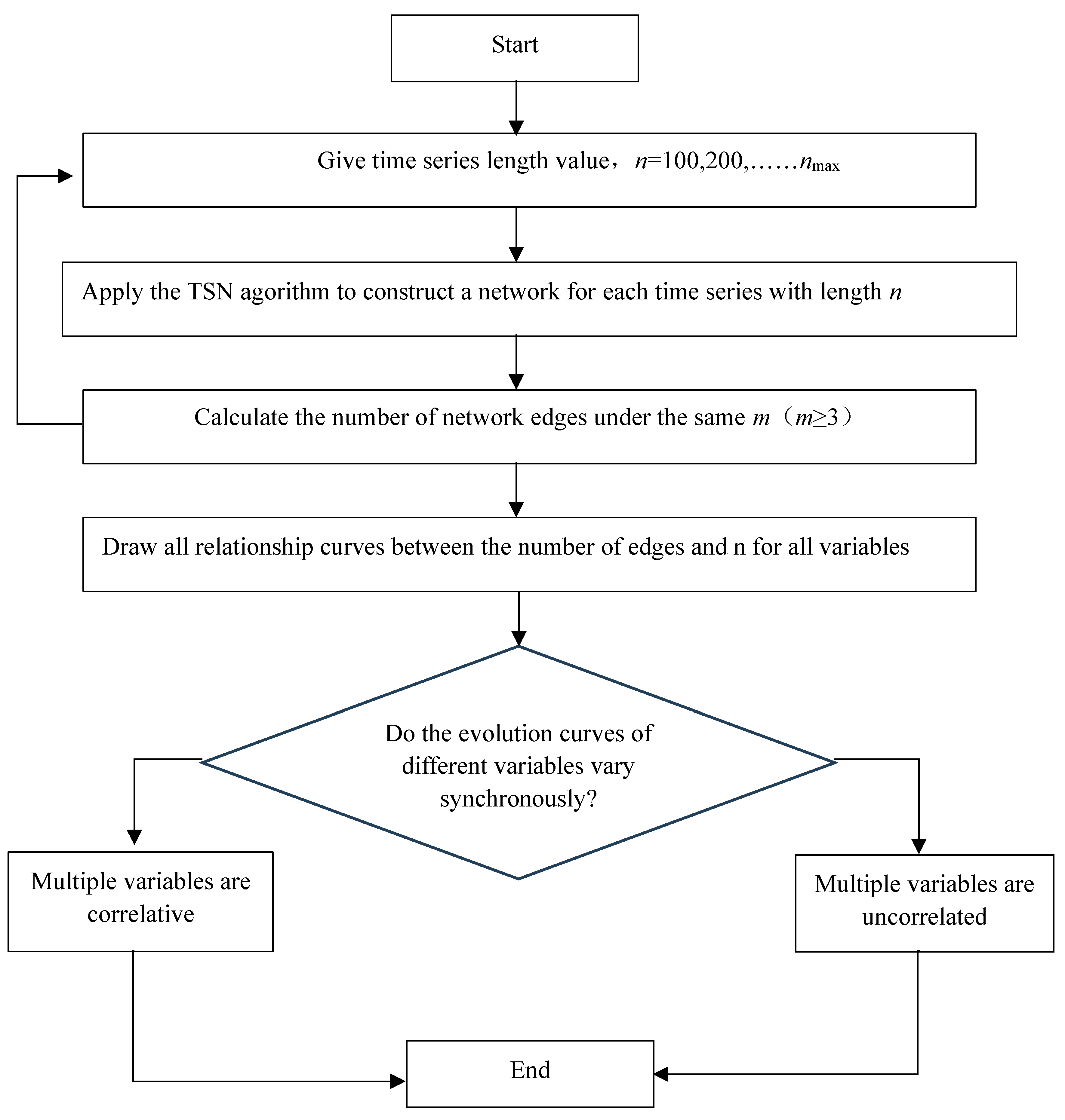
3.6. Flow Chart

The detailed procedure for the judgement of the complicated correlation among multiple time series is shown in Figure 2.

3.7. Novelty of Method

In this study, the judgment method for the complicated correlations among multiple variables (time series) based on NTES is novel.

First, the judgment method for the complicated correlations among multiple variables based on NTES comes from the synchronicity of the dynamic evolution of different variables. Although some scholars have also discussed correlations, NTES reflects the intrinsic dynamic features of the variables evolution, which implies the approximate dynamic orbits of different variables.

Second, our method emphasizes the evolutionary trends of different variables over time. A new feature of NTES is that it shows the changing trend of the number of network edges of different variables when the time series length increases. This method based on time development differs from other current methods for the investigation of multidimensional time series and provides a new observation perspective.

Third, the NTES method uses a visualization approach to reflect the correlation among multiple variables which is not mentioned in existing papers.

4. Numerical Test

4.1. Numerical Experiments

We applied the above method to calculate different series and observed the changing trend in the number of network edges as n increased. First, we compared two independent sequences with the same properties, including two linearly divergent time series, two periodic series, and two chaotic series. Then, we studied two or more variables with a nested structure, including two nested variable sequences for which the correlation coefficient (the correlation coefficient refers to the Pearson’s correlation coefficient in this study) was 1 or −1, two nested variable sequences for which the correlation coefficient was not 1 or −1, mutual nested periodic series including two or more variables, and chaotic time series including two or more variables. Characteristic of all examples are in

Table 1. Numerical experiments.

Type of Example	Description of Example	Number of Example
Two independent time series with the same properties	Linearly divergent time series	EXAMPLE 1
	Periodic series	EXAMPLE 2
	Chaotic series: logistic mapping	EXAMPLE 3
Iterative dynamical system with multiple nested variables	Two variables in one iterative function, the correlation coefficient of the two series is 1 or −1	EXAMPLE 4
	Two variables in one iterative function, the correlation coefficient of the two series is not 1 or −1	EXAMPLE 5
	A nested sequence with period 2	EXAMPLE 6
	A nested sequence with period 4	EXAMPLE 7
	Chaotic time series of the Henon map	EXAMPLE 8
	Chaotic time series of the Lorenz map	EXAMPLE 9
	Chaotic time series of the Rossler map	EXAMPLE 10

.

4.2. Examples

4.2.1. EXAMPLE 1

We provided the two linearly divergent time series shown in Figure 3. For linear series, regardless of how the sequence differed, the network geometric topology was invariant.

As shown in Figure 3, although the values of the two linearly divergent sequences x and y and the function images were different, using the TSN method, the network from either sequence x or y was a tree with the same number of edges. Additionally, as the sequence length n gradually increased, the changing trend of the edges of x and y followed the same pattern. The above results show that, provided it is a linearly divergent sequence, its internal dynamic topological structure is constant. In this study, the internal dynamic topological structure refers to the system spatial diffusion ability and aggregation ability.

4.2.2. EXAMPLE 2

We tested two periodic functions with independent cycles (different cycles). The results are shown in Figure 4.

Here, x = sin(a × t) and y = cos(b × t) with different periods. Although the function values and periods were both different, x and y had the same systematic dynamic characteristics. In the mapped network, the number of network edges of the two variables changed at the same pace.

4.2.3. EXAMPLE 3

We provided a chaotic series. The logistic mapping is shown in Figure 5.

Chaotic systems are sensitive to initial values. However, even if the initial value is changed, and, as a result, the values of the dynamic system change greatly, the dynamic nature of the system does not change. We tested two logistic systems with different initial values. Although the function values of the two logistic sequences were unequal, the chaotic properties were the same because they were obtained using the same iterative equation. The changes in the edges of two logistic sequences in mapped networks were synchronous, that is, the changing trend of the number of edges was the same as n increased.

4.2.4. EXAMPLE 4

Because all variables with nested relationships contain each other in iterative equations and affect each other, they are correlated linearly or nonlinearly. As a result, the relationships are very complicated and cannot be expressed explicitly. We studied the regularity of multiple nested time series as the length of the time series increased as follows.

We provided two variables in one iterative function as given in Equation (4): neither was linearly divergent, but the correlation coefficient of the two series was 1 or −1:

$$\left\{\begin{array}{c}{x}_{t+1}=x_t+y_t\\ y_{t+1}={3x}_t-2y_t\end{array}\right..$$

(4)

The results are shown in Figure 6.

4.2.5. EXAMPLE 5

We provided two variables in one iterative function as given by Equation (5): neither was linearly divergent, but the correlation coefficient of the two series was not 1 or −1:

$$\left\{\begin{array}{c}{x}_{t+1}=x_t+y_t\\ y_{t+1}=x_t-y_t\end{array}\right..$$

(5)

The correlation coefficient was 0.7446 (additionally, 0.8887 at 2000 points and −0.4768 at 1000 points, which changed for different n).

The results are shown in Figure 7.

4.2.6. EXAMPLE 6

A nested sequence with period 2 is:

$$\left\{\begin{array}{c}{x}_{t+1}=x_t+{(-1)}^t{\times \left|x_t-y_t\right|}_{}\\ y_{t+1}=y_t-{(-1)}^{t+1}{\times \left|x_t-y_t\right|}_{}\end{array}\right..$$

(6)

The correlation coefficient is 1.

The results are shown in Figure 8.

4.2.7. EXAMPLE 7

A nested sequence with period 4 is:

$$\left\{\begin{array}{c}{x}_{t+1}={\left(-1\right)}^{t+1}\times \left(x_t-y_t\right)\\ y_{t+1}={\left(-1\right)}^t\times \frac{x_t+y_t}{x_t-y_t} \end{array}.\right.$$

(7)

The correlation coefficient is 0.1576.

The results are shown in Figure 9.

4.2.8. EXAMPLE 8

We studied a chaotic sequence including multiple variables.

In a chaotic dynamic system with two or more variables, the position of the chaotic attractor is determined by multiple variables. The Henon sequence with two variables, the Lorenz sequence with three variables, and the Rossler sequence are given below.

The chaotic time series of the Henon map is described as:

$$\left\{\begin{array}{c}{x\left(t\right)=y(t-1)+1-1.4x(t-1)}^2\\ y\left(t\right)=0.3\ast x(t-1)\end{array}\right..$$

(8)

The Henon map and the results are shown in Figure 10 and Figure 11.

4.2.9. EXAMPLE 9

The chaotic time series of the Lorenz map is described as:

$$\left\{\begin{array}{c}\mathrm{x}\left(t+1\right)=\mathrm{x}\left(t\right)+h\ast (10\ast (\mathrm{y}\left(t\right)-\mathrm{x}\left(t\right)\left)\right)\\ \mathrm{y}\left(t+1\right)=\mathrm{y}\left(t\right)+h\ast \left(-\mathrm{x}\ast \mathrm{z}+28\ast \mathrm{x}\left(t\right)-\mathrm{y}\left(t\right)\right),\\ \mathrm{z}\left(t+1\right)=\mathrm{z}\left(t\right)+h\ast (\mathrm{x}\left(t\right)\ast \mathrm{y}\left(t\right)-\frac{8}{3}\ast \mathrm{z}\left(t\right))\end{array}\right.$$

(9)

where h is the step length.

The Lorenz map and the results are shown in Figure 12 and Figure 13.

For the time series of the Lorenz map, x, y, and z are nested within each other. As the time series length n increases, the change trends exhibited by the three series are essentially the same. This shows that the chaotic nature of the time series of the Lorenz system is stable, and the dynamic properties in the three directions of x, y, and z are similar. However, after n increases above a certain value, the chaotic properties of different time series within the system may change in comparison. As shown on the right of the L line in Graph a, the number of edges of the y sequence begins to be greater than the number of edges of the x sequence, which indicates that the randomness of the x sequence increases more than the randomness of the y sequence, which becomes relatively low, although the evolutionary pace is essentially the same. Additionally, for the Lorenz sequence, we experimented with different m values, and the change trends of x, y, and z were similar under different m values. This shows that our algorithm is stable for the display of the essence of the system under different values of m. Thus, in the following application, it is feasible to set m = 3.

4.2.10. EXAMPLE 10

The chaotic time series of the Rossler map (a = 0.2; b = 0.2; c = 5.7; h = 0.0085) is described in Equation (10):

$$\left\{\begin{array}{c}x\left(t+1\right)=x\left(t\right)+h\ast \left(-1\ast \left(y\left(t\right)+z\left(t\right)\right)\right)\\ y\left(t+1\right)=y\left(t\right)+h\ast \left(x\left(t\right)+a\ast y\left(t\right)\right)\\ z\left(t+1\right)=z\left(t\right)+h\ast \left(b+x\left(t\right)\ast z\left(t\right)-c\ast z\left(t\right)\right)\end{array}\right.$$

(10)

The Rossler map and the results are shown in Figure 14.

For the time series of the Rossler map, x, y, and z are nested within each other. As the time series length n increases, the change trends exhibited by y and z are exactly the same. Although the change trends of the x series compared with those of the y and z series exhibit small, localized differences, they are approximately similar overall. The trends of the three series are essentially similar. For Rossler sequences, we also experimented with different m values, and the change trends of x, y, and z were similar under different values of m. This shows that our algorithm is stable for the display of the essence of the system under different values of m.

4.3. Observations from the Numerical Tests

From the above results, it can be observed that the trend exhibited by the number of edges of the responding network from different variables is the same when the time series length increases within a system either for a periodic dynamic system or a chaotic dynamic system. Even if the embedding dimension m increases as a result of the number of edges decreasing, the evolution trends of the number of edges of the network from different variables in the system remain the same, demonstrating the stability of the algorithm.

The following further summarizes the above results:

(1)

As the number of time points increases, for multiple sequences of the same attribute (e.g., periodic sequences and chaotic sequences) within a system, the changing trend of the number of edges is consistent when time increases.

(2)

For multiple-variable time series, if their iterations are characterized by a nested structure, that is, they affect each other, then, as the length of the time series grows, their changing trends exhibit approximate synchronization overall. Therefore, we obtain a conclusion: if the network edges of multiple-variable time series exhibit an approximate trend over time, their multiple time series are then intrinsically related to each other and correlated.

(3)

Within the same chaotic system, as time increases, the randomness of different variables may change differently, that is, the relative strength of the randomness among different variables changes. Therefore, the number of edges in networks mapped by different variables changes a little differently when the overall change trend is similar. For example, sometimes the x sequence is greater than the y sequence edge in the initial stage, but, over time, the number of edges of the y sequence may become larger than that of the x sequence. In any case, the overall change trends exhibited by the number of edges in the network either mapped by x or y are the same or similar.

4.4. Analysis and Conclusions of the Numerical Experiment

We obtained the following conclusions from the ten examples discussed previously.

From the above results, after two variables (multiple) in a system are mapped in the network, if the edges exhibit the same change trend as the sequence length increases, we can assume that there is a mutually influential relationship between the two (multiple) variables, implying a correlation in the dynamic system iteration. This method does not need to calculate the correlation coefficient, and it works whether the relationship among different variables is linear or nonlinear.

In particular, it should be noted that the related relationship in this study refers to multiple variables, such as x and y, which can be replaced through a certain transformation, even if the transformation that achieves the replacement is too complicated to be expressed. The internal reason for the existence of this transformation is that x and y have the same internal dynamic attributes. Hence, x and y are either a sequence with the same attribute (e.g., both are logistic sequences) or they mutually affect each other through iterative nested relationships. The intrinsic dynamic properties in this study mainly refer to the topological ergodicity and density of space. In the following discussion, we note this as the randomness of the sequence. The most important advantage afforded by the network construction method based on distance that we propose is as follows: the denseness of the dynamic system is combined with topology transferability to observe the overall characteristics of the system dynamic orbit, density is considered, and, then, this dynamic characteristic is expressed by the network topology.

We call the dynamic feature which entails multiple variable sequences exhibiting the same or a similarly changing tendency when the sequence length n increases network topology evolutionary synchronization (NTES). NTES can be used to determine complicated nonlinear correlations among multiple time series.

5. Method Application

We apply the method based on NTES to study the relationship between stock indices and stock trading volume, which is important, and to explain it clearly, as this can help us understand the structure of financial markets and even realize arbitrage. We use NTES to observe the relationship between stock indices and stock trading volume and obtain the following results: we use the Shenzhen stock market, NASDAQ, and SP500 data to study the relationship between stock price indices and trading volume in the three markets. According to the data resources, there are three time series with different lengths of different markets to be studied: NASDAQ from 11 Qctorber 1984 to 15 November 2018, Shenzhen Market from 20 July 1994 to 15 November 2018, and S&P 500 from 3 January 1950 to 15 November 2018.

5.1. NASDAQ Market

Data from NASDAQ Market is used as shown in Figure 15.

Because edges still exist at m = 3 in the network mapped from the series of stock price index and trading volume, both the stock price index and trading volume series are chaotic sequences. Figure 15b shows that the changing trends exhibited by the edges of closing prices and trading volume are synchronized after n becomes greater than 3000, meaning that NTES appears in the NASDAQ market. It is addressed that the closing price and trading volume are correlative and have the same dynamic attributes. After more than 4000 points (on the right of the line L), the number of edges becomes increasingly smaller, a phenomenon which indicates that, after line L, the randomness of the stock price index and trading volume gradually increases.

5.2. Shenzhen Market

Data from Shenzhen Market is used as shown in Figure 16.

Because edges still exist at m = 3 in the network mapped from the series of the stock price index and trading volume, both the stock price index and trading volume series are chaotic sequences. Figure 16b shows that the changing trends exhibited by the edges of the closing prices and trading volume are synchronized after n becomes greater than 1500, meaning that NTES appears in the Shenzhen market. It is addressed that the closing price and trading volume are correlative and have the same dynamic attributes. However, the randomness of the stock price index and trading volume series appears to change. On the right of line L1, the trend exhibited by the number of edges of the price and volume essentially increases as n increases. Additionally, the number of network edges of the trading volume becomes greater than the number of edges in the price network on the right of line L2. The above results indicate that the price and trading volume jointly construct a chaotic system, and, on the right of line L2, the randomness of the price is greater than that of the trading volume.

5.3. S&P 500

Data from S&P 500 is used as shown in Figure 17.

Because of the large time span characterizing S&P 500, to clearly reflect the results only the latter part of the time series is shown in Figure 17a. The S&P 500 index and trading volume series are chaotic sequences. Figure 17b shows that the changing trend exhibited by the closing price and trading volume is approximately synchronous on the right of line L, meaning that NTES appears. Therefore, the closing price and trading volume are regarded as correlative and as having similar attributes. On the right of line L, the changing trend of the number of edges of the price and volume essentially increases as n increases. In the meantime, the number of edges in the volume network is greater than the number of edges in the price network, indicating that the randomness of the price is higher than that of the volume.

5.4. Application Summary

The NTES method was used to study two series of stock price indices and trading volume in three securities markets. Based on the calculations in Section 5.2, the results are summarized as follows:

(1)

Both the stock price index and trading volume series are chaotic sequences because edges still exist at m = 3 in the network mapped from the series of the stock price index and trading volume.

(2)

Because of the existence of NTES, the stock price index and trading volume are regarded as correlative.

(3)

The stock price index and trading volume appear to have different random strengths in different markets and for different lengths of time. Sometimes, the randomness of the price is stronger than the transaction volume, and, sometimes, the transaction volume is stronger than the price. The longer the observed sequence length, the stronger the randomness of the price.

6. Discussion and Conclusions

From the results of the numerical experiment for the proposed method for different securities market data, the following conclusions can be drawn and discussed.

As the length of the time series increases, the changing trends of multiple series exhibit overall approximate synchronization, meaning that NTES exists. NTES demonstrates that multiple time series have similar dynamic properties, are intrinsically related to each other, and are correlative. In fact, the evolution of different variables within a dynamic system is driven by internal forces and external interference forces. If the mutually influential relationship among multiple variables is completely driven by the internal driving force, evolutionary consistency occurs among those variables, with consistency referring to different variables evolving according to the same intrinsic rule. For example, in a chaotic system, such as the Lorenz system, the three variables x, y, and z are defined in one iterative equation. The randomness component and regularity component of the three sequences remain essentially stable. Using the network method in this study, as time goes by (sequence points increase), the number of network edges mapped by different variables essentially evolves at the same or similar pace. Although the randomness of different variables may change with time in a stable chaotic system, the change is small, that is, NTES exists. However, if the undeterminable random component in the external effect exerts different influences on different variables, it causes the difference in the random component between multiple variables to increase. When using the network method in this study, the result is that the number of network edges mapped by different variables cannot change at the same pace over time (i.e., the sequence length increases). At this time, the correlation among multiple variables cannot be determined by each variable, that is, it cannot be assumed that multiple variables are correlative or can be replaced by each other using some type of transformation.

By applying our method, we studied two series that included stock price indices and trading volume in different securities markets and obtained the following inspired conclusions.

There is a complex correlation between stock prices and trading volume. Because both variables are chaotic sequences and random, it is difficult to express their correlation using simple functional relationships. In several studies, researchers have focused on whether the stock price is positively correlated or negatively correlated with the trading volume. Because of the complex relationship between the stock price and transaction volume, it is difficult to provide a clear and analytic relationship, let alone identifying the relationship as positive or negative. In this study, first, we used the TNS method to prove that both the stock price and transaction volume are chaotic sequences. As a chaotic sequence, there is no clear cycle, but there are dense attractors. Our research shows that the two sequences of stock price and trading volume exhibit NTES, that is, the chaotic properties of the two sequences of the stock price and trading volume are similar. Moreover, there are approximate topological transitivity and dense attractors, that is, approximate dynamic orbits. This result inspires us to use the approximation of dynamic orbits to study the relationship between stock prices and trading volume. This is a result not found in the literature.

In addition to finding that the chaotic properties of the two series of stock price and trading volume are similar, we also found that the relative strength of the randomness of the stock price and trading volume can change over time. Therefore, in the study of the correlation between stock price and trading volume series, scholars can investigate the regularity and randomness caused by similar randomness, consider whether the origin of randomness is caused by the system internal dynamics or external random effects, and consider how to divide the difference between the random components and characterize the strength of randomness. These new research possibilities may be the key to revealing the complex correlation between the stock price index and trading volume.

The essence of the proposed method is to describe the properties of different variable sequences based on the dynamic characteristics of different variables in the dynamic system—dynamic characteristics are characterized by topological transitivity and attractor density and are represented by randomness—and characterize it using network topological characteristics. Based on this principle, the correlation strength among different variables is determined. If the evolution of the edge of a network mapped from different variables in a system is essentially the same as the sequence length increases, we consider these two variables to be correlative. Therefore, the smaller the difference between the evolution steps of the number of edges of different variables in a system, the more obvious the NTES. Also, the greater the similarity caused by the correlation of the variables, the greater the difference between the evolution steps of the number of edges of different variables in a system and the larger the randomness impact on different variables from external factors. When the difference is too large, the two variables cannot be considered to be correlative, that is, the interaction between the two variables cannot determine the respective change of the variable sequence and variables cannot replace each other using transformation methods.