Reachable Set Estimation and Controller Design for Linear Time-Delayed Control System with Disturbances

Abstract

This paper investigates reachable set estimation and state-feedback controller design for linear time-delay control systems with bounded disturbances. By constructing an appropriate Lyapunov–Krasovskii functional, we obtain a delay-dependent condition, which determines the admissible bounding ellipsoid for the reachable set of the system we considered. Then, a sufficient condition in the form of liner matrix inequalities is given to solve the problem of controller design and reachable set estimation. Then, by minimizing the volume of the ellipsoid and solving the liner matrix inequality, we obtain the desired ellipsoid and controller gain. A comparative numerical example is given to show the effectiveness of our result.

1. Introduction

The reachable set estimation of dynamic systems is an important research topic in control theory since it has a large number of applications in control systems with actuator saturation [1,2,3], peak-to-peak gain minimization [4], and aircraft collision avoidance [5]. The reachable set of a dynamic system with bounded peak input is defined as the set of system state vectors in the presence of all allowed input disturbances. Reachable set bounding was first considered in the late 1960s in the context of state estimation, and it later received a lot of attention in parameter estimation [6]. Boyd et al. studied the problem of reachable set estimation of linear systems without time delay and obtained an LMI condition for an ellipsoid that bounds the reachable set [7].

It is well known that time delays are extremely common in practice, such as in aircraft, chemical processes, long pipeline supply, belt transmission, extremely complex online analyzers in various industrial systems, and so on. Usually, the occurrence of time delay may lead to instability or performance degradation of dynamic systems [5,8,9,10,11,12]. Therefore, extensive research is devoted to the study of the reachable set estimation issue of dynamic systems with delay. During the past few decades, there have been some excellent results related to the reachable set estimation of time-delay systems [11,13,14,15,16,17,18,19,20,21,22,23,24,25,26,27,28].

In [14], based on the Lyapunov–Razumikhin functional method, Fridman and Shaked first investigated the reachable set estimation of a linear system with time-varying delay and obtained an LMI criteria of an ellipsoid bounding the reachable states set. Kim obtained an improved ellipsoidal bound of a reachable set [16] by using the Lyapunov–Krasovskii functional. Nam and Pathirana obtained a smaller reachable set bound [18] by employing the delay decomposition technique. Zuo et al. obtained a non-ellipsoidal bound of a reachable set of linear time-delayed systems through the maximal Lyapunov functionals and the Razumikhin method [26]. More recently, Zhang et al. investigated the reachable set estimation for uncertain nonlinear systems with time delay [27]. For more references and recent advances in reachable set estimation, one can refer to [29,30,31,32]. The key point of the reachable set estimation is the choice of Lyapunov functional. Motivated by the above idea, we study the reachable set estimation of linear time-delayed control systems with disturbances.

Contributions of this paper are listed below:

• We derived a sufficient condition that determines the admissible bounding ellipsoid for the reachable set related to the delay-dependent system; the condition is in the form of LMI;
• We propose a state feedback controller design method to find the minimum ellipsoidal bound so that the reachable set of the resulting closed-loop system is bounded by an ellipsoid, and the admissible ellipsoid should be as small as possible;
• We show that our conclusion is an extension of the available results in the paper [16].

In this paper, we intend to design a state feedback controller so that the reachable set of the resulting closed-loop system is contained in an admissible ellipsoid, and the admissible ellipsoid should be as small as possible. The rest of this paper is organized as follows: In Section 2, in order to obtain the main result, some useful lemmas and preliminary knowledge are given. In Section 3, by constructing an appropriate Lyapunov–Krasovskii functional, we obtain a condition related to delay-dependent, which determines the admissible bounding ellipsoid for the reachable set of the system we considered. Then, a sufficient condition in the form of liner matrix inequalities is given to solve the problem of controller design with reachable set estimation. Finally, by minimizing the volume of the ellipsoid and solving the liner matrix inequality, we obtain the desired ellipsoid and controller gain. Section 4 presents a comparative numerical example to show the effectiveness of the proposed methods.

Notation

Throughout this paper, the notations are standard. ${\mathbb{R}}^n$ is the vector of real numbers, ${\mathbb{R}}^{n\times m}$ is the $n\times m$ real matrix, I is the identity matrix, 0 is the zero matrix, and $A^T$ presents the transpose of A. For a matrix P, $P>0$ denotes P as a symmetric positive definite matrix; also, $x_t\left(\theta \right)=x(t+\theta ),\theta \in [-h,0]$, and symbol $(★)$ in a matrix represents the symmetric part.

2. Problem Statement and Preliminaries

Consider the following linear time-delay control system with bounded disturbances:

$$\left\{\begin{array}{cc}\dot{x}\left(t\right)=Ax\left(t\right)+Dx(t-d\left(t\right))+Bu\left(t\right)+Ew\left(t\right),\hfill & \\ x\left(t\right)\equiv 0,t\in [-h,0],\hfill \end{array}\right.$$

(1)

where $x\left(t\right)\in {\mathbb{R}}^n$ is the state vector, $u\left(t\right)$ is the control vector, $A\in {\mathbb{R}}^{n\times n}, D\in {\mathbb{R}}^{n\times n}, B\in {\mathbb{R}}^{n\times n}$, and $E\in {\mathbb{R}}^{n\times m},A,D,B$, and E are constant matrices, $w\left(t\right)\in {\mathbb{R}}^m$ is the disturbance, satisfying

$$w^T\left(t\right)w\left(t\right)\le w_m^2$$

(2)

and $d\left(t\right)$ is a time-varying delay, satisfying

$$0\le d\left(t\right)\le h,\left|\dot{d}\left(t\right)\right|\le u\le 1$$

(3)

where $w_m, d$, and u are constants.

In this paper, based on the modified Lyapunov–Krasovskii functional, which is used for exponential stability analysis in [33,34], we intend to design a state feedback controller $K, G$, that is $u\left(t\right)=Kx\left(t\right)+Gx(t-d(t\left)\right)$, such that the reachable set of the closed-loop system

$$\dot{x}\left(t\right)=(A+BK)x\left(t\right)+(D+BG)x(t-d\left(t\right))+Ew\left(t\right)$$

(4)

is bounded by an ellipsoid $\epsilon (P,1)$:

$$\epsilon (P,1)=\left\{x\in {\mathbb{R}}^n:x^{T}Px\le 1, P>0\right\}$$

(5)

The reachable set of system (4) is denoted as follows:

$$R_x=\left\{x\left(t\right)\left|x\left(t\right)andw\left(t\right)satisfy\left(2\right)and\left(3\right), t\ge 0\right.\right\}$$

The following three useful lemmas are given to derive the main results.

Lemma 1 

([35]). The following relation is known as the Leibniz rule

$$\frac{d}{dt}{\int }_{b\left(t\right)}^{a\left(t\right)}f(t,s)ds=\dot{a}\left(t\right)f[t,a\left(t\right)]-\dot{b}\left(t\right)f[t,b\left(t\right)]+{\int }_{b\left(t\right)}^{a\left(t\right)}\frac{\delta }{\delta t}f(t,s)ds.$$

Lemma 2 

([36]). For any constant matrix $Q=Q^T>0$, we have

$$-{\int }_{t-d\left(t\right)}^t{\dot{x}}^T\left(s\right)Q{\dot{x}}^T\left(s\right)ds\le [x^T\left(t\right),x^T(t-d\left(t\right))]\left[\begin{array}{cc}-Q& Q\\ Q& -Q\end{array}\right]{[x^T\left(t\right),x^T(t-d\left(t\right))]}^T.$$

Lemma 3 

([7]). Let Q be a symmetric positive definite matrix. For any matrices $P, S$ with appropriate dimensions, where $P=P^T$, then

$$\left[\begin{array}{cc}P& S\\ S^T& Q\end{array}\right]>0$$

if and only if $P-S{Q}^{-1}{S}^T>0$.

Lemma 4 

([7]). Let $V\left(x\right(0\left)\right)=0$ and $w^T\left(t\right)w\left(t\right)\le w_m^2$, if $\dot{V}\left(x_t\right)+\alpha V\left(x_t\right)-\beta w^T\left(t\right)w\left(t\right)\le 0, \alpha >0, \beta >0$, then we have $V\left(x_t\right)\le \frac{\beta }{\alpha }{w}_m^2,\forall t>0$.

3. Main Results

Theorem 1. 

For given scalars $h,u>0$, if there exist matrices $L,H\in {\mathbb{R}}^{1\times n},\overline{M},\tilde{P},\tilde{R},\tilde{S},\tilde{W},\tilde{X},\tilde{Y},\tilde{Z},\widehat{R},\widehat{Z},\breve{Z}\in {\mathbb{R}}^{n\times n}$ with $\overline{M},\tilde{R},\tilde{S},\tilde{W},\tilde{X}>0$ and a scalar $\alpha >0$ such that they satisfy the following matrix inequalities:

$$\begin{array}{cc}\hfill & \left[\begin{array}{ccccc}{\overline{\Phi }}_{11}& D\overline{M}+BH-\tilde{Y}& \overline{M}{A}^T+L^T{B}^T+\breve{Z}+\alpha \overline{M}& E& \tilde{Y}\\ ★& -(1-u)e^{-\alpha h}\tilde{S}+u^2\tilde{W}& \overline{M}D+H^T{B}^T-\breve{Z}& 0& 0\\ ★& ★& -\frac{1}{h}{e}^{-\alpha h}\widehat{R}+\alpha \widehat{Z}& E& {\breve{Z}}^T\\ ★& ★& ★& \frac{-\alpha }{w_m^2}& 0\\ ★& ★& ★& ★& -\tilde{W}\end{array}\right]\le 0,\hfill \end{array}$$

(6)

$$\begin{array}{cc}\hfill & \left[\begin{array}{cc}\overline{M}-\tilde{P}& \tilde{Y}\\ ★& \tilde{Z}+\frac{1}{h}{e}^{-\alpha h}\tilde{S}\end{array}\right]\ge 0,\hfill \end{array}$$

(7)

where ${\overline{\Phi }}_{11}=A\overline{M}+BL+\overline{M}{A}^T+L^T{B}^T+\alpha \overline{M}+\tilde{Y}+{\tilde{Y}}^T+\tilde{S}+h\tilde{R}$, then the reachable sets of the system (4) are bounded by an ellipsoid $\epsilon (P,1)$ defined in (5). At this point, the state feedback gain is $K=L{\overline{M}}^{-1}, G=H{\overline{M}}^{-1}$.

Proof. 

To prove this theorem, let us consider the following Lyapunov–Krasovskii function:

$$V\left(x_t\right)=V_1\left(x_t\right)+V_2\left(x_t\right)+V_3\left(x_t\right),$$

(8)

where

$$\begin{array}{cc}\hfill & V_1\left(x_t\right)=x^T\left(t\right)Px\left(t\right),\hfill \\ \hfill & V_2\left(x_t\right)={\int }_{t-d\left(t\right)}^t{e}^{-\alpha (s-t)}[x^T\left(s\right)Sx\left(s\right)+(h-t+s)x^T\left(s\right)Rx\left(s\right)]ds,\hfill \\ \hfill & V_3\left(x_t\right)=\left[\begin{array}{cc}{x}^T\left(t\right)& {\eta }^T\left(t\right)\end{array}\right]\left[\begin{array}{cc}X& Y\\ ★& Z\end{array}\right]\left[\begin{array}{c}x\left(t\right)\\ \eta \left(t\right)\end{array}\right],\hfill \\ \hfill & \eta \left(t\right)={\int }_{t-d\left(t\right)}^{t}x\left(s\right)ds,\hfill \end{array}$$

where $P,S,R,X,Y,Z$ are symmetric matrices with appropriate dimensions. First, we prove that $V\left(x_t\right)$ in (8) is a good Lyapunov–Krasovskii functional candidate. For $t-d\left(t\right)\le s\le t$ and $0\le d\left(t\right)\le h$, we can get $e^{-h}\le e^{-d\left(t\right)}\le e^{s-t}\le 1$ and $0\le h-d\left(t\right)\le h-t+s\le h$. In the light of the Lamma 2, we have

$$V_2\left(x_t\right)\ge {\int }_{t-d\left(t\right)}^t{e}^{-\alpha (s-t)}{x}^T\left(s\right)Sx\left(s\right)ds\ge \frac{1}{h}{e}^{-\alpha h}{\eta }^T\left(t\right)S\eta \left(t\right),$$

then

$$V_2\left(x_t\right)+V_3\left(x_t\right)\ge \left[\begin{array}{cc}{x}^T\left(t\right)& {\eta }^T\left(t\right)\end{array}\right]\left[\begin{array}{cc}X& Y\\ ★& Z+\frac{1}{h}{e}^{-\alpha h}S\end{array}\right]\left[\begin{array}{c}x\left(t\right)\\ \eta \left(t\right)\end{array}\right].$$

If

$$\left[\begin{array}{cc}X& Y\\ ★& Z+\frac{1}{h}{e}^{-\alpha h}S\end{array}\right]\ge 0,$$

(9)

then we have $V_2\left(x_t\right)+V_3\left(x_t\right)\ge 0$.

Hence, we have

$$\left\{\begin{array}{cc}V\left(x_t\right)=V_1\left(x_t\right)+V_2\left(x_t\right)+V_3\left(x_t\right)\ge V_1\left(x_t\right)=x^T\left(t\right)Px\left(t\right),\hfill & \\ V\left(x_t\right)=0,whenx\left(s\right)=0,\forall s\in [t-d\left(t\right),t],\hfill \end{array}\right.$$

(10)

which shows $V\left(x_t\right)$ in (8) is an L–K functional.

Next, from Lemma 1, we obtain the following time derivatives:

$$\begin{array}{cc}\hfill & {\displaystyle \frac{d}{dt}}{V}_1\left(x_t\right)=2x^T\left(t\right)P[(A+BK)x\left(t\right)+(D+BG)x(t-d\left(t\right))+Ew\left(t\right)],\hfill \end{array}$$

(11)

$$\begin{array}{cc}\hfill & {\displaystyle \frac{d}{dt}}{V}_2\left(x_t\right)=x^T\left(t\right)(S+hR)x\left(t\right)-(1-\dot{d}\left(t\right))e^{-\alpha d\left(t\right)}{x}^T(t-d\left(t\right))Sx(t-d\left(t\right))\hfill \\ \hfill & -(1-\dot{d}\left(t\right))e^{-\alpha d\left(t\right)}(h-d\left(t\right))x^T(t-d\left(t\right))Rx(t-d\left(t\right))\hfill \\ \hfill & -{\int }_{t-d\left(t\right)}^t{e}^{-\alpha (s-t)}{x}^T\left(s\right)Rx\left(s\right)ds-\alpha V_2\left(x_t\right)\hfill \\ \hfill & \le x^T\left(t\right)(S+hR)x\left(t\right)-(1-u)e^{-\alpha h}{x}^T(t-d\left(t\right))Sx(t-d\left(t\right))\hfill \\ \hfill & -\frac{1}{h}{e}^{-\alpha h}{\eta }^T\left(t\right)R\eta \left(t\right)-\alpha V_2\left(x_t\right),\hfill \end{array}$$

(12)

$$\begin{array}{cc}\hfill & {\displaystyle \frac{d}{dt}}{V}_3\left(x_t\right)=2\left[\begin{array}{cc}{x}^T\left(t\right)& {\eta }^T\left(t\right)\end{array}\right]\left[\begin{array}{cc}X& Y\\ ★& Z\end{array}\right]\left[\begin{array}{c}\dot{x}\left(t\right)\\ \left(x\right(t)-x(t-d\left(t\right))\end{array}\right]\hfill \\ \hfill & +2\dot{d}\left[\begin{array}{cc}{x}^T\left(t\right)& {\eta }^T\left(t\right)\end{array}\right]\left[\begin{array}{c}Y\\ Z\end{array}\right]x(t-d\left(t\right))\hfill \\ \hfill & \le 2\left[\begin{array}{cc}{x}^T\left(t\right)& {\eta }^T\left(t\right)\end{array}\right]\left[\begin{array}{cc}X& Y\\ ★& Z\end{array}\right]\left[\begin{array}{c}(A+BK)x\left(t\right)+(D+BG)x(t-d(t\left)\right)+Ew\left(t\right)\\ x\left(t\right)-x(t-d(t\left)\right)\end{array}\right]\hfill \\ \hfill & +\left[\begin{array}{cc}{x}^T\left(t\right)& {\eta }^T\left(t\right)\end{array}\right]\left[\begin{array}{c}Y\\ Z\end{array}\right]W^{-1}\left[\begin{array}{cc}{Y}^T& Z^T\end{array}\right]\left[\begin{array}{c}x\left(t\right)\\ \eta \left(t\right)\end{array}\right]+u^2{x}^T(t-d\left(t\right))Wx(t-d\left(t\right)),\hfill \end{array}$$

(13)

where we used the relation that $2a^{T}b\le a^T{W}^{-1}a+b^{T}Wb, W>0$ and the constraints (2) and (3) in the derivation of the inequality (13).

Through (9) and (11)–(13), we obtain:

$$\begin{array}{cc}\dot{V}\left(x_t\right)+\alpha V\left(x_t\right)-\beta w^T\left(t\right)w\left(t\right)\hfill & \\ \le {\xi }_t^T\left(\Omega +\left[\begin{array}{c}{Y}^T\\ 0\\ Z^T\\ 0\end{array}\right]W^{-1}\left[\begin{array}{cccc}{Y}^T& 0& Z^T& 0\end{array}\right]\right){\xi }_t\hfill & \\ :={\xi }_t^T\Psi {\xi }_t,\hfill \end{array}$$

where

$${\xi }_t^T=\left[x^T\left(t\right)x^T(t-d\left(t\right)){\eta }^T\left(t\right)w^T\left(t\right)\right],$$

$$\Omega =\left[\begin{array}{cccc}{\varphi }_{11}& (P+X)(D+BG)-Y& {(A+BK)}^{T}Y+Z+\alpha Y& (P+X)E\\ ★& -(1-u)e^{-\alpha h}S+u^{2}W& {(D+BG)}^{T}Y-Z& 0\\ ★& ★& -\frac{1}{h}{e}^{-\alpha h}+\alpha Z& Y^{T}E\\ ★& ★& ★& \frac{-\alpha }{w_m^2}\end{array}\right]$$

and

${\varphi }_{11}=(P+X)(A+BK)+{(A+BK)}^T(P+X)+\alpha (P+X)+Y+Y^T+S+hR$.

If $\Psi \le 0$, by virtue of Lamma 3, we get

$$\left[\begin{array}{ccccc}{\Phi }_{11}& M(D+BG)-Y& {(A+BK)}^{T}Y+Z+\alpha Y& ME& Y\\ ★& -(1-u)e^{-\alpha h}S+u^{2}W& {(D+BG)}^{T}Y-Z& 0& 0\\ ★& ★& -\frac{1}{h}{e}^{-\alpha h}+\alpha Z& Y^{T}E& Z\\ ★& ★& ★& \frac{-\alpha }{w_m^2}& 0\\ ★& ★& ★& ★& -W\end{array}\right]\le 0,$$

(14)

where

$M=P+X$, ${\Phi }_{11}=M(A+BK)+{(A+BK)}^{T}M+\alpha M+Y+Y^T+S+hR$.

By defining $N_1=diag(M^{-1};M^{-1};Y^{-1};I;M^{-1})$, pre- and post-multiplying the inequality (14) by $N_1$ and $N_1^T$, and defining $\overline{M}=M^{-1}$, $L=K{M}^{-1}$, $H=G{M}^{-1}$, $\tilde{X}=M^{-1}X{M}^{-1}$, $\tilde{Y}=M^{-1}Y{M}^{-1}$, $\tilde{R}=M^{-1}R{M}^{-1}$, $\tilde{Z}=M^{-1}Z{M}^{-1}$, $\tilde{S}=M^{-1}S{M}^{-1}$, $\tilde{W}=M^{-1}W{M}^{-1}$, $\breve{Z}=M^{-1}Z{Y}^{-1}$, $\widehat{R}=Y^{-1}R{Y}^{-1}$, $\widehat{Z}=Y^{-1}Z{Y}^{-1}$, the following inequality is derived:

$$\left[\begin{array}{ccccc}{\overline{\Phi }}_{11}& D\overline{M}+BH-\tilde{Y}& \overline{M}{A}^T+L^T{B}^T+\breve{Z}+\alpha \overline{M}& E& \tilde{Y}\\ ★& -(1-u)e^{-\alpha h}\tilde{S}+u^2\tilde{W}& \overline{M}D+H^T{B}^T-\breve{Z}& 0& 0\\ ★& ★& -\frac{1}{h}{e}^{-\alpha h}\widehat{R}+\alpha \widehat{Z}& E& {\breve{Z}}^T\\ ★& ★& ★& \frac{-\alpha }{w_m^2}& 0\\ ★& ★& ★& ★& -\tilde{W}\end{array}\right]\le 0,$$

(15)

where $\overline{M}={(P+X)}^{-1}$, ${\overline{\Phi }}_{11}=A\overline{M}+BL+\overline{M}{A}^T+L^T{B}^T+\alpha \overline{M}+\tilde{Y}+{\tilde{Y}}^T+\tilde{S}+h\tilde{R}$. Thus, if inequality (15) holds, we have

$$\dot{V}\left(x_t\right)+\alpha V\left(x_t\right)-\frac{\alpha }{w_m^2}{w}^T\left(t\right)w\left(t\right)\le 0.$$

which means, by virtue of Lemma 4, that $V\left(x_t\right)=V_1\left(x_t\right)+V_2\left(x_t\right)+V_3\left(x_t\right)\le 1$. Since $V_2\left(x_t\right)+V_3\left(x_t\right)\ge 0$, from inequality (9), we get $V_1\left(x_t\right)=x^T\left(t\right)Px\left(t\right)\le 1$. Following a similar line, we need to convert condition (9) into

$$\left[\begin{array}{cc}M-P& Y\\ ★& Z+\frac{1}{h}{e}^{-\alpha h}S\end{array}\right]\ge 0$$

(16)

By defining $N_2=diag(M^{-1};M^{-1})$ and pre- and post-multiplying the inequality (16) by $N_2$ and $N_2^T$, the following inequality is derived:

$$\left[\begin{array}{cc}\overline{M}-\tilde{P}& \tilde{Y}\\ ★& \tilde{Z}+\frac{1}{h}{e}^{-\alpha h}\tilde{S}\end{array}\right]\ge 0$$

(17)

which completes the proof. This implies that the reachable sets of the closed-loop system in (4) are bounded by the ellipsoid $\epsilon (P,1)$ defined in (5), and the desired state-feedback controller can be obtained as $K=L{\overline{M}}^{-1},G=H{\overline{M}}^{-1}$. □

Remark 1. 

The L–K functional (8) is a function of the system state and control input, with certain positive definite and sub-positive definite conditions. With this function, the stability of time-delay systems can be determined, error bounds can be estimated, and control strategies can be designed to ensure system stability.

Remark 2. 

In order to obtain the ‘smallest’ possible bound for the reachable set, we introduce the method in [14,16]. That is, maximize δ subject to $\delta I\le P$, which can be transformed to the following optimization problem for a scalar $\delta >0$:

$$\left\{\begin{array}{cc}min\overline{\delta },(\overline{\delta }=\frac{1}{\delta })\hfill & \\ s.t\left[\begin{array}{cc}\overline{\delta }& I\\ I& P\end{array}\right]\ge 0.\hfill \end{array}\right.$$

(18)

Then, by defining $N_3=diag(I;\overline{M})$, pre- and post-multiplying inequality (18) by $N_3$ and $N_3^T$, and defining $\tilde{P}=\overline{M}P\overline{M}$, the following optimization is derived:

$$\left\{\begin{array}{cc}min\overline{\delta },(\overline{\delta }=\frac{1}{\delta })\hfill & \\ s.t\left[\begin{array}{cc}\overline{\delta }& \overline{M}\\ \overline{M}& \tilde{P}\end{array}\right]\ge 0.\hfill \end{array}\right.$$

(19)

Therefore, we can obtain the ‘smallest’ possible bound for the reachable set of the system (4) by solving the following optimization problem for a scalar $\delta >0$:

$$\begin{array}{cc}min\overline{\delta },(\overline{\delta }=\frac{1}{\delta })\hfill & \\ s.t\left\{\begin{array}{cc}\left(a\right)\left[\begin{array}{cc}\overline{\delta }& \overline{M}\\ \overline{M}& \tilde{P}\end{array}\right]\ge 0,\hfill & \\ \left(b\right)\left(6\right),\left(7\right)or\left(15\right),\left(17\right).\hfill \end{array}\right.\hfill \end{array}$$

(20)

Remark 3. 

In [16], for given scalars $h,u>0$, if there exist matrices $P,S,R,W,X,Y,Z\in {\mathbb{R}}^{n\times n}$ with $P,S,R,W>0$ and a scalar $\alpha >0$, they satisfy the following matrix inequalities:

$$\begin{array}{ccc}\hfill & \left[\begin{array}{ccccc}{\Phi }_{11}& (P+X)D-Y& A^{T}Y+Z+\alpha Y& (P+X)E& Y\\ ★& -(1-u)e^{-\alpha h}S+u^{2}W& D^{T}Y-Z& 0& 0\\ ★& ★& -\frac{1}{h}{e}^{-\alpha h}+\alpha Z& Y^{T}E& Z\\ ★& ★& ★& \frac{-\alpha }{w_m^2}& 0\\ ★& ★& ★& ★& -W\end{array}\right]\hfill & \hfill \le 0,\end{array}$$

(21)

$$\begin{array}{cc}\hfill & \left[\begin{array}{cc}X& Y\\ ★& Z+\frac{1}{h}{e}^{-\alpha h}S\end{array}\right]\ge 0,\hfill \end{array}$$

(22)

where ${\Phi }_{11}=(P+X)A+A^T(P+X)+\alpha (P+X)+Y+Y^T+S+hR$.

To find the ‘smallest’ bound for the reachable set, one may propose a simple optimization problem. That is, maximize $\delta$ subject to $\delta I\le P$, which can be transformed to the following optimization problem for a scalar $\delta >0$:

$$\begin{array}{cc}min\overline{\delta },(\overline{\delta }=\frac{1}{\delta })\hfill & \\ s.t\left\{\begin{array}{cc}\left(a\right)\left[\begin{array}{cc}\overline{\delta }& I\\ I& P\end{array}\right]\ge 0,\hfill & \\ \left(b\right)\left(21\right),\left(22\right).\hfill \end{array}\right.\hfill \end{array}$$

(23)

Remark 4. 

If $B=0,K=0$, and $G=0$ in (6) and (7) of Theorem 1, the condition becomes the condition in [16], and (20) also becomes (23) in Remark 2; in this respect, the conclusion can be seen as an extension of [16].

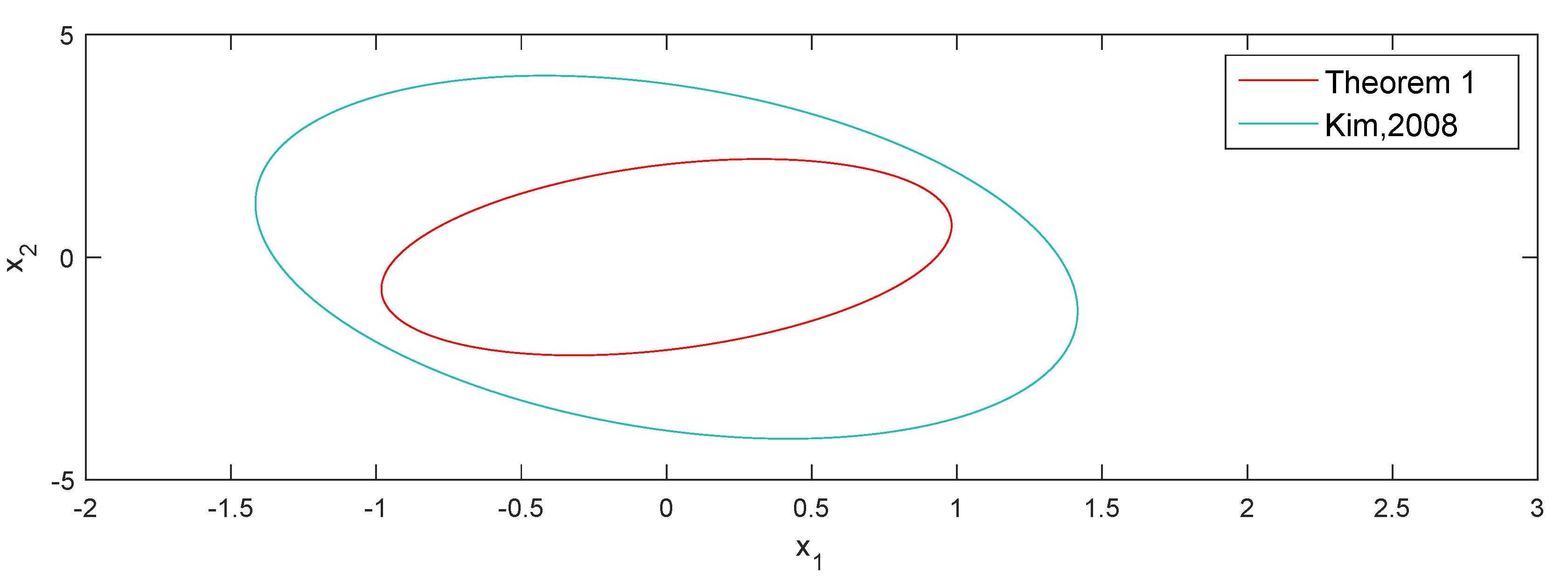
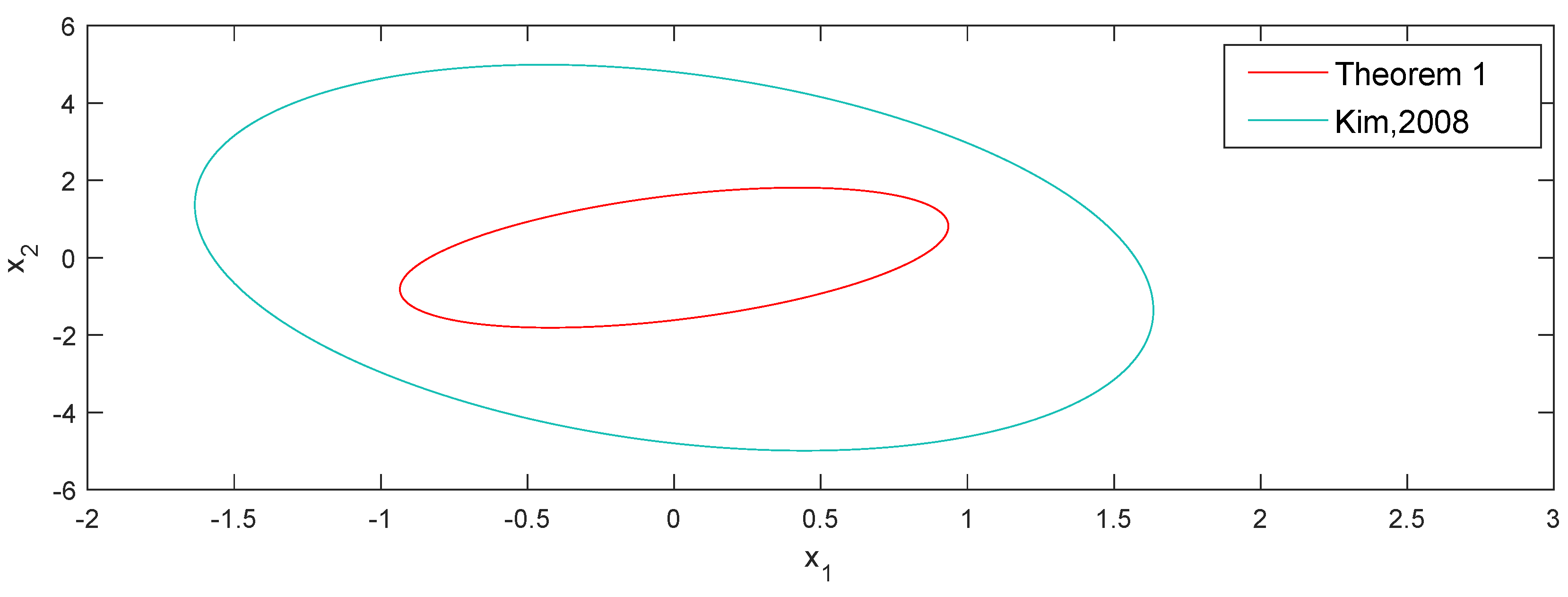
4. Numerical Example

An example is presented to illustrate our proposed method. The simulation is performed on Matlab and by using the LMI toolbox, a package for specifying and solving linear matrix inequalities.

Consider the linear state-delayed control system (1) with the following parameters

$$A=\left[\begin{array}{cc}-2& 0\\ 0& -0.9\end{array}\right], D=\left[\begin{array}{cc}-1& 0\\ -1& -1\end{array}\right], B=\left[\begin{array}{c}1\\ 1\end{array}\right], E=\left[\begin{array}{c}-0.5\\ 1\end{array}\right], w_m=1.$$

By solving optimization problem (20), we get the sizes of the ellipsoidal bound of a reachable set for various u when $h=0.70$ and $h=0.75$. These results are summarized in

Table 1. Computed $\overline{\delta }$’s in Example for $0\le d\left(t\right)\le 0.7,\left|\dot{d}\left(t\right)\right|\le u\le 1$.

Method	u
	0	0.1	0.2	0.3	0.4	0.5	0.6
[16]	2.2586	2.4970	2.8497	3.4355	4.5384	7.0915	16.8263
Theorem 1	1.4571	1.6372	1.8905	2.2702	2.9171	4.2496	8.1427

and

Table 2. Computed $\overline{\delta }$’s in Example for $0\le d\left(t\right)\le 0.75,\left|\dot{d}\left(t\right)\right|\le u\le 1$.

Method	u
	0	0.1	0.2	0.3	0.4	0.5	0.6
[16]	2.5077	2.8071	3.2462	3.9935	5.4419	8.9945	25.1048
Theorem 1	1.6222	1.8417	2.1363	2.5992	3.4134	5.1046	10.4056

; figures are also provided in Figure 1 and Figure 2. The results of our method and the method in [16] are compared.

As can be seen in Table 1, when $h=0.7,u=0.6$, our results greatly reduce the size of the ellipsoid. At this point, the state feedback gain is $K=[-0.5209-1.3698],$$G=[0.9414-0.4495]$.

It is obvious that the results of this paper are better than the autonomous systems in [16], which shows the effectiveness of our method.

5. Conclusions

In this paper, we deal with the problem of reachable set estimation and state-feedback controller design for linear time-delay control systems with bounded disturbances. Firstly, by constructing an appropriate L–K functional, we obtained a delay-dependent condition, which determines the admissible bounding ellipsoid for the reachable set of the system we considered. Secondly, a sufficient condition in form of liner matrix inequalities is given to solve the problem of controller design with reachable set estimation. Finally, by minimizing the volume of the ellipsoid and solving the liner matrix inequality, we obtain the desired ellipsoid and controller gain. The numerical example shows that the results of the method in this paper are better than that in [16] for the autonomous systems in [16], which shows the effectiveness of the proposed method.

References

1. Hu, T.; Lin, Z. Control Systems with Actuator Saturation: Analysis and Design; Springer Science & Business Media: Berlin/Heidelberg, Germany, 2001. [Google Scholar]
2. Hu, T.; Teel, A.R.; Zaccarian, L. Stability and performance for saturated systems via quadratic and nonquadratic Lyapunov functions. IEEE Trans. Autom. Control 2006, 51, 1770–1786. [Google Scholar] [CrossRef]
3. Kim, J.-H.; Jabbari, F. Scheduled controllers for buildings under seismic excitation with limited actuator capacity. J. Eng. Mech. 2004, 130, 800–808. [Google Scholar] [CrossRef]
4. Abedor, J.; Nagpal, K.; Poola, K. A linear matrix inequality approach to peak-to-peak minimization. Int. J. Robust Nonlinear Control 1996, 6, 899–927. [Google Scholar] [CrossRef]
5. Hwang, I.; Stipanovic, D.M.; Tomlin, C.J. Applications of polytopic approximations of reachable sets to linear dynamic games and a class of nonlinear systems. In Proceedings of the American Control Conference, Denver, CO, USA, 4–6 June 2003; pp. 4613–4619. [Google Scholar]
6. Durieu, C.; Walter, E.; Polyak, B. Multi-input multi-output ellipsoidal state bounding. J. Optim. Theory Appl. 2001, 111, 273–303. [Google Scholar] [CrossRef]
7. Boyd, S.; El Ghaoui, L.; Feron, E.; Balakrishnan, V. Linear Matrix Inequalities in Systems and Control Theory; SIAM: Philadelphia, PA, USA, 1994. [Google Scholar]
8. Gao, H.; Chen, T. New results on stability of discrete-time systems with time-varying state delay. IEEE Trans. Autom. Control 2007, 52, 328–334. [Google Scholar] [CrossRef]
9. Kwon, O.M.; Lee, S.M.; Park, J.H. Stability for neural networks with time-varying delays via some new approaches. IEEE Trans. Neural Netw. Learn. Syst 2013, 24, 181–193. [Google Scholar] [CrossRef] [PubMed]
10. Shi, L.; Zhu, H.; Zhong, S.; Hou, L. Globally exponential stability for neural networks with time-varying delays. Appl. Math. Comput. 2013, 219, 10487–10498. [Google Scholar] [CrossRef]
11. Xu, S.; Lam, J. Improved delay-dependent stability criteria for time-delay systems. IEEE Trans. Autom. Control 2005, 50, 384–387. [Google Scholar]
12. Xiao, N.; Jia, Y. New approaches on stability criteria for neural networks with two additive time-varying delay components. Neurocomputing 2013, 118, 150–156. [Google Scholar] [CrossRef]
13. Chen, H.; Zhong, S. New results on reachable set bounding for linear time delay systems with polytopic uncertainties via novel inequalities. J. Inequalities Appl. 2017, 2017, 2346–2350. [Google Scholar] [CrossRef]
14. Fridman, E.; Shaked, U. On reachable sets for linear systems with delay and bounded peak inputs. Automatica 2003, 39, 2005–2010. [Google Scholar] [CrossRef]
15. Feng, Z.; Zheng, W.X. On reachable set estimation of delay Markovian jump systems with partially known transition probabilities. J. Frankl. Inst. 2016, 353, 3835–3856. [Google Scholar] [CrossRef]
16. Kim, J.H. Improved ellipsoidal bound of reachable sets for time-delayed linear systems with disturbances. Automatica 2008, 44, 2940–2943. [Google Scholar] [CrossRef]
17. Kwon, O.M.; Lee, S.M.; Park, J.H. On the reachable set bounding of uncertain dynamic systems with time-varying delays and disturbances. Inf. Sci. 2011, 181, 3735–3748. [Google Scholar] [CrossRef]
18. Nam, P.T.; Pathirana, P.N. Further result on reachable set bounding for linear uncertain polytopic systems with interval time-varying delays. Automatica 2011, 47, 1838–1841. [Google Scholar] [CrossRef]
19. Shen, C.; Zhong, S. The ellipsoidal bound of reachable sets for linear neutral systems with disturbances. J. Frankl. Inst. 2011, 348, 2570–2585. [Google Scholar] [CrossRef]
20. Sheng, Y.; Shen, Y. Improved reachable set bounding for linear time-delay systems with disturbances. J. Frankl. Inst. 2016, 353, 2708–2721. [Google Scholar] [CrossRef]
21. Wang, W.; Zhong, S.; Liu, F.; Cheng, J. Reachable set estimation for linear systems with time-varying delay and polytopic uncertainties. J. Frankl. Inst. 2019, 356, 7322–7346. [Google Scholar] [CrossRef]
22. Zuo, Z.; Ho, D.W.C.; Wang, Y. Reachable set bounding for delayed systems with polytopic uncertainties: The maximal Lyapunov–Krasovskii functional approach. Automatica 2010, 46, 949–952. [Google Scholar] [CrossRef]
23. Zuo, Z.; Ho, D.W.C.; Wang, Y. Reachable set estimation for linear systems in the presence of both discrete and distributed delays. IET Control Theory Appl. 2011, 5, 1808–1812. [Google Scholar] [CrossRef]
24. Zuo, Z.; Wang, Y. Results on reachable set estimation for linear systems with both discrete and distributed delays. IET Control Theory Appl. 2012, 6, 2346–2350. [Google Scholar] [CrossRef]
25. Zuo, Z.; Chen, Y.; Wang, Y.; Ho, D.W.C.; Chen, M.Z.Q.; Li, H. A note on reachable set bounding for delayed systems with polytopic uncertainties. J. Frankl. Inst. 2013, 350, 1827–1835. [Google Scholar] [CrossRef]
26. Zuo, Z.; Wang, Z.; Chen, Y.; Wang, Y. A non-ellipsoidal reachable set estimation for uncertain neural networks with time-varying delay. Commun. Nonlinear Sci. Numer. Simulat. 2014, 19, 1097–1106. [Google Scholar] [CrossRef]
27. Zhang, Z.; Wang, X.; Xie, W.; Shen, Y. Reachable set estimation for uncertain nonlinear systems with time delay. Optim. Control Appl. Methods. 2020, 41, 1644–1656. [Google Scholar] [CrossRef]
28. Zhang, L.; Feng, Z.; Jiang, Z.; Zhao, N.; Yang, Y. Improved results on reachable set estimation of singular systems. Appl. Math. Comput. 2020, 385, 125419. [Google Scholar] [CrossRef]
29. He, Y.; Wang, Q.; Lin, C.; Wu, M. Delay-range-dependent stability for systems with time-varying delay. Automatica 2007, 43, 371–376. [Google Scholar] [CrossRef]
30. Li, T.C.; Zheng, C.X.; Feng, Z.G.; Dinh, T.N.; Raïssi, T. TReal-time reachable set estimation for linear time-delay systems based on zonotopes. Int. J. Syst. Sci. 2023, 54, 1639–1647. [Google Scholar] [CrossRef]
31. Ma, X.; Zhang, Y.Y.; Huang, J. Reachable set estimation and synthesis for semi-Markov jump systems. Inf. Sci. 2022, 609, 376–386. [Google Scholar] [CrossRef]
32. Zhu, S.; Gao, Y.; Hou, Y.X.; Yang, C.Y. Reachable Set Estimation for Memristive Complex-Valued Neural Networks with Disturbances. IEEE Trans. Neural Netw. Learn. Syst. 2022, 34, 11029–11034. [Google Scholar] [CrossRef]
33. Mondie, S.; Kharitonov, V.L. Exponential estimates for retarded time-delay systems: An LMI approach. IEEE Trans. Autom. Control 2005, 50, 268–273. [Google Scholar] [CrossRef]
34. Sun, X.M.; Zhao, J.; Hill, D.J. Stability and L2-gain analysis for switched delay systems: A delay-dependent method. Automatica 2006, 42, 1769–1774. [Google Scholar] [CrossRef]
35. Rugh, W.J. Linear System Theory, 2nd ed.; Prentice-Hall: Hoboken, NJ, USA, 1996. [Google Scholar]
36. Gu, K. An integral inequality in the stability problem of time-delay systems. In Proceedings of the 39th IEEE Conference on Decision and Control (Cat. No. 00CH37187), Sydney, NSW, Australia, 12–15 December 2000; pp. 2805–2809. [Google Scholar]
Figure 1. The bounding ellipsoids ε for h = 0.7 and μ = 0.6 [16].
Mathematics 12 00176 g001
Figure 2. The bounding ellipsoids ε for h = 0.75 and μ = 0.6 [16].
Mathematics 12 00176 g002