Article

Double Tseng’s Algorithm with Inertial Terms for Inclusion Problems and Applications in Image Deblurring

by
Purit Thammasiri
1,
Vasile Berinde
2,3,*,
Narin Petrot
1,4 and
Kasamsuk Ungchittrakool
1,4,*
1
Department of Mathematics, Faculty of Science, Naresuan University, Phitsanulok 65000, Thailand
2
Department of Mathematics and Computer Science, Technical University of Baia Mare, North University Center at Baia Mare, 430122 Baia Mare, Romania
3
Academy of Romanian Scientists, 3 Ilfov, 050044 Bucharest, Romania
4
Center of Excellence in Nonlinear Analysis and Optimization, Faculty of Science, Naresuan University, Phitsanulok 65000, Thailand
*
Authors to whom correspondence should be addressed.
Mathematics 2024, 12(19), 3138; https://doi.org/10.3390/math12193138
Submission received: 20 August 2024 / Revised: 2 October 2024 / Accepted: 4 October 2024 / Published: 7 October 2024
(This article belongs to the Special Issue New Trends in Nonlinear Analysis)

Abstract

:
In this research paper, we present a novel theoretical technique, referred to as the double Tseng’s algorithm with inertial terms, for finding a common solution to two monotone inclusion problems. Developing the double Tseng’s algorithm in this manner not only comprehensively expands theoretical knowledge in this field but also provides advantages in terms of step-size parameters, which are beneficial for tuning applications and positively impact the numerical results. This new technique can be effectively applied to solve the problem of image deblurring and offers numerical advantages compared to some previously related results. By utilizing certain properties of a Lipschitz monotone operator and a maximally monotone operator, along with the identity associated with the convexity of the quadratic norm in the framework of Hilbert spaces, and by imposing some constraints on the scalar control conditions, we can achieve weak convergence to a common zero point of the sum of two monotone operators. To demonstrate the benefits and advantages of this newly proposed algorithm, we performed numerical experiments to measure the improvement in the signal–to–noise ratio (ISNR) and the structural similarity index measure (SSIM). The results of both numerical experiments (ISNR and SSIM) demonstrate that our new algorithm is more efficient and has a significant advantage over the relevant preceding algorithms.

1. Introduction

In this work, the set of all natural numbers, the set of all real numbers, the k-dimensional Euclidean space ( k N ), the set of all m × n real matrices ( m , n N ), and the identity mapping are denoted by N , R , R k , R m × n , and I, respectively. Image deblurring is the task of removing the blur artifacts to improve the quality of the captured image. Recovering the original image u from a blurry image v is the mathematical goal of image deblurring. The mathematical model that relates u R n × 1 and v R m × 1 below can be assumed to be as follows:
v = Λ u + w ,
where Λ R m × n is the blur operator and w R n × 1 is noise. The following least-squares problem can be solved to acquire the reconstructed image:
find u arg min u R n × 1 1 2 Λ u v 2 2 + τ u 1 .
τ > 0 is the regularization parameter, · 1 is the l 1 norm, and · 2 is the usual norm.
Let f : R n × 1 R where f ( u ) = 1 2 Λ u v 2 2 , and g : R n × 1 R , g ( u ) = τ u 1 . Solving Equation (1) means solving the monotone inclusion problem, which is equivalent to the image deblurring problem when setting C to be the gradient of f; that is, C : = f and D to be the subdifferential of g; that is, D : = g as follows:
find u R n × 1 such that 0 ( C + D ) u ,
where C = f = 1 2 Λ ( · ) v 2 2 = Λ T ( Λ ( · ) v ) ( Λ T is the transpose of Λ ) and D = g ( u ) = z H g ( u ˜ ) g ( u ) + z , u ˜ u , u ˜ H .
In order to obtain good numerical results in various forms and/or to obtain results that can be applied to image deblurring problems in order to ensure that the restored image is of good quality, several authors have proposed many different algorithms to illustrate improvements in the signal–to–noise ratio (ISNR) and the structural similarity index measure (SSIM). The most popular and well-known method for solving is a forward–backward splitting method (FBSM) which was proposed by Lions and Mercier [1], Passty [2] and Tseng [3]. Later, in order to solve the problem of finding zero within a maximally monotone operator, Alvarez and Attouch [4] employed the inertial technique introduced by Polyak [5] to obtain an inertial proximal method. Since then, these methods have been developed continuously; for an example, see [6,7]. Recently, based on Tseng [3], Padcharoen et al. [8] introduced some modifications of the Tseng method with the inertial technique and they obtained a better result for ISNR compared to some previous algorithms.
Let H be a real Hilbert space with the inner product · , · and induced norm · = · , · and let C : H H be a single-valued operator and D : H 2 H be a multi-valued operator. Then, C is called
  • firmly nonexpansive if
    C u C v 2 C u C v , u v , u , v H ,
    or equivalently, if
    C u C v 2 u v 2 I C u I C v 2 , u , v H ;
  • Lipschitz or Lipschitz continuous if there exists a constant L 0 , such that
    C u C v L u v , u , v H . In the specific case where L = 1 , C is referred to as a nonexpansive operator.
The set of all zeros of D is denoted by z e r D : = D 1 ( 0 ) = z H | 0 D z and its graph is denoted by Graph D : = u , v H × H v D u . Then, D is called:
  • monotone if
    u v , u ˜ v ˜ 0 , u , u ˜ , v , v ˜ Graph D (It is equivalent to
    u v , D u D v 0 , u , v H if D is single-value.);
  • ξ co-coercive (or ξ inverse strongly monotone) if there is ξ > 0 , such that
    u v , u ˜ v ˜ ξ u ˜ v ˜ 2 , u , u ˜ , v , v ˜ Graph D (It is equivalent to
    u v , D u D v ξ D u D v 2 , u , v H if D is a single value.);
  • maximally monotone if D is monotone and Graph D is not properly contained in any graph of any other multi-valued monotone operator, that is, if D ^ : H 2 H is a multi-valued monotone operator, such that Graph D Graph ( D ^ ) , then Graph D = Graph ( D ^ ) .
Recall that for D : H 2 H , the resolvent of D is defined by J r D = ( I + r D ) 1 for some r > 0 . It is well known that if D is maximally monotone and r > 0 , then D ( J r D ) = H (where D ( J r D ) is the domain of J r D ) and J r D : H H is a single-valued and firmly nonexpansive operator (See [9,10,11,12,13] for more details).
Let C : H H be a single-valued operator while D : H 2 H is a multi-valued operator. Then, the inclusion problem of the sum of these two operators is stated as follows:
find u H such that u z e r ( C + D ) .
Problem (3) is of great interest because it is a mathematical modeling problem with implications for a wide range of real-world applications, such as convex minimization, a fixed point problem, variational inequality, image restoration, signal processing, machine learning, and computer vision, etc. See, for instance, [1,2,3,6,7,14,15,16,17]. Recall that the fixed-point problem for the operator T : H H is represented by
find v H such that v F i x ( T ) ,
where F i x ( T ) : = v H T v = v . Moreover, (3) and (4) are closely related, as can be seen from Lemma 2 in the next section.
In light of the interest that has been expressed in the wide range of applications of problem (3), many authors have been motivated to invent and improve various methods to find solutions for (3). One favored technique is the well-known forward–backward splitting method (FBSM), which was presented by Lions and Mercier [1] and Passty [2] as follows:
u n + 1 = ( I + r n D ) 1 backward step ( I r n C ) forward step ( u n ) .
Under certain suitable conditions of r n , it can be proven that (5) converges weakly to a solution of (3).
In 1964, Polyak [5] presented the idea of speeding up convergence by adding the term ϑ n ( u n u n 1 ) , which later became known as the inertial extrapolation term. Since then, researchers have paid a great deal of attention to the inertial extrapolation method and have studied and developed it extensively, as noted in [4,6,7,18,19,20,21,22,23,24,25,26,27,28].
In 2001, Alvarez and Attouch [4] introduced an inertial proximal method for finding u z e r ( D ) , where D : H 2 H is a maximally monotone operator depicted in the following manner:
u n + 1 = J r n D ( u n + ϑ n ( u n u n 1 ) ) ,
where ϑ n [ 0 , 1 ) , r n > 0 satisfy some appropriate conditions and J r n D is the resolvent of D. They show that under the assumption
n = 1 ϑ n u n u n 1 2 < + ,
(6) weakly converges to a point u z e r ( D ) .
In 2003, Moudafi and Oliny [7] used an inertial extrapolation term to create the following scheme for solving (3), as follows:
v n = u n + ϑ n ( u n u n 1 ) , u n + 1 = ( I + r n D ) 1 ( v n r n C u n ) ,
where C and D are maximally monotone operators and C is ξ -co-coercive. Under certain favorable conditions, for example, r n < 2 ξ , (7), etc., these yield to achieve weak convergence of (8). And since the vector mapped by C is u n , it can be said that (8) is not a forward–backward method.
In 2015, to solve (3), the inertial technique and the forward–backward method were combined to create a new method which was introduced by Lorenz and Pock [6]. The mentioned iterative process is defined as follows:
( LP 2015 ) v n = u n + ϑ n u n u n + 1 , u n + 1 = I + r n D 1 I r n C v n ,
where 0 ϑ n ϑ < 1 , C , D : H 2 H are maximally monotone with C is single-valued and co-coercive. Under some additional assumptions, for instantce, r n > 0 , (7), etc., weak convergence of (9) to a solution of (3) could be observed. Furthermore, the researchers applied (9) to solve image processing problems and obtained results with demonstrable numerical advantages compared to the numerical results presented in previous studies.
On the other hand, Tseng [3] developed and presented (5), which adds an additional step that allows these equations to achieve convergence with simpler assumptions than the original algorithm (5). Tseng’s algorithm is formulated as follows:
v n = ( I + r n D ) 1 ( I r n C ) ( u n ) , u n + 1 = Π C ( v n r n ( C v n C u n ) ) ,
where C H is closed and convex, such that C z e r ( C + D ) , Π C : H C is the metric projection, σ > 1 , t , ν ( 0 , 1 ) and r n is selected as the biggest r σ , σ t , σ t 2 , fulfilling r C v n C u n ν v n u n . Additionally, if we take C H , the procedure (10) can be reduced to the subsequent algorithm as follows:
v n = ( I + r n D ) 1 ( I r n C ) ( u n ) , u n + 1 = v n r n ( C v n C u n ) .
It is not hard to rewrite the form of (11) into a new form, which would be consistent with a method called the forward–backward–forward algorithm.
In 2021, Padcharoen et al. [8] applied an inertial technique to (11), and they obtained better numerical results than those of the previous works. The iterative process they used is defined by:
( PKKK 2021 ) v n = u n + ϑ n u n u n 1 , w n = I + r n D 1 I r n C v n , u n + 1 = w n r n C w n C v n ,
where C : H H is a Lipschitz monotone operator and D : H 2 H is a maximally monotone operator. Under some appropriate assumptions on { ϑ n } and { r n } , the authors prove that (12) converges weakly to an element in z e r ( C + D ) .
There are several methods for solving image deblurring problems, such as those described by [8,19,29,30,31,32,33], who conceived of and created a new theorem and achieved good numerical results. In this research work, the focus will be on the problem of finding a common zero point in the intersection of the sum of two inclusion problems, which can be expressed as follows:
find u H such that u z e r ( C + D ) z e r ( E + F ) ,
where C , E : H H and D , F : H 2 H . It is useful to point out that (13) is an important problem that addresses (3) and plays an important role in a wider range of applications.
Based on the research mentioned above, the aim of this paper is to describe and study double Tseng’s algorithms with an inertial term designed to find a common zero point of the sum of two monotone operators. This approach can be viewed as a theoretical extension that can be applied more widely and may be used to address image deblurring problems in the framework of Hilbert spaces. Moreover, we can also generate numerical experiments in order to demonstrate some advantageous behaviours of the new algorithm and to compare its numerical results with the preceding relevant algorithms in terms of improvement in the signal–to–noise ratio (ISNR) and the structural similarity index measure (SSIM).

2. Preliminaries

In this section, we gather several useful tools that are crucial for demonstrating the main theorem in the framework of real Hilbert spaces. These tools will be utilized in the subsequent section. Throughout this study, to represent weak convergence and strong convergence, we will use the symbols “⇀” and “→”, respectively.
Lemma 1
([11,12]). Let H be a real Hilbert space. Then,
1. 
p + q 2 p 2 + 2 p + q , q , p , q H ,
2. 
l p + ( 1 l ) q 2 = l p 2 + ( 1 l ) q 2 l ( 1 l ) p q 2 , l R and p , q H .
Lemma 2.
Let D : H 2 H be a maximally monotone operator and C : H H be an operator on H. Define T r : = I + r D 1 I r C , r > 0 . Then, we have
F i x T r = z e r ( C + D ) , r > 0 .
Proof. 
See, for example, [8] (Lemma 1).    □
Lemma 3
([34]). Let D : H 2 H be a maximally monotone operator and C : H H be a Lipschitz continuous and monotone operator. Then, the operator C + D is a maximally monotone operator.
Lemma 4
([35]). Suppose that k n , l n , ϵ n 0 , + satisfy the following assumptions
k n + 1 k n + l n k n k n 1 + ϵ n , n 1 , n = 1 ϵ n < + ,
where 0 l n l < 1 for all n N . Then, the following consequences are true:
1. 
n = 1 + k n k n 1 + < + , where c + : = max c , 0 ,
2. 
there is k * 0 , + such that lim n + k n = k * .
The following lemma is very important and must be applied to the proof of the main theorem. But first, let us consider the following set; that is, the set of all weak sequential cluster points of u n which is defined by ω w ( u n ) : = z u n k u n such that u n k z .
Lemma 5.
([36]). Suppose that C H and { u n } H satisfy the following two properties:
1. 
for every u C , lim n u n u exists,
2. 
any weak sequential cluster point of { u n } is in C; that is, ω w ( u n ) C .
  • Then, { u n } weakly converges to a point in C.
Lemma 6.
([37]). Let C : H H be an operator and D : H 2 H be a maximally monotone operator. Then, for any v , w H together with r > 0 , it will lead to the following equivalence:
w = ( I + r D ) 1 ( I r C ) v w ^ D w s u c h t h a t w ^ = 1 r v w r C v .
Lemma 7
([37]). Let C : H H be a Lipschitz continuous and monotone operator and D : H 2 H be a maximally monotone operator where H is a real Hilbert space. Then, for any v , w H together with r > 0 , such that w = ( I + r D ) 1 ( I r C ) v and z * z e r ( C + D ) , the following in equality holds:
v w r C v C w , w z * 0 .

3. Main Results

Condition 1.
The solution set of the inclusion problem (13) is nonempty; that is, z e r ( C + D ) z e r ( E + F ) .
Condition 2.
The operators C , E : H H are Lipschitz monotone operators with the Lipschitz constants M and L, respectively, and D , F : H 2 H are maximally monotone operators.

Weak Convergence

In this section, we present a modification of Tseng’s method for solving monotone variational inclusion, which is referred to as the double Tseng’s algorithm (Algorithm 1), as follows:
Algorithm 1 Double Tseng’s Algorithm.
Initialization: Given r n a , b 0 , 1 M ,   s n c , d 0 , 1 L , ϑ n 0 , ϑ 0 , 1 .
Let u 0 , u 1 H be arbitrary.
Iterative Steps: Given the current iterates u n 1 , u n H , calculate the next iterate as follows:
         Compute
v n = u n + ϑ n ( u n u n 1 ) , w n = ( I + r n D ) 1 ( I r n C ) v n , p n = w n r n ( C w n C v n ) , q n = ( I + s n F ) 1 ( I s n E ) p n , u n + 1 = q n s n ( E q n E p n ) .
         Update  n : = n + 1 .
Lemma 8.
Assume that Conditions 1 and 2 hold and let { u n } be the sequence generated by Algorithm 1. Then, for any z z e r ( C + D ) z e r ( E + F ) , the following inequality holds:
u n + 1 z 2 v n z 2 1 max b M , d L 2 w n v n 2 + q n p n 2 .
Proof. 
For any z z e r ( C + D ) z e r ( E + F ) , let us consider the following inequality
u n + 1 z 2 = q n s n ( E q n E p n ) z 2 = q n z 2 + s n 2 E q n E p n 2 2 s n q n z , E q n E p n = q n p n 2 + p n z 2 + 2 q n p n , p n q n + q n z + s n 2 E q n E p n 2 2 s n q n z , E q n E p n = p n z 2 q n p n 2 + 2 q n p n , q n z + s n 2 E q n E p n 2 2 s n q n z , E q n E p n p n z 2 1 s n 2 L 2 q n p n 2 2 p n q n s n E p n E q n , q n z .
Then,
p n z 2 = w n r n ( C w n C v n ) z 2 = w n z 2 + r n 2 C w n C v n 2 2 r n w n z , C w n C v n = w n v n 2 + v n z 2 + 2 w n v n , v n z + r n 2 C w n C v n 2 2 r n w n z , C w n C v n v n z 2 w n v n 2 + 2 w n v n , w n z + r n 2 M 2 w n v n 2 2 r n w n z , C w n C v n = v n z 2 1 r n 2 M 2 w n v n 2 2 v n w n r n C v n C w n , w n z .
By (14) and (15), we have
u n + 1 z 2 v n z 2 1 r n 2 M 2 w n v n 2 1 s n 2 L 2 q n p n 2 2 v n w n r n C v n C w n , w n z 2 p n q n s n E p n E q n , q n z .
By applying Lemma 7 to the last two terms of (16), and based on the fact that r n a , b and s n c , d , we obtain the following inequality
u n + 1 z 2 v n z 2 1 r n 2 M 2 w n v n 2 1 s n 2 L 2 q n p n 2 v n z 2 1 b 2 M 2 w n v n 2 1 d 2 L 2 q n p n 2 v n z 2 1 max b M , d L 2 w n v n 2 + q n p n 2 .
This completes the proof. □
Lemma 9.
Suppose that Conditions 1 and 2 hold. Let v n , w n , q n , p n be the sequences generated by Algorithm 1. If lim n w n v n = 0 = lim n q n p n and both v n k and p n k converge weakly to z * H , then z * z e r ( C + D ) z e r ( E + F ) .
Proof. 
Suppose that lim n w n v n = 0 . Then, it follows from the definition of Algorithm 1 that w n k = ( I + r n k D ) 1 ( I r n k C ) v n k , and so it follows from the implications of Lemma 6 and causes the following
1 r n k v n k w n k r n k C v n k D w n k .
Let ( u , v ) Graph ( C + D ) . Then, v ( C + D ) u ; that is, v C u D u . Then, the monotonicity of D permits the following:
u w n k , v C u 1 r n k v n k w n k r n k C v n k 0 .
Thus
u w n k , v u w n k , C u + 1 r n k v n k w n k r n k C v n k = u w n k , C u C v n k + u w n k , 1 r n k v n k w n k = u w n k , C u C w n k + u w n k , C w n k C v n k + u w n k , 1 r n k v n k w n k u w n k , C w n k C v n k + u w n k , 1 r n k v n k w n k .
Since lim n w n v n = 0 and C is a Lipschitz operator, we obtain lim k C w n k C v n k = 0 , and since r n a , b , we have
u z * , v 0 = u z * , v = lim k u w n k , v 0 .
By virtue of Lemma 3, we can conclude that
z * z e r ( C + D ) .
On the other hand, by Algorithm 1, we know that q n k = ( I + s n k F ) 1 ( I s n k E ) p n k , and by the assumption lim n q n p n = 0 , together with the properties of E and F, these allow us to easily prove with the same steps as above and then leads us to the result, that is
z * z e r ( E + F ) .
By (19) and (20), we have z * z e r ( C + D ) z e r ( E + F ) . □
Theorem 1.
Suppose that Conditions 1 and 2 hold and ϑ n are nondecreasing sequences, such that
0 ϑ n ϑ < 1 + 8 ε 1 2 ε 2 ( 1 ε ) ,
where ε = 1 2 1 max b M , d L 1 + max b M , d L . Then, the sequence u n generated by Algorithm 1 converges weakly to z * z e r ( C + D ) z e r ( E + F ) .
Proof. 
Let z z e r ( C + D ) z e r ( E + F ) . Then, let us consider the following:
u n + 1 q n = q n s n ( E q n E p n ) q n = s n E q n E p n d L q n p n ,
and, similarly,
p n w n = w n r n ( C w n C v n ) w n = r n C w n C v n b M w n v n .
Based on (22), we obtain
u n + 1 p n u n + 1 q n + q n p n d L q n p n + q n p n = 1 + d L q n p n .
Based on (23), we obtain
p n v n p n w n + w n v n b M w n v n + w n v n = 1 + b M w n v n .
By using the convexity of the quadratic norm, including connecting (24) and (25), we obtain the following inequality
u n + 1 v n 2 = 4 1 2 u n + 1 p n + 1 2 p n v n 2 4 1 2 u n + 1 p n 2 + 1 2 p n v n 2 = 2 u n + 1 p n 2 + p n v n 2 2 1 + d L 2 q n p n 2 + 1 + b M 2 w n v n 2 2 1 + max b M , d L 2 w n v n 2 + q n p n 2 ,
which implies
w n v n 2 + q n p n 2 1 2 1 + max b M , d L 2 u n + 1 v n 2 .
Multiplying both sides of (27) by 1 + max b M , d L 2 results in the following inequality
1 max b M , d L 2 q n p n 2 + w n v n 2 1 max b M , d L 2 2 1 + max d M , b L 2 u n + 1 v n 2 = 1 2 1 max b M , d L 1 + max d M , b L u n + 1 v n 2 = : ε u n + 1 v n 2 ,
where ε = 1 2 1 max b M , d L 1 + max b M , d L . By the definition of v n , and using Lemma 1(2.), we obtain the following equation
v n z 2 = u n + ϑ n ( u n u n 1 ) z 2 = ( 1 + ϑ n ) ( u n z ) ϑ n ( u n 1 z ) 2 = ( 1 + ϑ n ) u n z 2 ϑ n u n 1 z 2 + ϑ n ( 1 + ϑ n ) u n u n 1 2 .
It follows from (28) and (29) that
u n + 1 z 2 v n z 2 ε u n + 1 v n 2 ( 1 + ϑ n ) u n z 2 ϑ n u n 1 z 2 + ϑ n ( 1 + ϑ n ) u n u n 1 2 ε u n + 1 v n 2 ( 1 + ϑ n ) u n z 2 ϑ n u n 1 z 2 + ϑ n ( 1 + ϑ n ) u n u n 1 2 .
On the other hand, we have
u n + 1 v n 2 = u n + 1 u n ϑ n ( u n u n 1 ) 2 = u n + 1 u n 2 + ϑ n 2 u n u n 1 2 2 ϑ n u n + 1 u n , u n u n 1 u n + 1 u n 2 + ϑ n 2 u n u n 1 2 2 ϑ n u n + 1 u n u n u n 1 u n + 1 u n 2 + ϑ n 2 u n u n 1 2 ϑ n u n + 1 u n 2 + u n u n 1 2 = ( 1 ϑ n ) u n + 1 u n 2 + ( ϑ n 2 ϑ n ) u n u n 1 2 .
Combining (28), (29) and (31) we obtain
u n + 1 z 2 v n z 2 ε u n + 1 v n 2 ( 1 + ϑ n ) u n z 2 ϑ n u n 1 z 2 + ϑ n ( 1 + ϑ n ) u n u n 1 2 ε ( 1 ϑ n ) u n + 1 u n 2 ε ( ϑ n 2 ϑ n ) u n u n 1 2 = ( 1 + ϑ n ) u n z 2 ϑ n u n 1 z 2 ε ( 1 ϑ n ) u n + 1 u n 2 + ϑ n ( 1 + ϑ n ) ε ( ϑ n 2 ϑ n ) u n u n 1 2 = ( 1 + ϑ n ) u n z 2 ϑ n u n 1 z 2 ϱ n u n + 1 u n 2 + ς n u n u n 1 2 ,
where ϱ n : = ε ( 1 ϑ n ) and ς n : = ϑ n ( 1 + ϑ n ) ε ( ϑ n 2 ϑ n ) 0 . By setting
n : = u n z 2 ϑ n u n 1 z 2 + ς n u n u n 1 2 .
Considering the beginning and end of (32), we find that
u n + 1 z 2 1 + ϑ n u n z 2 ϑ n u n 1 z 2 ϱ n u n + 1 u n 2 + ς n u n u n 1 2 .
By adding ς n + 1 u n + 1 u n 2 on both sides of the inequality above, we obtain
u n + 1 z 2 ϑ n u n z 2 + ς n + 1 u n + 1 u n 2 u n z 2 ϑ n u n 1 z 2 + ς n u n u n 1 2 ϱ n u n + 1 u n 2 + ς n + 1 u n + 1 u n 2 .
Since { ϑ n } is nondecreasing, we obtain
u n + 1 z 2 ϑ n + 1 u n z 2 + ς n + 1 u n + 1 u n 2 n + 1 u n z 2 ϑ n u n 1 z 2 + ς n u n u n 1 2 n ϱ n ς n + 1 u n + 1 u n 2 ,
which yields
n + 1 n ϱ n ς n + 1 u n + 1 u n 2 .
It follows from 0 ϑ n ϑ n + 1 ϑ that
ϱ n ς n + 1 = ε ( 1 ϑ n ) ϑ n + 1 ( 1 + ϑ n + 1 ) + ε ( ϑ n + 1 2 ϑ n + 1 ) = ε ε ϑ n ϑ n + 1 ϑ n + 1 2 + ε ϑ n + 1 2 ε ϑ n + 1 ε ε ϑ ϑ ( 1 ε ) ϑ n + 1 2 ε ϑ ε ε ϑ ϑ ( 1 ε ) ϑ 2 ε ϑ = ( 1 ε ) ϑ 2 ( 1 + 2 ε ) ϑ + ε .
Combining (33) and (34), we obtain
n + 1 n ζ u n + 1 u n 2 ,
where ζ : = ( 1 ε ) ϑ 2 ( 1 + 2 ε ) ϑ + ε . It is not difficult to verify that ζ > 0 . Indeed, if we assume, to the contrary, that ζ 0 , then
( 1 ε ) ϑ 2 + ( 1 + 2 ε ) ϑ ε 0 .
If we let a : = ( 1 ε ) , b : = ( 1 + 2 ε ) and c : = ε , then we obtain solutions to the quadratic equation a ϑ 2 + b ϑ + c = 0 are in the form ϑ = b ± b 2 4 a c 2 a = ( 1 + 2 ε ) ± 1 + 8 ε 2 ( 1 ε ) this implies that the solution set of (36) is ϑ R ϑ 1 + 8 ε ( 1 + 2 ε ) 2 ( 1 ε ) or 1 + 8 ε ( 1 + 2 ε ) 2 ( 1 ε ) ϑ = , 1 + 8 ε ( 1 + 2 ε ) 2 ( 1 ε ) 1 + 8 ε ( 1 + 2 ε ) 2 ( 1 ε ) , + . This leads to a contradiction with (21). It is therefore reasonable to conclude that ζ > 0 , and then
n + 1 n 0 .
Thus, the sequence n is nonincreasing. On the other hand, we have
n = u n z 2 ϑ n u n 1 z 2 + ς u n u n 1 2 u n z 2 ϑ n u n 1 z 2 .
This implies that
u n z 2 ϑ n u n 1 z 2 + n ϑ u n 1 z 2 + 1 . . . ϑ n u 0 z 2 + 1 ( ϑ n 1 + . . . + 1 ) ϑ n u 0 z 2 + 1 1 ϑ .
We also have
n + 1 = u n + 1 z 2 ϑ n + 1 u n z 2 + ς n + 1 u n + 1 u n 2 ϑ n + 1 u n z 2 .
From (37) and (38), we obtain
n + 1 ϑ n + 1 u n z 2 + ϑ u n z 2 ϑ n + 1 u n z 2 + ϑ 1 1 ϑ .
From (35), it follows that
ζ n = 1 k u n + 1 u n 2 1 k + 1 ϑ k + 1 u 0 z 2 + 1 1 ϑ u 0 z 2 + 1 1 ϑ .
This implies n = 1 u n + 1 u n 2 < + and therefore
lim n u n + 1 u n = 0 .
Moreover, it can be observed that
u n + 1 v n 2 = u n + 1 u n 2 + ϑ n 2 u n u n 1 2 2 ϑ n u n + 1 u n , u n u n 1
and hence we obtain u n + 1 v n 0 . By (30) and Lemma 4; then, we have
lim n u n z 2 = l ,
and by (29), we obtain
v n z 2 = u n z 2 + ϑ n u n z 2 u n 1 z 2 + ϑ n 1 + ϑ n u n u n 1 2 .
Since ϑ n is bounded, we obtain
lim n v n z 2 = l .
Moreover, it can be observed that 0 u n v n u n u n + 1 + u n + 1 v n for all n N and letting n will lead to
lim n u n v n = 0 .
On the other hand, as a consequence of (17) we obtain that
1 max b M , d L 2 w n v n 2 + q n p n 2 v n z 2 u n + 1 z 2 .
(40), (41), and (43) allow us to obtain the following results
lim n w n v n = 0 and lim n p n q n = 0 .
By employing (24), we determine that
u n p n u n u n + 1 + u n + 1 p n u n u n + 1 + 1 + d L q n p n .
Letting n on (45) and using (39) and (44), we conclude that
lim n u n p n = 0 .
Finally, we will prove that u n z * for some z * z e r ( C + D ) z e r ( E + F ) . Notice that the following statement “(1) For every z z e r ( C + D ) z e r ( E + F ) , lim n u n z 2 exists” is true via (40). Next, we let z ω w ( u n ) , then we have u n k u n , such that u n k z . From there, it is not difficult to verify, using (42) and (46), that v n k z and p n k z , respectively. Then, by applying (44) and Lemma 9, we can conclude that z z e r ( C + D ) z e r ( E + F ) . This means that “(2) ω w ( u n ) z e r ( C + D ) z e r ( E + F ) ”. Therefore, based on (1), (2) and Lemma 5 we conclude that u n z * for some z * z e r ( C + D ) z e r ( E + F ) . This completes the proof. □
Corollary 1.
[8] [Theorem 1]
Let C : H H be a Lipschitz monotone operator, D : H 2 H be a maximally monotone operator and z e r ( C + D ) . Suppose that r n a , b 0 , 1 M , ϑ n 0 , ϑ 0 , 1 is nondecreasing, such that 0 ϑ n ϑ < 1 + 8 ε 1 2 ε 2 ( 1 ε ) , where ε = 1 b M 1 + b M . Let u 0 , u 1 H and the sequence u n be defined by
v n = u n + ϑ n ( u n u n 1 ) , w n = ( I + r n D ) 1 ( I r n C ) v n , u n + 1 = w n r n ( C w n C v n ) .
Then, the sequence u n converges weakly to an element of z e r ( C + D ) .
Proof. 
In Algorithm 1, if we set E = 0 and F = 0 , then u n + 1 = p n . Therefore, Theorem 1 can be reduced to Corollary 1 as required. □

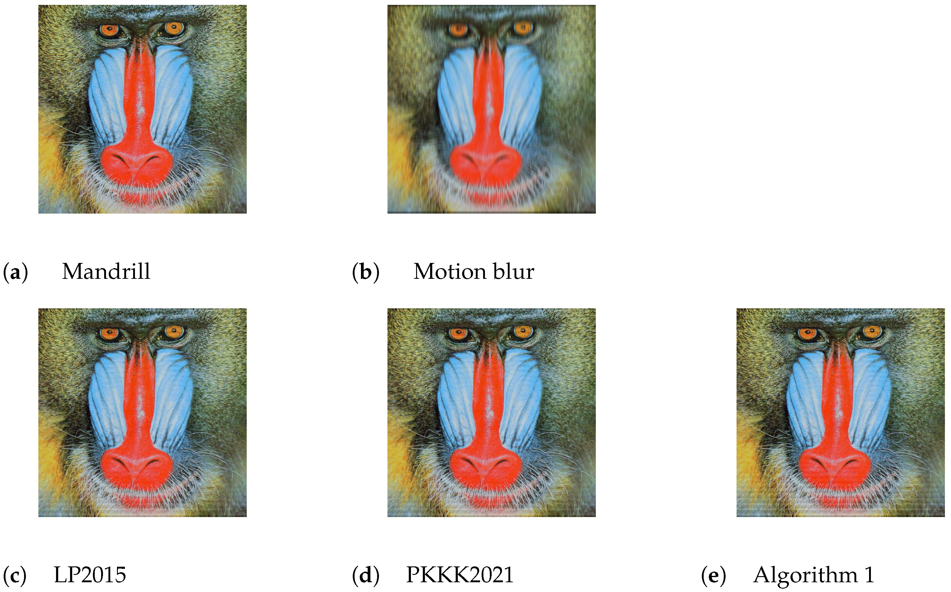
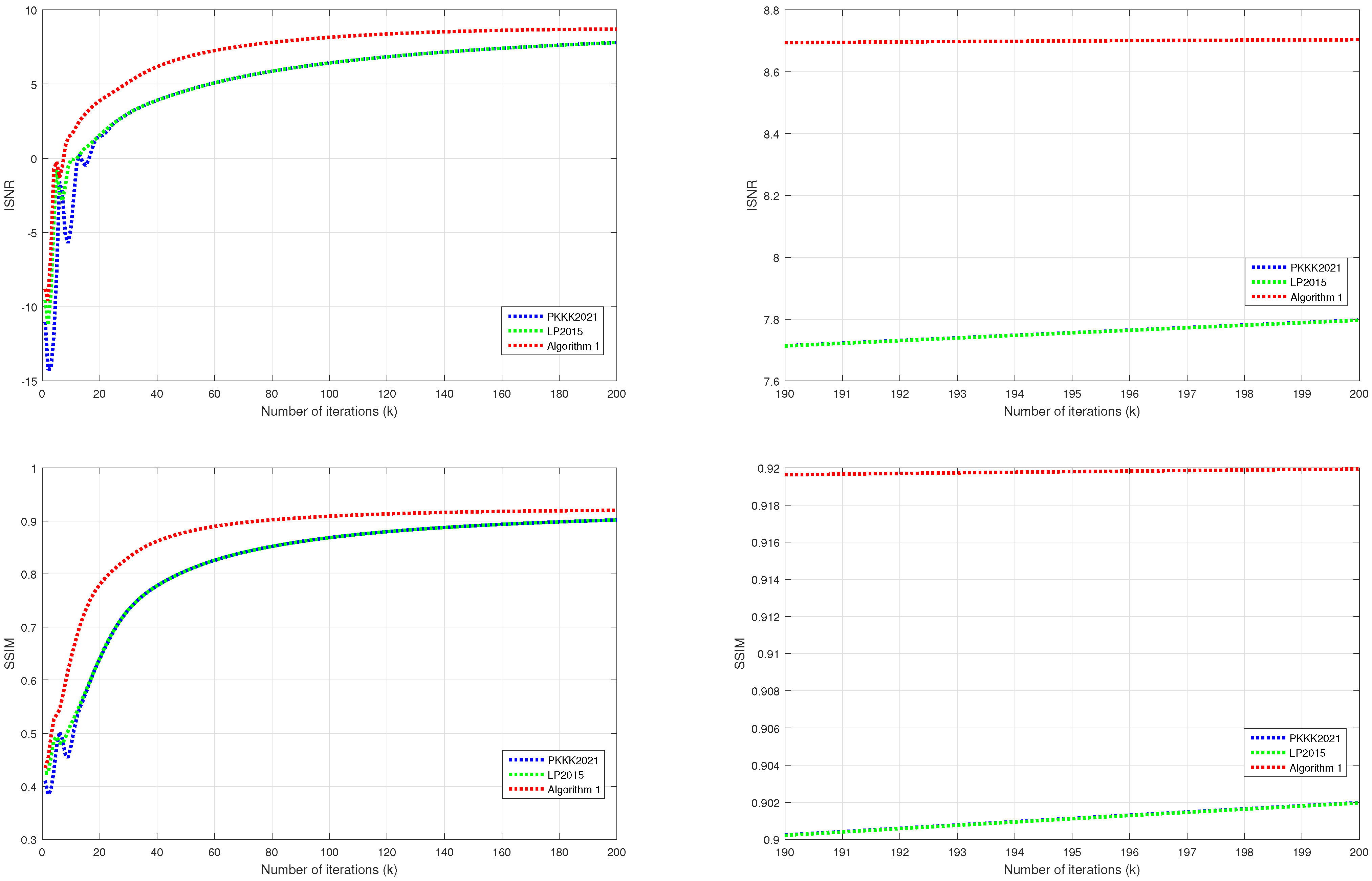
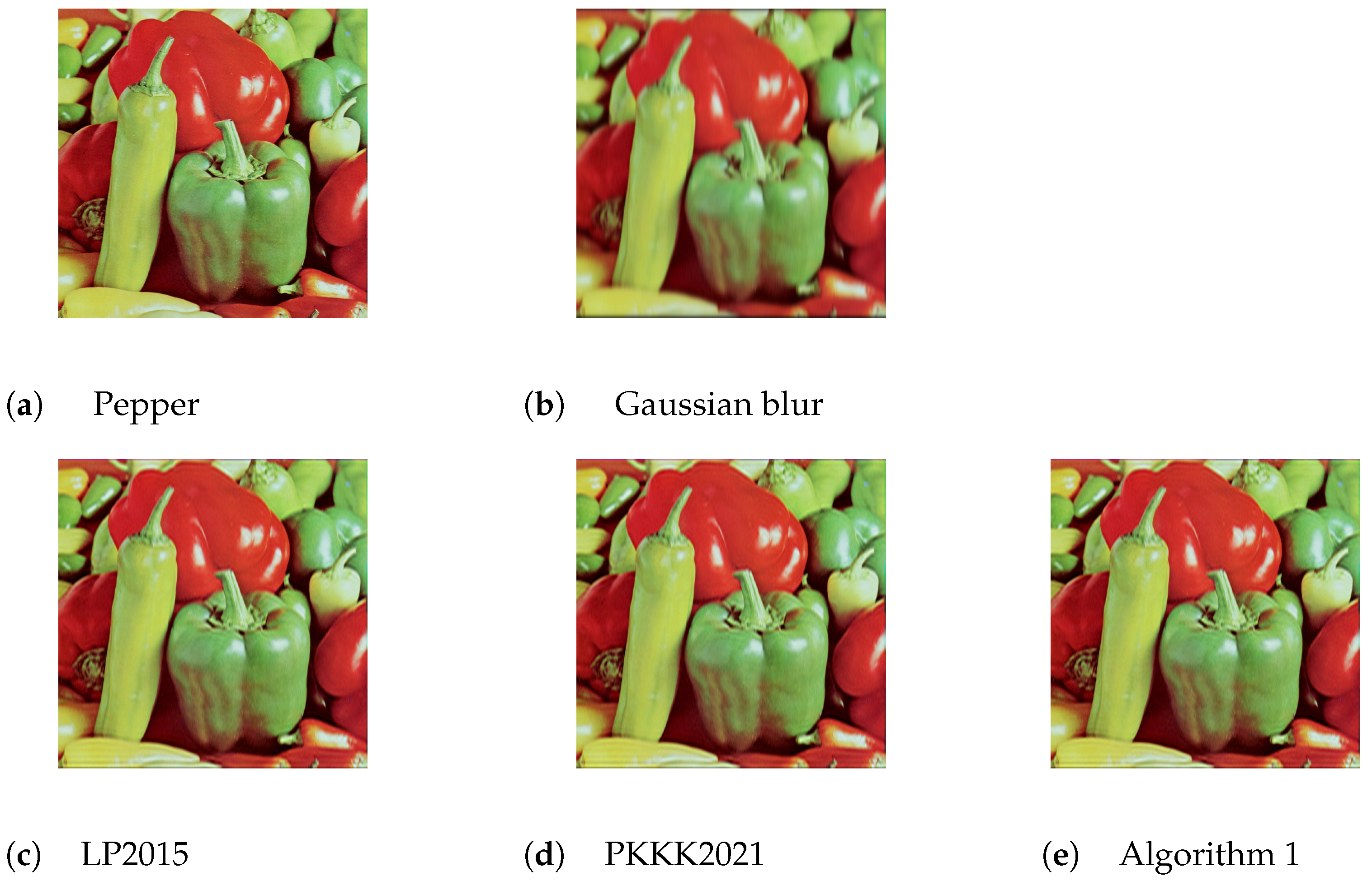
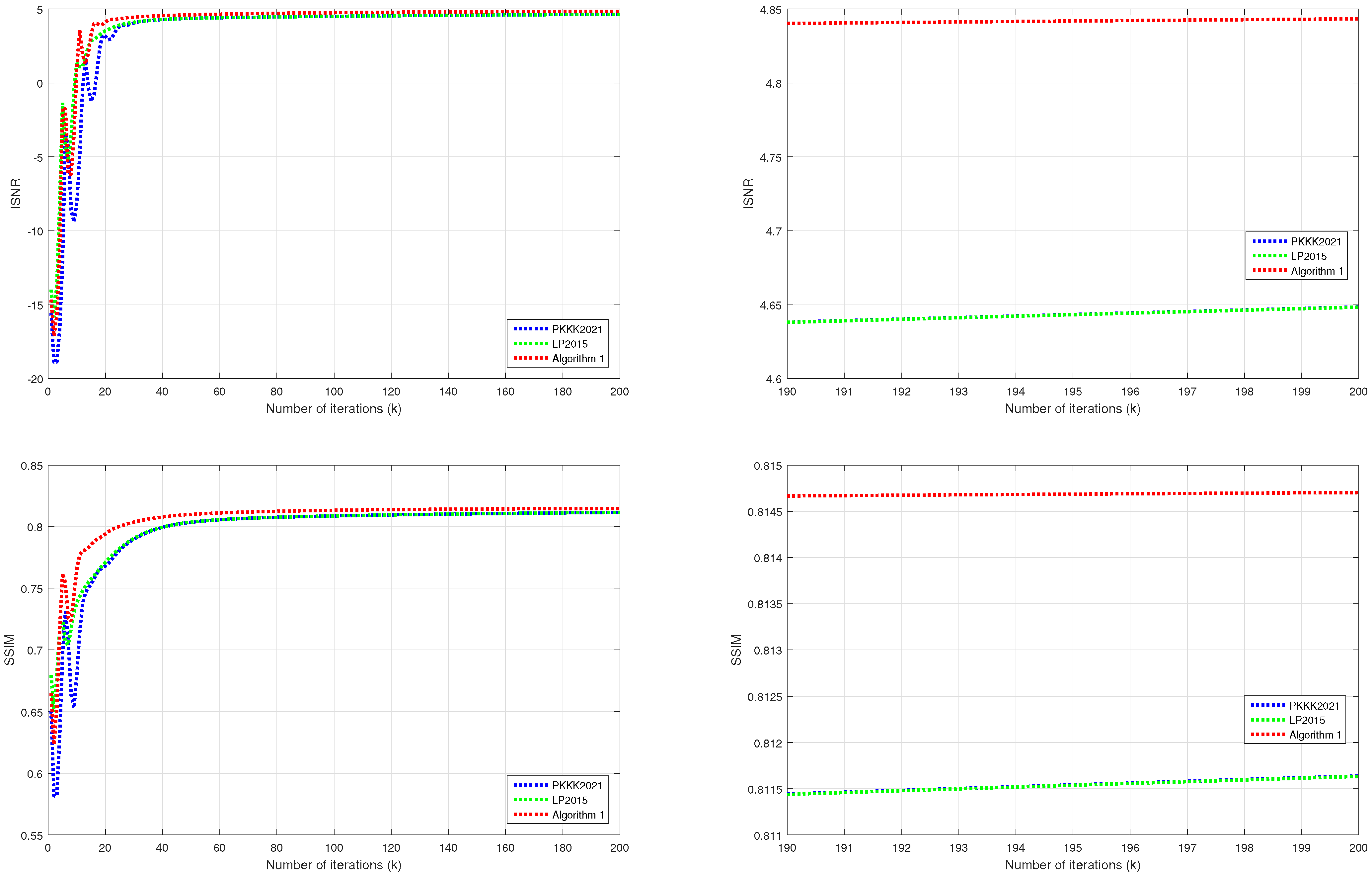
4. Applications to Image Deblurring Problems and Their Numerical Experiments

In this section, we aim to restore an image through the recommended algorithm, addressing tasks like image deblurring and denoising by using a degradation model that accurately represents real-world challenges in image restoration. Next, it is important to note that problem (1) can be seen as a particular problem of (13). With this in mind, we set up the following: C = E = f ( · ) , and D = F = g ( · ) . Here, f ( u ) = 1 2 Λ u v 2 2 , g ( u ) = τ u 1 , and τ = 0.001 . Given this setup, it follows that f ( u ) = Λ * ( Λ u v ) , where the transpose of Λ is denoted as Λ * . To start the problem-solving process, we begin by selecting images and applying various blurring techniques to them. To solve (1), we apply Algorithm 1 under the following condition: ϑ n = 0.9 , s n = 0.5 150 n 1000 n + 100 , r n = 0.7 150 n 1000 n + 100 (for motion blur) and r n = 0.9 1 1000 n + 100 (for Gaussian blur). We compare our proposed algorithm with the algorithm (LP2015) presented in [6], and the algorithm (PKKK2021) introduced by Padcharoen et al. [8]. For the LP2015, we select parameter values as follows: ϑ n = 0.9 , and s n = 0.5 150 n 1000 n + 100 . Concerning the PKKK2021, we select the following parameter values: ϑ n = 0.9 and s n = 0.5 150 n 1000 n + 100 . To evaluate the quality of the deblurred image, we measure it using the structural similarity index measure (SSIM) [38] and the improvement in the signal–to–noise ratio (ISNR) for images, which is defined as follows:
ISNR ( n ) = 10 log 10 u v 2 2 u u n 2 2 ,
where u, v and u n represent the original image, the degraded image, and the restored image at iteration n, respectively. The numerical results related to ISNR and SSIM are shown in the following Figure 1, Figure 2, Figure 3 and Figure 4.
Our algorithm has demonstrated exceptional performance in image deblurring, outperforming other algorithms, as supported by the experimental results in Table 1 and Table 2.

5. Conclusions

We invented and studied double Tseng’s algorithms with an inertial term consisting of two monotone operators, such as those in Algorithm 1. We successfully proved weak convergence under some mild conditions on an operator; that is, a Lipschitz monotone operator, which is weaker than an inverse strongly monotone operator, as shown in Theorem 1. We applied Algorithm 1 to solve the image deblurring problem (1). More importantly, we performed numerical experiments to measure the performance and revealed the advantages of Algorithm 1; that is, the improvement in signal–to–noise ratio (ISNR) and structural similarity index measure (SSIM) measurement compared with those of some other, similar algorithms. These results clearly indicate that our method has significant advantages over some of the previous algorithms, as demonstrated by its superior performance in the numerical experiments presented in Section 4.

Author Contributions

Conceptualization, P.T., V.B., N.P. and K.U.; methodology, P.T. and K.U.; software, P.T. and K.U.; validation, P.T., V.B., N.P. and K.U.; convergence analysis, P.T. and K.U.; investigation, P.T. and K.U.; writing—original draft preparation, P.T. and K.U.; writing—review and editing, P.T., V.B., N.P. and K.U.; visualization, P.T. and K.U.; project administration, P.T. and K.U. All authors have read and agreed to the published version of the manuscript.

Funding

K.U. is supported by Naresuan University (NU) and the National Science, Research and Innovation Fund (NSRF). Grant No. R2566B013.

Data Availability Statement

The original contributions presented in the study are included in the article, further inquiries can be directed to the corresponding author/s.

Acknowledgments

The authors express their gratitude to the editors and anonymous referees for their valuable comments and suggestions, which have contributed to the enhancement of the paper’s quality and presentation. The authors sincerely thank Vasile Berinde for the ERASMUS+ grant awarded to Purit Thammasiri for his three-month research visit at the Faculty of Sciences, Technical University of Cluj-Napoca, North University Centre of Baia Mare, Romania. Moreover, this work was supported by Naresuan University (NU), and National Science, Research and Innovation Fund (NSRF). Grant NO. R2566B013.

Conflicts of Interest

The authors declare that they have no conflicts of interest.

References

  1. Lions, P.L.; Mercier, B. Splitting Algorithms for the Sum of Two Nonlinear Operators. SIAM J. Numer. Anal. 1979, 16, 964–979. [Google Scholar] [CrossRef]
  2. Passty, G.B. Ergodic convergence to a zero of the sum of monotone operators in Hilbert space. J. Math Anal Appl. 1979, 72, 383–390. [Google Scholar] [CrossRef]
  3. Tseng, P. A Modified Forward-Backward Splitting Method for Maximal Monotone Mappings. SIAM J. Control. Optim. 2000, 38, 431–446. [Google Scholar] [CrossRef]
  4. Alvarez, F.; Attouch, H. An inertial proximal method for maximal monotone operators via discretization of a nonlinear oscillator with damping. Set Valued Anal. 2001, 9, 3–11. [Google Scholar] [CrossRef]
  5. Polyak, B.T. Some methods of speeding up the convergence of iterative methods. Zh. Vychisl. Mat. Mat. Fiz. 1964, 4, 1–17. [Google Scholar] [CrossRef]
  6. Lorenz, D.A.; Pock, T. An Inertial Forward-Backward Algorithm for Monotone Inclusions. J. Math. Imaging Vis. 2015, 51, 311–325. [Google Scholar] [CrossRef]
  7. Moudafi, A.; Oliny, M. Convergence of a splitting inertial proximal method for monotone operators. J. Comput. Appl. Math. 2003, 155, 447–454. [Google Scholar] [CrossRef]
  8. Padcharoen, A.; Kitkuan, D.; Kumam, W.; Kumam, P. Tseng methods with inertial for solving inclusion problems and application to image deblurring and image recovery problems. Comput. Math. Methods 2020, 3, e1088. [Google Scholar] [CrossRef]
  9. Berinde, V. Approximating Fixed Points of Lipschitzian Pseudocontractions. In Proceedings of the Mathematics & Mathematics Education, Bethlehem, Palestine, 9–12 August 2000; World Scientific Publishing: River Edge, NJ, USA, 2002. [Google Scholar]
  10. Berinde, V. Iterative Approximation of Fixed Points, 2nd ed.; Lecture Notes in Mathematics, 1912; Springer: Berlin/Heidelberg, Germany, 2007. [Google Scholar]
  11. Takahashi, W. Nonlinear Functional Analysis; Yokohama Publishers: Yokohama, Japan, 2000. [Google Scholar]
  12. Takahashi, W. Introduction to Nonlinear and Convex Analysis; Yokohama Publishers: Yokohama, Japan, 2009. [Google Scholar]
  13. Ungchittrakool, K. Existence and convergence of fixed points for a strict pseudo-contraction via an iterative shrinking projection technique. J. Nonlinear Convex Anal. 2014, 15, 693–710. [Google Scholar] [CrossRef]
  14. Inchan, I. Convergence theorem of a new iterative method for mixed equilibrium problems and variational inclusions: Approach to variational inequalities. Appl. Math. Sci. 2012, 6, 747–763. [Google Scholar]
  15. Adamu, A.; Kumam, P.; Kitkuan, D.; Padcharoen, A. Relaxed modified Tseng algorithm for solving variational inclusion problems in real Banach spaces with applications. Carpathian J. Math. 2023, 39, 1–26. [Google Scholar] [CrossRef]
  16. Ungchittrakool, K.; Plubtieng, S.; Artsawang, N.; Thammasiri, P. Modified Mann-type algorithm for two countable families of nonexpansive mappings and application to monotone inclusion and image restoration problems. Mathematics 2023, 11, 2927. [Google Scholar] [CrossRef]
  17. Artsawang, N.; Plubtieng, S.; Bagdasar, O.; Ungchittrakool, K.; Baiya, S.; Thammasiri, P. Inertial Krasnosel’skiĭ-Mann iterative algorithm with step-size parameters involving nonexpansive mappings with applications to solve image restoration problems. Carpathian J. Math. 2024, 40, 243–261. [Google Scholar] [CrossRef]
  18. Alvarez, F. Weak convergence of a relaxed and inertial hybrid projection-proximal point algorithm for maximal monotone operators in Hilbert space. SIAM J. Optim. 2004, 14, 773–782. [Google Scholar] [CrossRef]
  19. Artsawang, N.; Ungchittrakool, K. Inertial Mann-type algorithm for a nonexpansive mapping to solve monotone inclusion and image restoration problems. Symmetry 2020, 12, 750. [Google Scholar] [CrossRef]
  20. Attouch, H.; Bolte, J.; Svaiter, B.F. Convergence of descent methods for semi-algebraic and tame problems: Proximal algorithms, forward-backward splitting, and regularized Gauss-Seidel methods. Math. Program. 2009, 137, 91–129. [Google Scholar] [CrossRef]
  21. Baiya, S.; Plubtieng, S.; Ungchittrakool, K. An inertial shrinking projection algorithm for split equilibrium and fixed point problems in Hilbert spaces. J. Nonlinear Convex Anal. 2021, 22, 2679–2695. [Google Scholar]
  22. Baiya, S.; Ungchittrakool, K. Accelerated hybrid algorithms for nonexpansive mappings in Hilbert spaces. Nonlinear Funct. Anal. Appl. 2022, 27, 553–568. [Google Scholar] [CrossRef]
  23. Baiya, S.; Ungchittrakool, K. Modified inertial Mann’s algorithm and inertial hybrid algorithm for k-strict pseudo-contractive mappings. Carpathian J. Math. 2023, 39, 27–43. [Google Scholar] [CrossRef]
  24. Dong, Q.L.; Yuan, H.B.; Cho, Y.J.; Rassias, T.M. Modified inertial Mann algorithm and inertial CQ-algorithm for nonexpansive mappings. Optim. Lett. 2018, 12, 87–102. [Google Scholar] [CrossRef]
  25. Munkong, J.; Dinh, B.V.; Ungchittrakool, K. An inertial extragradient method for solving bilevel equilibrium problems. Carpathian J. Math. 2020, 36, 91–107. [Google Scholar] [CrossRef]
  26. Munkong, J.; Dinh, B.V.; Ungchittrakool, K. An inertial multi-step algorithm for solving equilibrium problems. J. Nonlinear Convex Anal. 2020, 21, 1981–1993. [Google Scholar]
  27. Nesterov, Y. A method for solving a convex programming problem with convergence rate O(1/K2). Dokl. Math. 1983, 27, 367–372. [Google Scholar]
  28. Yuying, T.; Plubtieng, S.; Inchan, I. Inertial hybrid and shrinking projection methods for sums of three monotone operators. J. Comput. Anal. Appl. 2024, 32, 85–94. [Google Scholar]
  29. Byrne, C. A unified treatment of some iterative algorithms in signal processing and image reconstruction. Inverse Probl. 2004, 20, 103–120. [Google Scholar] [CrossRef]
  30. Combettes, P.L. Constrained image recovery in a product space. In Proceedings of the IEEE International Conference on Image Processing, Washington, DC, USA, 23–26 October 1995; IEEE Computer Society Press: Los Alamitos, CA, USA, 1995; pp. 2025–2028. [Google Scholar]
  31. Kitkuan, D.; Kumam, P.; Martínez-Moreno, J.; Sitthithakerngkiet, K. Inertial viscosity forward–backward splitting algorithm for monotone inclusions and its application to image restoration problems. Int. J. Comput. Math. 2019, 97, 482–497. [Google Scholar] [CrossRef]
  32. Podilchuk, C.I.; Mammone, R.J. Image recovery by convex projections using a least-squares constraint. J. Opt. Soc. Am. 1990, 7, 517–521. [Google Scholar] [CrossRef]
  33. Artsawang, N. Accelerated preconditioning Krasnosel’skiĭ-Mann method for efficiently solving monotone inclusion problems. AIMS Math. 2023, 8, 28398–28412. [Google Scholar] [CrossRef]
  34. Brézis, H.; Chapitre, I.I. Operateurs maximaux monotones. North Holl. Math Stud. 1973, 5, 19–51. [Google Scholar]
  35. Bauschke, H.H.; Combettes, P.L. Convex Analysis and Monotone Operator Theory in Hilbert Spaces; CMS Books in Mathematics; Springer: New York, NY, USA, 2011. [Google Scholar]
  36. Opial, Z. Weak convergence of the sequence of successive approximations for nonexpansive mappings. Bull. Am. Math. Soc. 1967, 73, 591–597. [Google Scholar] [CrossRef]
  37. Thammasiri, P.; Wangkeeree, R.; Ungchittrakool, K. A modified inertial Tseng’s algorithm with adaptive parameters for solving monotone inclusion problems with efficient applications to image deblurring problems. J. Comput. Anal. Appl. 2024; in press. [Google Scholar]
  38. Wang, Z.; Bovik, A.C.; Sheikh, H.R.; Simoncelli, E.P. Image quality assessment: From error visibility to structural similarity. IEEE Trans. Image Process. 2004, 13, 600–612. [Google Scholar] [CrossRef] [PubMed]
Figure 1. (a) displays the original image, which is named ‘Mandrill’, while (b) presents the images degraded by motion blur and (ce) describe the deblurred images obtained using LP2015 [6], PKKK2021 [8], and Algorithm 1, respectively.
Mathematics 12 03138 g001
Figure 2. The figures demonstrate the performance of deblurring using three algorithms. We used the improvement in signal–to–noise ratio (ISNR) and structural similarity index measure (SSIM) as tools to compare the deblurring performance of the ‘Mandrill’ image.
Mathematics 12 03138 g002
Figure 3. (a) displays the original image ‘Pepper’, while (b) presents the images degraded by Gaussian blur and (ce) describe the deblurred images obtained using LP2015 [6], PKKK2021 [8], and Algorithm 1, respectively.
Mathematics 12 03138 g003
Figure 4. The figures demonstrate the performance of deblurring using three algorithms. We used the improvement in signal–to–noise ratio (ISNR) and structural similarity index measure (SSIM) as tools to compare the deblurring performance of the ‘Pepper’ image.
Mathematics 12 03138 g004
Table 1. In this table, we present the values of the improvement in signal–to–noise ratio (ISNR) and structural similarity index measure (SSIM) for each algorithm to demonstrate the behavior of the deblurring of the ‘Mandrill’ image.
(n)ISNRSSIM
Algorithm 1PKKK2021LP2015Algorithm 1PKKK2021LP2015
1−8.8946−11.0381−9.56120.43440.41070.4249
101.6975−4.6297−0.06110.64990.47630.5172
506.93354.55254.55350.88170.80570.8058
1008.21976.42236.42260.91020.86850.8685
2008.70977.79677.79610.92010.90190.9019
Table 2. In this table, we present the values of the improvement in signal–to–noise ratio (ISNR) and structural similarity index measure (SSIM) for each algorithm to demonstrate the behavior of the deblurring of the ‘Pepper’ image.
(n)ISNRSSIM
Algorithm 1PKKK2021LP2015Algorithm 1PKKK2021LP2015
1−14.6677−15.5479−13.98920.66490.65090.6796
101.0734−8.08661.34290.76580.67960.7384
504.61214.37194.37310.81000.80360.8037
1004.75624.51134.51150.81330.80870.8088
2004.84344.64844.64830.81470.81160.8116
Disclaimer/Publisher’s Note: The statements, opinions and data contained in all publications are solely those of the individual author(s) and contributor(s) and not of MDPI and/or the editor(s). MDPI and/or the editor(s) disclaim responsibility for any injury to people or property resulting from any ideas, methods, instructions or products referred to in the content.

