Article

Iterative Dissipativity of Partial Difference Equation Dynamics in Open-Loop Iterative Learning Control Mode

by
Tengfei Xiao
School of Intelligent Systems Engineering, Sun Yat-sen University, Shenzhen 518107, China
Mathematics 2024, 12(19), 3128; https://doi.org/10.3390/math12193128
Submission received: 2 September 2024 / Revised: 3 October 2024 / Accepted: 4 October 2024 / Published: 6 October 2024
(This article belongs to the Section C2: Dynamical Systems)

Abstract

:
Complex physical processes, which could evolve in both spatial and temporal dimensions and be represented by partial difference equations, could also operate in a repetitive mode with iterative learning methods as suitable control laws. For these three-dimensional systems (of the spatial, temporal, and iterative dimensions), the stability in the iterative direction is critical for many applications, which can be analyzed and synthesized under the proposed concept of iterative dissipativity. The definition of iterative dissipativity, which is first introduced in this paper, encapsulates the dominant information in both the spatial and temporal dimensions, while also placing a particular emphasis on the iteration improvement. This property allows for the derivation of sufficient conditions for asymptotic stability in the iteration direction, which are represented by linear matrix inequality criteria that can be readily solved. Performance in both the spatial and temporal dimensions can also be satisfied under this iterative dissipativity concept, even in absence of real-time feedback. Moreover, the optimization solutions of the control parameters can be determined. Finally, a thermal process and a numeric example are presented to illustrate the effectiveness of the proposed iteratively dissipative learning control approach.

1. Introduction

In real-world applications, physical systems exhibit complex spatio-temporal dynamics [1,2,3,4,5] that can be represented by partial difference equations. For instance, thermal distribution dynamics in chemical engineering and flexible robotic link dynamics in aerospace engineering are two examples of such systems. These systems evolve in two dimensions, meaning that their states, inputs, and outputs depend on two independent variables (e.g., time and space). Two-dimensional system models, such as the Roesser model [6], which is a partial difference equation, are suitable for describing their dynamics. Furthermore, these systems could also operate in a repetitive mode, such as a thermal process required to heat or cool in a finite duration repetitively for some chemical reactions [7], or a flexible link rerunning an action [5]. In order to describe the iterative repetitiveness of such systems, an iteration dimension should be added to the system models. Overall, these systems should be treated as three-dimensional (3-D) models, incorporating two-dimensional Roesser dynamics and a special iterative structure.
For such systems, the stability in the iteration direction is a prominent feature in applications where the iterative learning control (ILC) approach [8,9,10,11,12], which enhances the stability performance through learning iteratively, is found to be a promising strategy. The existing literature on ILC for one-dimensional lumped parameter systems of temporal dynamics has been extensive, yet the ILC designs that account for the special properties of the spatio-temporal dynamics remain limited. Among these, the works in [13,14] had employed multi-dimensional system theory to analyze spatio-temporal dynamics, which were controlled by ILC schemes. In these control designs, ILC with some kinds of real-time feedback, as a closed-loop ILC, was exploited in order to achieve an acceptable performance along the trial. It was argued in these studies that undesirable behavior, such as exponential growth of the signals in the spatial and temporal directions, may be observed in the real applications. The integration of real-time feedback into ILC designs has the potential to enhance closed-loop stability, thereby preventing such undesirable performances along the trial. However, as the operational time is finite in these system configurations, a carefully selected initial iteration control input and a delicately designed iteration step-size already have the ability to effectively prevent trial performance from becoming too severely deviated. Real-time feedback, which is a complex factor in the control design and imposes real-time restrictions, is not always a necessity. Open-loop ILC, which employs only the errors observed in the last trial, is relatively simple and sufficient for the iterative convergence with satisfactory trial performances. The challenge lies in the design of the open-loop ILC.
Some attempts have been made to investigate the open-loop ILC of spatio-temporal dynamics. For example, ref. [15] established a P-type learning control law for a discrete distributed parameter system with the help of the discrete Green formula and the analogous discrete Gronwall inequality. Additionally, a PID-type ILC was designed for the Roesser model in [16]. The sufficient conditions for convergence in these two papers both require that the systems have a zero relative degree. For systems with a non-zero relative degree, ref. [17] proposed a two-gain ILC law with sufficient conditions of iterative stability for a special kind of Roesser model. However, in the aforementioned references, nonlinear inequalities of control parameters, which may depend on the eigenvalues of some system matrices, are employed as tests for the feasibility of the algorithms. Verification of these non-linear criteria is computationally challenging, impeding the analysis and synthesis of 3-D systems in an iterative repetitive mode.
The design of the open-loop ILC can be facilitated by a analogous dissipative systems theory. In this paper, we would propose an iterative dissipative concept for the design, with simple linear matrix inequality (LMI) conditions serving as the design criteria. The notion of dissipative systems, which was firstly introduced in [18], is a generalization of systems dissipating energy in an abstract sense. It has been applied to the stability analysis of linear [19] and non-linear one-dimensional systems [20]. Based on the theory of dissipative systems, quadratic dissipative control was proposed by [21] for one-dimensional linear discrete-time systems to achieve asymptotic stability and strict quadratic dissipativity. The theory of dissipative systems was extended to two-dimensional systems in [22]. In that work, two-dimensional dissipativity was defined, and the problems of two-dimensional dissipative control and filtering for a linear discrete-time Roesser model were investigated. The developments of two-dimensional dissipative control laws can be used for the ILC designs of one-dimensional systems of temporal dynamics [23,24,25], although a non-linear real-time feedback compensatory term is required for the exponential stability in these designs. Two-dimensional methods can be extended directly to solve the 3-D problem by reducing the 3-D structure into a two-dimensional one with the help of the lifting technique [26]. The main idea of the lifting technique is to discretize the states in the spatial dimension into vectors of points. However, this will result in a vector dimension that is proportional to the point number in the spatial direction, which is usually too large for computation [14,27]. Thus, a 3-D dissipative concept should be considered to capture the dynamical evolution of the two-dimensional process, while simultaneously paying special attention to the iteration improvement. This basic idea in our work is based mainly on the one-dimensional Q-S-R- α dissipativity [21] and two-dimensional Q-S-R- α dissipativity [22] theories. Since these methods cannot efficiently deal with the 3-D iterative problems, we extend these ideas to the 3-D version. The 3-D version introduces an iterative scheme to the conventional Q-S-R- α dissipative concept, which provides more consideration of the iterative properties of the controlled system. Compared with other methods based on the “lifting technique”, the dimension of the test matrix in our scheme is extremely small, which provides computational efficiency for the control design.
The primary theoretical contribution of this work is the proposal of a novel 3-D iterative dissipative concept that serves as a mediator for the straightforward design of the open-loop ILC for the partial difference equation dynamics. The first benefit of the proposed iterative dissipativity concept is that the point-wise asymptotic convergence of the tracking error in the iteration direction can be proved, as the iterative convergence is a central focus of this work. Furthermore, the iterative dissipativity implies that the iterative convergence is monotonic. The controlled system would not deteriorate from trial to trial. Consequently the system can exhibit stable behavior along the trial in each iteration if the initial iteration control is selected appropriately. The second benefit of the concept is that it entails a stability criterion which is an LMI of the controller parameters with a testing matrix of a small dimension. The LMI is computationally simple with the help of the sophisticated software packages [28,29], making it possible to test the feasibility of the controller parameters in an efficient manner. Thirdly, iterative dissipativity represents a generalization of some iterative performances, such as the iterative convergence speed of the controller. The analysis of iterative dissipativity allows us to address the optimal iterative convergence speed. Generally speaking, we propose a special 3-D dissipativity theory with a focus on the iterative direction, based on which the open-loop linear ILC can be designed while its feasibility and optimality can be easily tested.
The structure of this paper is as follows. In Section 2, the iterative dissipativity of Q-S-R- α type is defined for iteratively repetitive 3-D systems with sufficient LMI conditions. In Section 3, the iteratively asymptotic stability is derived as a result of iterative dissipativity, while the feasibility and optimization of the control parameters are solved with relative ease. Section 4 provides a thermal process and a numeric example to illustrate the effectiveness of the proposed scheme. Finally, Section 5 provides a summary of this paper.

2. Iterative Dissipativity of 3-D Systems

The evolution of a 3-D system considered in this paper, such as a repetitive thermal process [7,30] or a re-running flexible link [5], can be considered to follow three directions: spatial, temporal, and iterative. For each iteration, the spatio-temporal dynamics can be described by a partial difference equation, such as the Roesser model [6] considered in this paper. Thus, the following 3-D discrete linear model in an iteratively repetitive mode is used as the system under consideration.
x k h ( i + 1 , j ) = A 11 x k h ( i , j ) + A 12 x k v ( i , j ) + B 1 u k ( i , j ) x k v ( i , j + 1 ) = A 21 x k h ( i , j ) + A 22 x k v ( i , j ) + B 2 u k ( i , j ) y k ( i , j ) = C 1 x k h ( i , j ) + C 2 x k v ( i , j ) + D u k ( i , j )
where x k h ( i , j ) R m and x k v ( i , j ) R n are the horizontal (the spatial variable i { 0 , 1 , 2 , T i } ) and the vertical (the temporal variable j { 0 , 1 , 2 , T j } ) states, respectively; k { 0 , 1 , 2 , } is the iteration number; u k ( i , j ) R p is the input; and y k ( i , j ) R q is the system output. A 11 , A 12 , A 21 , A 22 , B 1 , B 2 , C 1 , C 2 , and D are the system matrices with appropriate dimensions. The notation can be condensed in the following compact forms:
x k ( i , j ) x k h ( i , j ) x k v ( i , j ) T , x ¯ k ( i , j ) x k h ( i + 1 , j ) x k v ( i , j + 1 ) T , A A 11 A 12 A 21 A 22 , B B 1 B 2   and C C 1 C 2 .
The Roesser model is now written as
x ¯ k ( i , j ) = A x k ( i , j ) + B u k ( i , j ) ,
y k ( i , j ) = C x k ( i , j ) + D u k ( i , j ) .
The control law for this repetitive 3-D system is iteratively updated as follows:
u k + 1 ( i , j ) = u k ( i , j ) + Δ u k ( i , j )
where Δ u k ( i , j ) is the updating part of the iterative learning control law. Conveniently, we can set u 0 ( i , j ) , the control signal in the first iteration, to zero. Then, the updating law will produce the control signal for all iterations. In this paper, we consider an open-loop iterative learning control law whose updating part is of the following general spatio-temporal form:
Δ u k ( i , j ) = L x k ( i , j ) + K x ¯ k ( i , j )
where L and K are control parameter matrices with appropriate dimensions.
Remark 1.
When we select K = 0 in the control law (6), the controller is of a spatio-temporal proportional type. When we select L = K , the controller is in the form of a spatio-temporal derivative type.
To facilitate stability analysis, zero boundary conditions are enforced on the system.
Assumption 1.
The iteratively repetitive 3-D system (3) and (4) is under zero boundary conditions, such that
x k h ( i , 0 ) = x k v ( i , 0 ) = 0 f o r   a l l   i   a n d   k ,
x k h ( 0 , j ) = x k v ( 0 , j ) = 0 f o r   a l l   j   a n d   k .
We now propose the iterative dissipativity of 3-D systems, which is the fundamental concept for our analysis.
Definition 1.
The system (3) and (4) is iteratively dissipative if there exists a input energy function  V k i = 0 T i j = 0 T j V ( x k ( i , j ) , u k ( i , j ) , y k ( i , j ) ) and a system energy function W k i = 0 T i j = 0 T j W ( u k ( i , j ) , y k ( i , j ) ) , such that
V k V k + 1 W k .
Overall, iterative dissipativity implies that the input energy decreases as the iteration proceeds and that the decrease is greater than a fraction of the system energy. It provides more consideration of the iterative properties of the controlled system. As a special case of iterative dissipativity, we define the Q-S-R- α iterative dissipativity for the specific analysis of the systems. The Q-S-R- α dissipative concept is based on one-dimensional Q-S-R- α dissipativity [21] and two-dimensional Q-S-R- α dissipativity [22] theories. We extend the ideas to the 3-D version with an iterative scheme.
Definition 2.
Given a matrix S and two positive semi-definite matrices Q and R, the iteratively repetitive 3-D system (3) and (4) is Q-S-R-α iteratively dissipative if there exists a positive number α, such that the system is iteratively dissipative with the input energy function
V k = 1 α i = 0 T i j = 0 T j u k T ( i , j ) u k ( i , j )
and the system energy function
W k = i = 0 T i j = 0 T j y k T ( i , j ) Q y k ( i , j ) + y k T ( i , j ) S u k ( i , j ) + u k T ( i , j ) R u k ( i , j ) .
In this formulation, the input energy is defined as a quadratic function of the input variables. The definition of system energy can take into account a variety of conditions. For example, if Q = I , S = R = 0 , then the system energy represents the output energy; if Q = S = 0 , R = I , then the system energy represents the input energy; and if Q = ( C 1 ) T C 1 , S = 2 ( C 1 ) T C 1 D , R = ( C 1 D ) T C 1 D , then the system energy represents the state energy. It has different physical interpretations. In particular, we show in Remark 6 that when the system energy represents the input energy, Q-S-R- α iterative dissipativity can be interpreted as a kind of fast convergence speed. For the system configuration considered, the sufficient condition of the Q-S-R- α iterative dissipativity is obtained as an LMI criterion.
Theorem 1.
Given Q, S, and R, the 3-D system (3) and (4) with the learning control laws (5) and (6) and Assumption 1 is Q-S-R-α iteratively dissipative if there exist L, K, and α, and P = P h 0 0 P v , where P h R m × m and P v R n × n are positive definite matrices such that the following LMI condition is satisfied:
Ω = Ω 11 Ω 12 Ω 13 * Ω 22 Ω 23 * * Ω 33 < 0
where
Ω 11 = A T P A P + α C T Q C Ω 22 = B T P B + α D T Q D + α 2 D T S + α 2 S T D + α R + K B + B T K T Ω 33 = I Ω 12 = A T P B + α C T Q D + α 2 C T S + L T + A T K T Ω 13 = L T + A T K T Ω 23 = B T K T
and * is an ellipsis for terms that are induced by symmetry.
Proof. 
As Ω < 0 , the Schur complement of Ω 33 in Ω is
Γ = Ω 11 + Ω 13 Ω 13 T Ω 12 + Ω 13 Ω 23 T * Ω 22 + Ω 23 Ω 23 T < 0 .
Thus,
x k T ( i , j ) u k T ( i , j ) Γ x k ( i , j ) u k ( i , j ) 0 ,
that is,
( A x k ( i , j ) + B u k ( i , j ) ) T P ( A x k ( i , j ) + B u k ( i , j ) ) x k T ( i , j ) P x k T ( i , j ) + α C x k ( i , j ) + D u k ( i , j ) T Q C x k ( i , j ) + D u k ( i , j ) + α C x k ( i , j ) + D u k ( i , j ) T S u k ( i , j ) + α u k T ( i , j ) R u k ( i , j ) + [ ( L + K A ) x k ( i , j ) + ( 2 I + K B ) u k ( i , j ) ] T ( L + K A ) x k ( i , j ) + K B u k ( i , j ) 0 .
From (3), (5), and (6), we have
u k + 1 T ( i , j ) u k + 1 ( i , j ) u k T ( i , j ) u k ( i , j ) = ( u k + 1 ( i , j ) + u k ( i , j ) ) T ( u k + 1 ( i , j ) u k ( i , j ) ) = ( u k ( i , j ) + L x k ( i , j ) + K x ¯ k ( i , j ) + u k ( i , j ) ) T ( u k ( i , j ) + L x k ( i , j ) + K x ¯ k ( i , j ) u k ( i , j ) ) = ( 2 u k ( i , j ) + L x k ( i , j ) + K ( A x k ( i , j ) + B u k ( i , j ) ) ) T ( L x k ( i , j ) + K ( A x k ( i , j ) + B u k ( i , j ) ) ) = ( L + K A ) x k ( i , j ) + ( 2 I + K B ) u k ( i , j ) T ( L + K A ) x k ( i , j ) + K B u k ( i , j ) .
By introducing (3), (4), and the above Equation (15) into (14), we have
x ¯ k T ( i , j ) P x ¯ k ( i , j ) x k T ( i , j ) P x k T ( i , j ) + α y k T ( i , j ) Q y k ( i , j ) + α y k T ( i , j ) S u k ( i , j ) + α u k T ( i , j ) R u k ( i , j ) + u k + 1 T ( i , j ) u k + 1 ( i , j ) u k T ( i , j ) u k ( i , j ) 0 .
which leads to
i = 0 T i j = 0 T j x ¯ k T ( i , j ) P x ¯ k ( i , j ) i = 0 T i j = 0 T j x k T ( i , j ) P x k T ( i , j ) + α i = 0 T i j = 0 T j ( y k T ( i , j ) Q y k ( i , j ) + y k T ( i , j ) S u k ( i , j ) + u k T ( i , j ) R u k ( i , j ) ) + i = 0 T i j = 0 T j u k + 1 T ( i , j ) u k + 1 ( i , j ) u k T ( i , j ) u k ( i , j ) 0 .
With a zero boundary condition, as follows:
i = 0 T i j = 0 T j x ¯ k T ( i , j ) P x ¯ k ( i , j ) i = 0 T i j = 0 T j x k T ( i , j ) P x k T ( i , j ) = x k h T ( T i + 1 , T j ) P h x k h ( T i + 1 , T j ) + x k v T ( T i , T j + 1 ) P h x k v ( T i , T j + 1 ) 0 .
As a result, we have
α i = 0 T i j = 0 T j ( y k T ( i , j ) Q y k ( i , j ) + y k T ( i , j ) S u k ( i , j ) + u k T ( i , j ) R u k ( i , j ) ) + i = 0 T i j = 0 T j u k + 1 T ( i , j ) u k + 1 ( i , j ) u k T ( i , j ) u k ( i , j ) 0
which implies that the system is Q-S-R- α iteratively dissipative. □
Compared to other Q-S-R- α dissipative theorems, Theorem 1 provides a result on the iteration direction. What this means is that if we can find unknown variables L, K, α , and P such that LMI (10) is satisfied, then the system can have an iterative dissipative property, which is defined in Definitions 1 and 2. This property is shown to be important for the iterative convergence discussed in Section 3. We also have the following remarks on the theorem.
Remark 2.
Inequality (10) is an LMI with L, K, α, and P as variables. This can be proved by decomposing and rearranging the elements of the matrix.
Remark 3.
The positive number α can be interpreted as a design parameter representing the strictness of the iterative dissipativity in Definition 1. As the value of α is increased, the iterative dissipativity is enhanced. However, it should be noted that an increased value of α may render the LMI criterion (10) challenging to fulfill. The maximum value of α can be regarded as the optimal iterative dissipativity performance bound α * .
Remark 4.
The control parameters L and K are feasible if the LMI criterion (10) is met. Furthermore, the optimal iterative dissipativity parameters L and K are obtained if the performance bound α * is achieved. Thus, the feasibility and optimization of the control parameters are transformed to the LMI problems, which can be readily solved with existing LMI software packages [28,29].
It is required that A T P A P < 0 in the condition (10), which implies that the system is asymptotically stable in the i and j dimensions under zero input, according to a theorem provided in [31]. In fact, even in the absence of asymptotic stability in the i and j dimensions, the iterative dissipativity of the system can still be guaranteed by the following theorem, provided that the matrix B is non-singular. In the following theorem, F = B 1 denotes the inverse of B, and s y m { G } indicates G + G T .
Theorem 2.
Given Q, S, and R, the 3-D system (3) and (4) with the learning control laws (5) and (6) and Assumption 1 is Q-S-R-α iteratively dissipative if B is non-singular and there exist L, K, and α such that the following LMI condition is satisfied:
Ω = Ω 11 Ω 12 Ω 13 * Ω 22 Ω 23 * * Ω 33 < 0
where
Ω 11 = α ( D F ) T Q D F + s y m { α 2 ( D F ) T S F } + α F T R F + s y m { F T K } Ω 22 = α ( C D F A ) T Q ( C D F A ) s y m { α 2 ( C D F A ) T S F A } + α ( F A ) T R F A s y m { ( F A ) T L } Ω 33 = I Ω 12 = α ( D F ) T Q ( C D F A ) α 2 ( D F ) T S F A + α 2 ( C D F A ) T S F α F T R F A + F T L K T F A Ω 13 = K T Ω 23 = L T
and * is an ellipsis for terms that are induced by symmetry.
Proof. 
As Ω < 0 , the Schur complement of Ω 33 in Ω is
Γ = Ω 11 + Ω 13 Ω 13 T Ω 12 + Ω 13 Ω 23 T * Ω 22 + Ω 23 Ω 23 T < 0 .
Thus, we have
x ¯ k T ( i , j ) x k T ( i , j ) Γ x ¯ k ( i , j ) x k ( i , j ) 0 ,
that is,
α D F x ¯ k ( i , j ) + ( C D F A ) x k ( i , j ) T Q D F x ¯ k ( i , j ) + ( C D F A ) x k ( i , j ) + α D F x ¯ k ( i , j ) + ( C D F A ) x k ( i , j ) T S F x ¯ k ( i , j ) F A x k ( i , j ) + α F x ¯ k ( i , j ) F A x k ( i , j ) T R F x ¯ k ( i , j ) F A x k ( i , j ) + [ ( 2 F + K ) x ¯ k ( i , j ) ( 2 F A L ) x k ( i , j ) ] T K x ¯ k ( i , j ) + L x k ( i , j ) 0 .
Noting that
u k ( i , j ) = F x ¯ k ( i , j ) F A x k ( i , j ) ,
y k ( i , j ) = D F x ¯ k ( i , j ) + ( C D F A ) x k ( i , j )
and
u k + 1 T u k + 1 u k T ( i , j ) u k ( i , j ) = [ ( 2 F + K ) x ¯ k ( i , j ) ( 2 F A L ) x k ( i , j ) ] T K x ¯ k ( i , j ) + L x k ( i , j ) ,
we have
α y k T ( i , j ) Q y k ( i , j ) + α y k T ( i , j ) S u k ( i , j ) + α u k T ( i , j ) R u k ( i , j ) + u k + 1 T ( i , j ) u k + 1 ( i , j ) u k T ( i , j ) u k ( i , j ) 0 ,
leading to
α i = 0 T i j = 0 T j ( y k T ( i , j ) Q y k ( i , j ) + y k T ( i , j ) S u k ( i , j ) + u k T ( i , j ) R u k ( i , j ) ) + i = 0 T i j = 0 T j u k + 1 T ( i , j ) u k + 1 ( i , j ) u k T ( i , j ) u k ( i , j ) 0 .
This implies that the system is Q-S-R- α iteratively dissipative. □

3. Iterative Convergence Analysis of 3-D Systems

The iterative dissipativity implies the iterative stability of the systems. First, we give the definition of iterative stability.
Definition 3.
The 3-D system (3)–(6) is asymptotically stable point-wise in the iteration direction if the state, the input, and the output of the system approach 0 as the iteration number k goes to infinity for all i and j.
Then, the following theorem guarantees the asymptotic stability in the iteration direction, which is the prominent concern in the ILC applications.
Theorem 3.
The 3-D system (3)–(6) is asymptotically stable point-wise in the iteration direction if it is Q-S-R-α iteratively dissipative and one of the following conditions is satisfied:
1. 
Q 1 2 S * R > 0 ;
2. 
R > 0 , Q = S = 0 .
Proof. 
If one of the above conditions is satisfied, we have W k > 0 when there exist i and j such that u k ( i , j ) 0 . And because the 3-D system (3) and (4) is Q-S-R- α iteratively dissipative, we have
i = 0 T i j = 0 T j u k + 1 T ( i , j ) u k + 1 ( i , j ) i = 0 T i j = 0 T j u k T ( i , j ) u k ( i , j ) < 0 .
Note that the solution of (3) with a zero boundary condition can be expressed as
x k ( i , j ) = f = 0 i g = 0 j ϕ i j u k ( f , g )
where ϕ i j is some appropriate matrix.
If U k = [ u k T ( 0 , 0 ) u k T ( 0 , 1 ) u k T ( 1 , 0 ) u k T ( T 1 , T 2 ) ] T is defined and (3), (5), (6), and (31) are used, we obtain
U k + 1 = φ U k
where φ is some appropriate matrix.
Then, by defining the Lyapnov function as
Ψ k = i = 0 T i j = 0 T j u k T ( i , j ) u k ( i , j )
and utilizing (30), we have U k = 0 , which asymptotically stable according to the Lyapunov theory for discrete time systems. Thus, x k ( i , j ) , u k ( i , j ) and y k ( i , j ) approach 0 as k goes to infinity for all i and j. □
Remark 5.
Under the conditions of iterative dissipativity and iterative convergence, the so-called system energy W k is always positive. Then, the iterative dissipative property implies that the input energy V k declines monotonically as the iteration k increases. As a result, if a control is selected in the initial iteration with bounded signals and an acceptable level of performance, the system will remain bounded and the controlled performance will not degrade from trial to trial. This ensures that the system behaves well along the trial in any iteration, regardless of the absence of real-time feedback.
Remark 6.
The system energy function W k can take different values of Q, S, and R, which have different physical interpretations for a specific system and may be used to analyze different iterative attributes. For a general system, if Q = 0 , S = 0 , and R = I are chosen, we have
i = 0 T i j = 0 T j u k T ( i , j ) u k ( i , j ) i = 0 T i j = 0 T j u k + 1 T ( i , j ) u k + 1 ( i , j ) i = 0 T i j = 0 T j u k T ( i , j ) u k ( i , j ) α .
when there exists u k ( i , j ) 0 . The left-hand side of the inequality can be regarded as the iterative learning rate for the k-th iteration. Upon attaining the performance bound, α * , the iterative learning rate attains its greatest lower bound. In these circumstances, a kind of fastest iterative learning control is obtained.

4. Application Examples

4.1. ILC for Thermal Process

Many thermal processes in chemical reactors and pipe furnaces [7,30] can be represented by partial differential equations as follows:
T ( x , t ) x = T ( x , t ) t T ( x , t ) + υ ( x , t )
where T ( x , t ) is the temperature at x (space) and t (time), and υ ( x , t ) is an input function. It is required that the temperature T ( x , t ) should repeatedly track a desired one T d ( x , t ) with a desired input function v d ( x , t ) , which can be expressed as
T d ( x , t ) x = T d ( x , t ) t T d ( x , t ) + υ d ( x , t )
By defining the errors as e T k ( x , t ) = T k ( x , t ) T d ( x , t ) and e U k ( x , t ) = υ k ( x , t ) υ d ( x , t ) , we have
e T k ( x , t ) x = e T k ( x , t ) t e T k ( x , t ) + e U k ( x , t )
We use a finite difference method to discretize the system as
e T k ( i Δ x , j Δ t ) e T k ( ( i 1 ) Δ x , j Δ t ) ) Δ x = e T k ( i Δ x , ( j + 1 ) Δ t ) e T k ( i Δ x , j Δ t ) Δ t e T k ( i Δ x , j Δ t ) + e U k ( i Δ x , j Δ t )
with time discretization interval Δ t and space discretization interval Δ x . Rewriting the above equation in a matrix form gives
e T k ( i Δ x , j Δ t ) e T k ( i Δ x , ( j + 1 ) Δ t ) = 0 1 Δ t Δ x 1 Δ t Δ x Δ t e T k ( ( i 1 ) Δ x , j Δ t ) e T k ( i Δ x , j Δ t ) + 0 Δ t e U k ( i Δ x , j Δ t )
By denoting x k h ( i , j ) = e T k ( ( i 1 ) Δ x , j Δ t ) , x k v ( i , j ) = e T k ( i Δ x , j Δ t ) and u k ( i , j ) = e U k ( i Δ x , j Δ t ) , we can transform the equation to the following partial difference equations in the standard formulation (3):
x ¯ k ( i , j ) = 0 1 Δ t Δ x 1 Δ t Δ x Δ t x k ( i , j ) + 0 Δ t u k ( i , j )
In this simulation, we choose the time discretization interval Δ t = 0.1 and the time period of each iteration as 10. We also select the space discretization interval Δ x = 0.2 and the spatial length to be 20. The sensor output is as follows:
y k ( i , j ) = 1 10 x k ( i , j ) .
The time and space evolution of the state for the system in the standard formulation (3) is given by
x k ( i , j ) = ( 0 , 0 ) ( s , t ) < ( i , j ) ϕ i s 1 , j t B 1 , 0 + ϕ i s , j t 1 B 0 , 1 u k ( s , t )
where
ϕ 1 , 0 = A 11 A 12 0 0
ϕ 0 , 1 = 0 0 A 21 A 22
ϕ i , j = I f o r ( i , j ) = ( 0 , 0 ) ϕ 1 , 0 · ϕ i 1 , j + ϕ 0 , 1 · ϕ i , j 1 f o r ( i , j ) > ( 0 , 0 ) 0 f o r i < 0 o r j < 0
B 1 , 0 = B 1 0
and
B 0 , 1 = 0 B 2 .
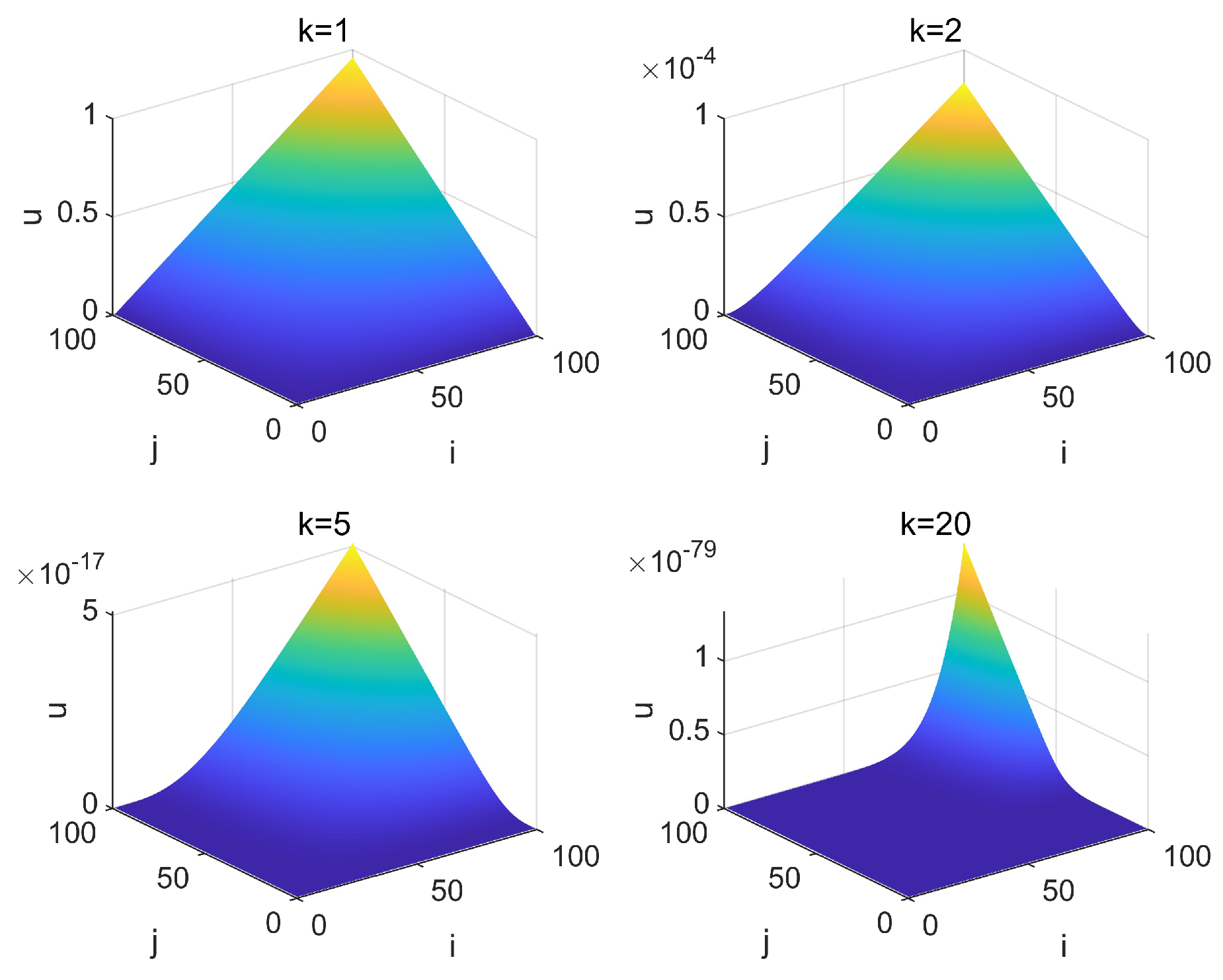
Based on the LMI criterion (10) with Q = 0 , S = 0 and R = I in the fastest learning mode, an optimal α * = 0.9976 is obtained with L = [ 5.0000 2.0169 ] and K = [ 1.9831 9.9999 ] . Figure 1 and Figure 2 illustrate the vertical state and the input trajectories at different iterations, respectively. The state and the input converge to zero as the iteration number k increases. At the 20th iteration, their amplitudes attain 10 79 . Compared with other conventional methods for the analysis and synthesis of 3-D systems in an iterative repetitive mode, the proposed method provides a more computationally effective tool for the controller design. For this system, conventional methods using the “lifting technique” will entail a test matrix for controller design whose matrix dimension would be multiples of 100 if we discrete the temperature distribution in space into state vectors with 100 points. This is a large computational burden. However, with the proposed method, the dimension of the test matrix for the control design is only 4, with the same number of space discretization steps. It can be easily solved within an extremely short time. The benefit is be clearer if more space discretization steps are required for accuracy in real applications. That is because the dimension would still be 4 with our method, while it would grow with the number of space discretization steps using other “lifting technique”-based schemes.
Additionally, the simulation is conducted with the proposed controller, whose parameters are randomly selected as L = [ 2.6924 1.0770 ] and K = [ 1.0770 5.4573 ] . These control parameters are feasible according to the condition (10). However, it can be seen from Figure 3 and Figure 4 that these provide a slower convergence rate. Indeed, the amplitudes of the vertical state and the input trajectories just attain the value of 10 8 at the 20th iteration. To further illustrate the comparison, an error index in the iteration direction is proposed as
E k = 1 T i T j i = 0 T i j = 0 T j y k T ( i , j ) y k ( i , j ) .
The error index is presented in Figure 5, which demonstrates that the proposed controller with the optimal parameters exhibits superior convergence performance.

4.2. ILC for Unstable Systems

Concerning the Roesser model, which is not asymptotically stable in the i and j dimensions, it is not possible to have A T P A P < 0 ; therefore, the condition (10) is not feasible. In this case, Theorems 2 and 3 provide sufficient conditions of stability in the iteration dimension, which can be used for the design of ILC. Consider the following numeric example:
x ¯ k ( i , j ) = 2 0 0 2 x k ( i , j ) + 1 0 0 1 u k ( i , j )
y k ( i , j ) = 1 0 0 1 x k ( i , j ) .
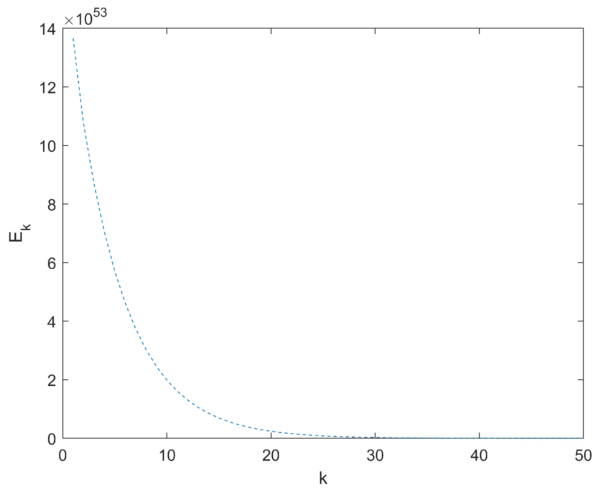
Using the LMI criterion (20) with Q = I , S = I and R = I , an optimal α * = 3.35 × 10 18 is derived with L = 0.2 0 0 0.2 and K = 0.1 0 0 0.1 . The error index E k for this controller is depicted in Figure 6. Despite the system being unstable (under zero input) in the i and j dimensions, iterative stability is achieved.

5. Conclusions

In this paper, we have presented a 3-D iterative dissipativity framework, under which the open-loop iterative learning control problem of the partial difference equation dynamics in repetitive processes is addressed. Firstly, the notion of iterative dissipativity is defined, and sufficient conditions in terms of LMI are derived. Subsequently, it is proved that the iterative dissipativity of a system implies its point-wise asymptotic stability in the iteration direction. We also argue that iterative dissipativity would preclude the system from degenerating from trial to trial. It is possible to obtain acceptable performances along the trial in any iteration if an appropriate initial iteration control input is selected. Thirdly, the open-loop ILC can be designed with optimal parameters that provide the fastest learning speed by utilizing LMI conditions. A thermal application in chemical engineering and a numeric example are presented to illustrate the proposed approach.

Funding

This research was partially funded by the National Natural Science Foundation of China (No: 61703444) and the Science and Technology Planning Project of Guangdong Province, China (No: 2021B1212040017).

Data Availability Statement

The original contributions presented in this study are included in this article; further inquiries can be directed to the corresponding author.

Conflicts of Interest

The authors declare no conflicts of interest.

References

  1. Lazebnik, T.; Alexi, A. High Resolution Spatio-Temporal Model for Room-Level Airborne Pandemic Spread. Mathematics 2023, 11, 426. [Google Scholar] [CrossRef]
  2. Kaczorek, T. Two-dimensional linear systems. In Proceedings of the Advances in Control; Frank, P.M., Ed.; Springer: London, UK, 1999; pp. 283–284. [Google Scholar]
  3. Ali, I.; Saleem, M.T. Spatiotemporal Dynamics of Reaction–Diffusion System and Its Application to Turing Pattern Formation in a Gray–Scott Model. Mathematics 2023, 11, 1459. [Google Scholar] [CrossRef]
  4. Xu, K.; Li, H.; Yang, H. Local-properties-embedding-based nonlinear spatiotemporal modeling for lithium-Ion battery thermal process. IEEE Trans. Ind. Electron. 2018, 65, 9767–9776. [Google Scholar] [CrossRef]
  5. Zhang, L.; Liu, S. Iterative learning control for flexible manipulator using fourier basis function. Int. J. Autom. Comput. 2015, 12, 639–647. [Google Scholar] [CrossRef]
  6. Roesser, R. A discrete state-space model for linear image processing. IEEE Trans. Autom. Control 1975, 20, 1–10. [Google Scholar] [CrossRef]
  7. Xiao, T.; Li, H. Eigenspectrum-based iterative learning control for a class of distributed parameter system. IEEE Trans. Autom. Control 2017, 62, 824–836. [Google Scholar] [CrossRef]
  8. Arimoto, S. Mathematical Theory of Learning with Applications to Robot Control. In Adaptive and Learning Systems: Theory and Applications; Narendra, K.S., Ed.; Springer: Boston, MA, USA, 1986; pp. 379–388. [Google Scholar]
  9. Wang, Y.; Gao, F.; Doyle, F.J. Survey on iterative learning control, repetitive control, and run-to-run control. J. Process Control 2009, 19, 1589–1600. [Google Scholar] [CrossRef]
  10. Xu, Q.Y.; He, W.Y.; Zheng, C.T.; Xu, P.; Wei, Y.S.; Wan, K. Adaptive Fuzzy Iterative Learning Control for Systems with Saturated Inputs and Unknown Control Directions. Mathematics 2022, 10, 3462. [Google Scholar] [CrossRef]
  11. Attia, S.B.; Alzahrani, S.; Alhuwaimel, S.; Salhi, S.; Ouerfelli, H.E. Polynomial Iterative Learning Control (ILC) Tracking Control Design for Uncertain Repetitive Continuous-Time Linear Systems Applied to an Active Suspension of a Car Seat. Mathematics 2024, 12, 2573. [Google Scholar] [CrossRef]
  12. Wei, Y.; Ouyang, Y.; Shang, W. Higher-order iterative learning control for nonlinear continuous systems with variable input trail lengths and input saturation. Discret. Contin. Dyn. Syst. 2024, 17, 2912–2930. [Google Scholar] [CrossRef]
  13. Cichy, B.; Gałkowski, K.; Rogers, E.; Kummert, A. An approach to iterative learning control for spatio-temporal dynamics using nD discrete linear systems models. Multidimens. Syst. Signal Process. 2011, 22, 83–96. [Google Scholar] [CrossRef]
  14. Cichy, B.; Gałkowski, K.; Rogers, E. Iterative learning control for spatio-temporal dynamics using Crank-Nicholson discretization. Multidimens. Syst. Signal Process. 2012, 23, 185–208. [Google Scholar] [CrossRef]
  15. Dai, X.; Tian, S.; Guo, Y. Iterative learning control for discrete parabolic distributed parameter systems. Int. J. Autom. Comput. 2015, 12, 316–322. [Google Scholar] [CrossRef]
  16. Xiao, T.; Li, X.D. PID-type Iterative Learning Control for 2-D Roesser Model. In Proceedings of the 2017 6th Data Driven Control and Learning Systems, Chongqing, China, 26–27 May 2017; pp. 400–404. [Google Scholar]
  17. Wan, K.; Li, X. Iterative learning control for two-dimensional linear discrete systems with Fornasini-Marchesini model. Int. J. Control Autom. Syst. 2017, 15, 1710–1719. [Google Scholar] [CrossRef]
  18. Willems, J.C. Dissipative dynamical systems part I: General theory. Arch. Ration. Mech. Anal. 1972, 45, 321–351. [Google Scholar] [CrossRef]
  19. Willems, J.C. Dissipative dynamical systems Part II: Linear systems with quadratic supply rates. Arch. Ration. Mech. Anal. 1972, 45, 352–393. [Google Scholar] [CrossRef]
  20. Hill, D.J.; Moylan, P.J. Stability results for nonlinear feedback systems. Automatica 1977, 13, 377–382. [Google Scholar] [CrossRef]
  21. Tan, Z.Q.; Soh, Y.C.; Xie, L.H. Dissipative control for linear discrete-time systems. Automatica 1999, 35, 1557–1564. [Google Scholar] [CrossRef]
  22. Ahn, C.K.; Shi, P.; Basin, M.V. Two-dimensional dissipative control and filtering for roesser model. IEEE Trans. Autom. Control 2015, 60, 1745–1759. [Google Scholar] [CrossRef]
  23. Pakshin, P.; Emelianova, J.; Emelianov, M.; Galkowski, K.; Rogers, E. Passivity based stabilization of repetitive processes and iterative learning control design. Syst. Control Lett. 2018, 122, 101–108. [Google Scholar] [CrossRef]
  24. Emelianova, J.; Pakshin, P.; Galkowski, K.; Rogers, E. Dissipative stabilization of nonlinear repetitive processes with an iterative learning control application. In Proceedings of the 2019 American Control Conference (ACC), Philadelphia, PA, USA, 10–12 July 2019; pp. 2861–2866. [Google Scholar]
  25. Ghanbari, V.; Duenas, V.H.; Antsaklis, P.J.; Dixon, W.E. Passivity-based iterative learning control for cycling induced by functional electrical stimulation with electric motor assistance. IEEE Trans. Control Syst. Technol. 2019, 27, 2287–2294. [Google Scholar] [CrossRef]
  26. Ahn, H.; Chen, Y.; Moore, K.L. Iterative Learning Control: Brief Survey and Categorization. IEEE Trans. Syst. Man Cybern. Part C Appl. Rev. 2007, 37, 1099–1121. [Google Scholar] [CrossRef]
  27. Cichy, B.; Augusta, P.; Gałkowski, K.; Rauh, A.; Aschemann, H.; Rogers, E.; Rehák, B. Modeling and Iterative Learning Control of a Circular Deformable Mirror. IFAC-PapersOnLine 2017, 50, 3117–3122. [Google Scholar] [CrossRef]
  28. Boyd, S.; El Ghaoui, L.; Feron, E.; Balakrishnan, V. Linear Matrix Inequalities in System and Control Theory; Studies in Applied and Numerical Mathematics; Society for Industrial and Applied Mathematics: Philadelphia, PA, USA, 1994; p. 194. [Google Scholar]
  29. Gahinet, P.; Nemirovskii, A.; Laub, A.J.; Chilali, M. The LMI control toolbox. In Proceedings of the 1994 33rd IEEE Conference on Decision and Control, Lake Buena Vista, FL, USA, 14–16 December 1994; pp. 2038–2041. [Google Scholar]
  30. Du, C.; Xie, L. H Control and Filtering of Two-Dimensional Systems; Lecture Notes in Control and Information Sciences; Springer: Berlin/Heidelberg, Germany, 2002; p. 152. [Google Scholar]
  31. El-Agizi, N.; Fahmy, M. Two-dimensional digital filters with no overflow oscillations. IEEE Trans. Acoust. Speech Signal Process. 1979, 27, 465–469. [Google Scholar] [CrossRef]
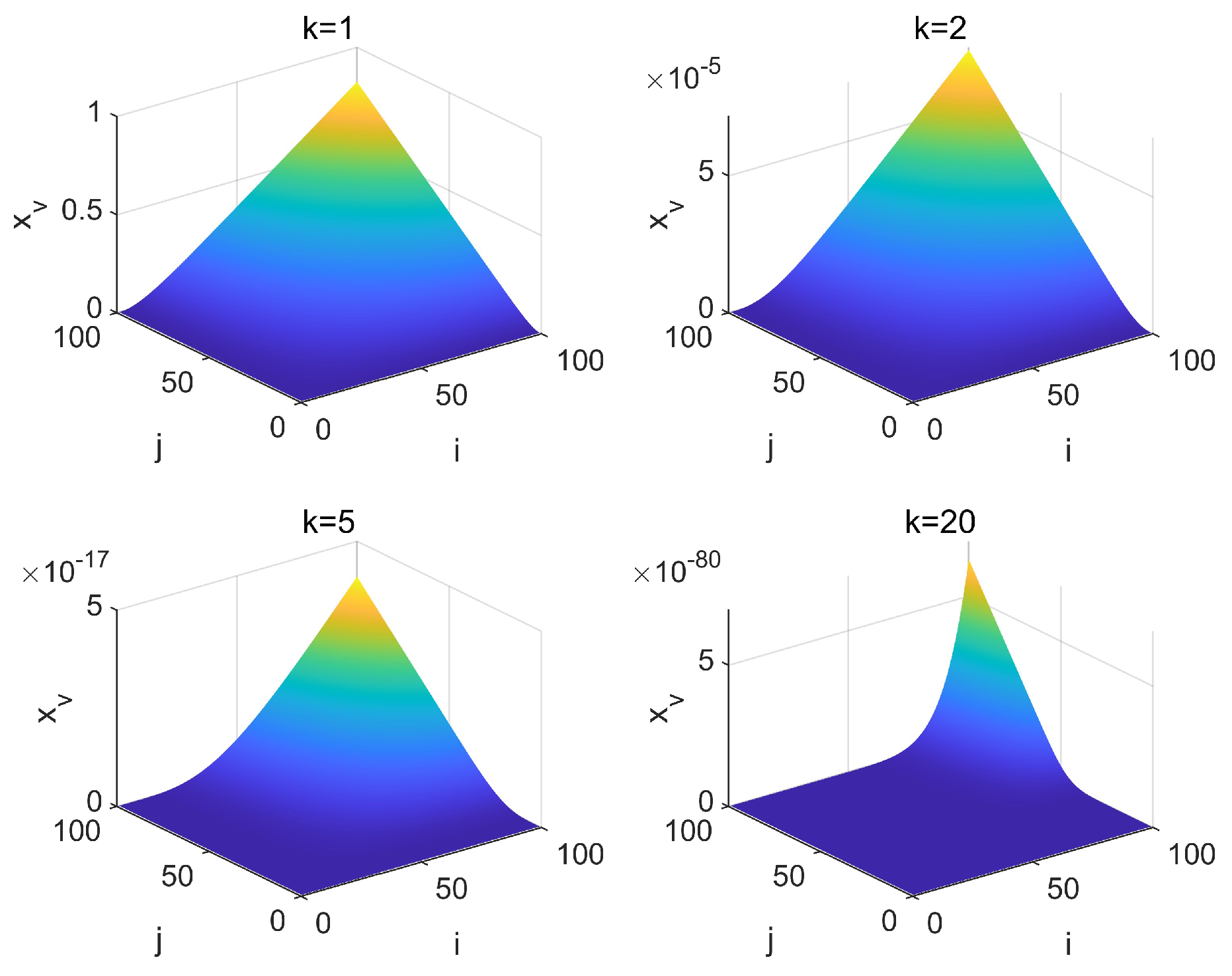
Figure 1. The vertical state trajectories x k v ( i , j ) at different iterations with optimal parameters.
Mathematics 12 03128 g001
Figure 2. The input trajectories u k ( i , j ) at different iterations with optimal parameters.
Mathematics 12 03128 g002
Figure 3. The vertical state trajectories x k v ( i , j ) at different iterations with random feasible parameters.
Mathematics 12 03128 g003
Figure 4. The input trajectories u k ( i , j ) at different iterations with random feasible parameters.
Mathematics 12 03128 g004
Figure 5. Error index E k in the iteration direction.
Mathematics 12 03128 g005
Figure 6. Error index E k in the iteration direction.
Mathematics 12 03128 g006
Disclaimer/Publisher’s Note: The statements, opinions and data contained in all publications are solely those of the individual author(s) and contributor(s) and not of MDPI and/or the editor(s). MDPI and/or the editor(s) disclaim responsibility for any injury to people or property resulting from any ideas, methods, instructions or products referred to in the content.