Applying the Simulated Annealing Algorithm to the Set Orienteering Problem with Mandatory Visits

Abstract

This study addresses the set orienteering problem with mandatory visits (SOPMV), a variant of the team orienteering problem (SOP). In SOPMV, certain critical sets must be visited. The study began by formulating the mathematical model for SOPMV. To tackle the challenge of obtaining a feasible route within time constraints using the original MILP approach, a two-stage mixed-integer linear programming (MILP) model is proposed. Subsequently, a simulated annealing (SA) algorithm and a dynamic programming method were employed to identify the optimal route. The proposed SA algorithm was used to solve the SOP and was compared to other algorithms, demonstrating its effectiveness. The SA was then applied to solve the SOPMV problem. The results indicate that the solutions obtained using SA are superior and more efficient compared to those derived from the original MILP and the two-stage MILP. Additionally, the results reveal that the solution quality deteriorates as the ratio of the set of mandatory visits increases or the maximum allowable travel time decreases. This study represents the first attempt to integrate mandatory visits into SOP, thereby establishing a new research direction in this area. The potential impact of this research is significant, as it introduces new possibilities for addressing complex combinatorial optimization problems.

1. Introduction

The Orienteering Problem (OP) is a complex NP-hard combinatorial optimization problem [1]. OP combines elements of the knapsack problem (KP) and the traveling salesman problem (TSP) [2]. The Team Orienteering Problem (TOP) is a variant of OP inspired by the popular outdoor sport of score orienteering. In this sport, participants use a compass and a map to visit marked points in an orderly manner, with the objective being to visit all points in the shortest time. Score orienteering requires participants to locate some or all points within a specified period, and the winner is the one with the highest score achieved in the least amount of time. Accordingly, OP can be described as finding a path that adheres to constraints, such as time and resources, while maximizing objectives, such as profit and satisfaction.

The goal of the OP is to maximize profit. To achieve this, the solution must include some, or at least one, of the points in the model graph. This necessitates selecting more “valuable” points and arranging them into paths that meet the specific constraints of the problem. Therefore, OP is a path problem focused on single-vehicle profitability. In this context, each customer point has an associated profit. The objective is to determine a single-vehicle route that maximizes the total profit from visited customers without exceeding the maximum time limit.

OP has diverse real-life applications, including courier delivery, ride-hailing services, urban tourism, bicycle sharing, communication network construction, industrial waste collection, salesman travel with time or distance constraints, school shuttle bus route planning, and civil aviation planning. Due to resource limitations, costs, and the high number of customer points, visiting all points is not always feasible. Therefore, the OP is extended to the Set Orienteering Problem (SOP).

Similar to SOP, the Clustered Orienteering Problem (COP) is another profitable path problem. COP requires visiting not just one point from each cluster, but all points within each cluster. The cluster’s profit is collected only when all the cluster customers are visited. This approach can reduce time and costs compared to OP’s application [3]. As a variation of OP, SOP retains OP’s goal but introduces additional considerations by grouping points into collections. To obtain the profit from a collection, at least one customer from each set must be visited. The problem entails finding a path within a subset of these collections such that: (i) the collected profit is maximized; (ii) the path length is within a specified range; and (iii) the travel time is within a given limit. For instance, when encountering multiple museums or theme parks of similar nature, one can select a few to visit, prioritizing those within the time constraints.

Previous literature has extensively discussed OP, including various articles and survey papers covering different OP variations [2,4]. SOP is a variant of OP that involves classifying points into similar groups. This problem can be likened to traveling to a new location and aiming to visit as many different types of tourist attractions as possible within a limited timeframe. Among attractions of the same type, the goal is to select the most convenient one to visit first and then proceed to the next most convenient different type of attraction. For example, starting from a hotel, one might visit the nearest attraction, followed by a temple. The nearest museum, and finally, maximize the visit to special attractions (i.e., maximize profit) within the allowable time while ensuring a timely return to the hotel. In some cases, certain sets must be visited in SOP, resulting in the Set Orienteering Problem with Mandatory Visits (SOPMV). Applications of SOPMV include planning road maintenance activities and designing tourist itineraries. To our knowledge, this problem has not been previously studied. Therefore, this study formulated a mixed integer linear programming (MILP) model for SOPMV and developed a simulated annealing algorithm to address it.

The main contributions of this study are as follows:

(1)

Development of a MILP model for SOPMV by modifying the existing SOP model;

(2)

Generation of benchmark problems for SOPMV based on the SOP problem set;

(3)

Application of a two-phase MILP approach to solving the SOPMV;

(4)

Utilization of a simulated annealing algorithm to solve the SOPMV;

(5)

Analysis of the effects of different ratios of mandatory visit sets.

The remainder of this paper is structured as follows. The next section reviews the literature on OP. Section 3 defines the problem and formulates its MILP model. Section 4 describes the two-phase MILP and the proposed SA algorithm. In Section 5, the effectiveness and efficiency of the proposed simulated annealing algorithm are empirically assessed using an existing benchmark problem set, and its performance is compared with that of state-of-the-art algorithms. Finally, Section 6 presents conclusions and recommendations for future research.

2. Literature Review

OP was first introduced by Tsiligirides [5], who described it as a variant of orienteering. The author defined orienteering as an outdoor sport where athletes compete to accumulate the most points. In this sport, athletes must navigate a field with designated start and finish points, where different access points are assigned varying point values. The objective is to visit as many points as possible within a specified time and maximize the total points accumulated. This cross-country sport challenges the athletes’ physical endurance and cognitive skills, such as planning ability and sense of direction. Golden [1] characterized OP as a complex NP-hard problem, noting that developing an exact solution algorithm is highly time-consuming and that heuristic algorithms are essential for solving practical problems. However, Gendreau and Laporte [6] argued that designing effective heuristic algorithms for OP is challenging. They argued that the vertex score and the time required to reach a vertex are often independent and contradictory and that simple design and refinement of heuristics may not effectively address the problem. Conversely, Gavalas and Konstantopoulos [7] maintained that OP is a specialized path optimization problem aimed at finding the optimal path under specific constraints to maximize benefits. Unlike other path problems, such as the traveling salesman problem or vehicle route planning, which focuses on minimizing total distance or cost, OP specifically targets profit maximization from selected paths. In OP, only some objective points need to be visited, while in traveling salesman problems and vehicle routing problems, all objective points must be included, and a general mathematical model has been derived.

The extensive research conducted by numerous scholars has significantly broadened the scope of OP studies, integrating various applications and algorithmic solutions [1,2,5,8,9,10,11]. Vansteenwegen and Souffriau [2] provided a comprehensive summary of relevant OP research, standardizing and unifying the mathematical descriptions of various OP variants. They reviewed several OP-related problems, including Team Orienteering Problem (TOP), Orienteering Problem with Time Windows (OPTW), and Team Orienteering Problem with Time Windows (TOPTW). Their analysis highlighted the use of heuristic algorithms to address these problems, emphasizing that many real-world issues can be effectively modeled as OP or its variants. In this way, problems can be solved very quickly and efficiently. They anticipate that the OP will increasingly influence tourism planning and other fields.

Researchers have organized and summarized studies on various OP variants, distinguishing between classical and nonclassical OPs [4]. Classical OPs, such as TOP, OPTW, and TOPTW, have been addressed using algorithms including Strengthened Particle Swarm Optimization (StPSO), Discrete Strengthened Particle Swarm Optimization (DSPSO), Approximation Algorithm (APA), and Approximation Algorithm (AA), such as Multilevel Variable Neighborhood Search (MLVNS), Greedy Randomized Adaptive Search Procedure, and Path Relinking Algorithms. Search Procedure and Path Relinking (GRASPPR), Memetic-Greedy Randomized Adaptive Search Procedure (MGRASP), Robust Branch-Cut-Price Algorithm (Robust Branch-Cut-Price Algorithm (RBCP), Genetic Algorithm (GA), and Memetic Algorithm (MA), which combines some local search techniques, Discrete Particle Swarm Optimization (DPSO), Branch-Cut-Price Algorithm for subset-inequalities, and Pareto Mimic Algorithm (PMA). In contrast, nonclassical OPs include variants such as the (1) Stochastic Orienteering Problem, (2) Generalized Orienteering Problem, (3) Arc Orienteering Problem, (4) Capacitated Team Orienteering Problem, (5) Orienteering Problem with Variable Profits, (6) Clustered Orienteering Problem, (7) Correlated Orienteering Problem, (8) Cooperative Orienteering Problem, (9) Multiagent Orienteering Problem, (10) Multiperiod OP with Multiple Time Windows, and (11) Multiconstraint TOP with Multiple Time Windows.

Gunawan and Lau [4] summarized these nonclassical OPs and their associated algorithms. They highlighted that solutions for these variants can be approached using methods such as the Branch-Cut-Price Algorithm, Branch-Cut Algorithm, and Tabu Search, Hybrid Greedy Randomized Adaptive Search Procedure, Iterative Operational Search Procedure, Algorithm, Branch-and-Cut Algorithm and Tabu Search, Hybrid Greedy Randomized Adaptive Search Procedure and Iterated Local Search, and Adaptive Large Neighborhood Search. Gunawan and Lau [4] concluded that further research should focus on cross-country search problem variants involving time-dependent travel times, multiple constraints, and multiple objectives. Developing effective solution algorithms for these challenging variants, combining exact algorithms and heuristic approaches, will be valuable for addressing similar problems in the future.

In a broader sense, different types of OPs vary in how profits are earned. In the classic OP, the profit associated with each point is specific to that point. However, in SOP, the profit can be obtained by reaching any point within a set or by visiting the set as a whole. Thus, SOP aims to maximize profit by covering as many sets as possible within the allowable time. Archetti and Carrabs [12] argued that SOPs are well-suited for scenarios where products are distributed in bulk, customers belong to different supply chains, and the carrier engages with the supply chain. In SOP, the carrier serves only one customer in each chain, implicitly serving the required quantity. This differs from the COP, where the carriers must serve all retailers within each chain as the contract specifies. Consequently, the SOP allows carriers to offer more competitive prices, as internal distribution among retailers in the chain is managed internally. Thus, SOP provides an alternative distribution strategy compared to COP, benefiting both the operators and the supply chain. Archetti and Carrabs [12] developed an exact algorithm for SOP, known as the MAtheuristic for the SOP, MASOP, which integrates the mathematical formulations of Tabu Search (TS) and Mixed-Integer Programming (MIP) with mathematical algorithms. Pěnička and Faigl [13] highlighted that SOP can be more profitable than OP by serving the entire set by visiting just one point within it. Therefore, they [13] applied a variable neighborhood search algorithm, VNS-SOP to SOP, demonstrating improved performance. Carrabs [14] proposed a genetic algorithm for solving SOPs using three local search processes to enhance biased random keying for solving chromosome fitness. This algorithm achieved results significantly faster than the algorithms proposed by Archetti, Carrabs [12], and Pěnička, Faigl [13] and obtained values very close to those of the other algorithms. Dontas and Sideris [15] introduced a mathematical algorithm based on local search to solve SOPs, which, through extensive experiments, yielded better results than the leading open-source SOP algorithms of its time. Yu, Salsabila [16] proposed the Set Team Orienteering Problem with Time Windows (STOPTW), a new variant of the well-known Team Orienteering Problem with Time Windows and Set Orienteering Problem. In the STOPTW, customers are grouped into sets. Each set is associated with a profit when any customer in the sets is visited within the customer’s time window. Dutta and Barma [17] formulated a multiobjective set-orienteering problem that provides a more realistic representation of real-world scenarios compared to existing models. In this problem, they incorporate two key features: (i) a predefined profit associated with each set of customers and (ii) a preset maximum service time associated with each customer within all the sets.

Palomo-Martínez and Salazar-Aguilar [18] introduced the orienteering problem with mandatory visits (OP-MV) as a variant of OP. They extend the classical problem by considering mandatory visit points and incorporating constraints related to the exclusion between nodes. Specifically, the OP-MV requires finding a route that visits all mandatory nodes and some optional nodes while ensuring that the total duration does not exceed a pre-specified time limit. The goal is to maximize the total number of points collected. For each optional node, an associated non-negative score is awarded only if that node is visited. Palomo-Martínez and Salazar-Aguilar solved OP-MV using a hybrid variable neighborhood search approach. Using a memetic algorithm, Lu and Benlic [19] solved the OP with mandatory visits and exclusionary constraints. Lin and Yu [20] addressed the TOPTW with mandatory visits by employing multistart simulated annealing (MSA).

3. The Problem Definition

The SOPMV can be defined on a directed network $G=\left(N,A\right)$, where $N=\left\{\mathrm{1,2},\dots ,n\right\}$ represents the set of nodes, and $A=\left\{\left(i,j\right):i\ne j\in N\right\}$ represents the set of arcs connecting nodes. Nodes in N are grouped into set S_k with k = 1, …, ns such that ${\cup }_{k=1}^{ns}{S}_k=S$ and $S_h\cap S_k=\varnothing$, $\forall S_h,S_k\in S$, where $S=\left\{S_1,S_2,S_3,\dots ,S_{ns}\right\}$ is the set of sets. A profit $P_k$ is associated with each set and is collected if and only if at least a node $i\in S_k$ is visited in the tour. The profit of each set can be collected at most once. As in the MILP of SOP [12], the objective is to find the tour that maximizes the collected profit. The traveling time t_ij required to travel from node i to j is known for each pair of nodes i and j. The total travel time of a tour should not exceed the given time budget T_max.

The following defines the parameters and decision variables:

• Parameter:

n	Number of nodes
ns	Number of sets
m	Number of sets with mandatory visits
M	The set of sets with mandatory visits
S	Set of all sets
Sk	Set k
i, j	Node indices
k	Set index
pk	Profit of set k
Tmax	Time limitation of the tour

• Decision Variable:

$x_{ij}=1$	If a visit to node i is followed by a visit to node j; 0 otherwise
$y_i=1$	If node i is visited; 0 otherwise
$z_k=1$	If set k is visited; 0 otherwise
$u_{ij}$	Auxiliary variables used to avoid subtours

The MILP of SOPMV can be formulated by extending the MILP of SOP [12] as follows:

• Objective Function:

$$P=max\sum _{k=1}^{ns}{p}_k{z}_k$$

(1)

Constraint:

$${\displaystyle \sum _{j=1}^n}{x}_{ij}=y_i i=1,2,\dots ,n$$

(2)

$${\displaystyle \sum _{i=1}^n}{x}_{ji}=y_i i=1,2,\dots ,n$$

(3)

$$z_k=1 k\in M$$

(4)

$$z_k\le {\displaystyle \sum _{i\in S_k}}{y}_i S_k\in S$$

(5)

$${\displaystyle \sum _{i=1}^n}{\displaystyle \sum _{j=1;i\ne j}^n}{t}_{ij}{x}_{ij}\le T_{max}$$

(6)

$${\displaystyle \sum _{j\in V}}{u}_{ji}-{\displaystyle \sum _{j\in V}}{u}_{ij}=y_i i\in V\backslash \left\{1\right\}$$

(7)

$$u_{ij}\le \left(\mathrm{n}-1\right)x_{ij} \left(i,j\right)\in A$$

(8)

The objective function (1) maximizes the total score collected from all paths. Constraint (2) ensures that if the vehicle travels from node i to node j, then node i must be visited. Constraint (3) ensures that if the vehicle travels from node j to node i, then node i must be visited. Constraint (4) mandates that all sets with mandatory visits must be included in the tour. Constraint (5) specifies that a set is considered visited if at least one vertex within that set is visited. Constraint (6) ensures that the duration of each tour does not exceed the specified time limit. Constraints (7) and (8) prevent the formation of subtours. The performance of this formulation of subtour elimination constraints for the Traveling Salesman Problem (TSP) had been evaluated by Öncan, Altınel [21].

4. The Proposed Algorithms

This study introduces a two-stage MILP and develops a simulated annealing heuristic to address the SOPMV. The following subsections provide a detailed discussion of the two-stage MILP for solving the SOPMV in detail and the proposed SA algorithm. Initially, the presentation of the solution, dynamic programming aspects, initial solutions, and neighborhood solutions for the proposed SA algorithm are described. Subsequently, the related parameters and implementation procedure of the proposed SA algorithm are outlined.

4.1. Two-Phase MILP for Solving SOPMV

The MILP formulation for SOVMV can effectively find the optimal solution for small-scale problems. However, as the problem size increases, finding the optimal solution within a finite time becomes challenging. In some cases, it is even difficult to generate a feasible solution.

This study proposes a two-stage MILP, denotes as MILP*, to solve the SOPMV and address this issue. In the first stage, the MILP only considers sets with mandatory visits. Due to the reduced problem size compared to the original formulation, obtaining an optimal or feasible solution is more manageable. In the second stage, the solution from the first stage is used as an initial solution for the MILP of the full SOPMV. Consequently, the second stage at least guarantees a feasible solution, and it has the potential to yield a better or optimal solution based on the initial solution provided by the first stage.

4.2. Solution Representation of SA

A solution $\pi$ is represented as a string of n numbers that denotes the permutation of sets. The sequence of these numbers indicates the preferred order in which the sets are to be served. The first number in the solution corresponds to the first set to be served, and subsequent sets are added to the tour in the order they appear from left to right, ensuring that the time limit is not exceeded. The specific node to be visited within each served set is determined using dynamic programming, as discussed later.

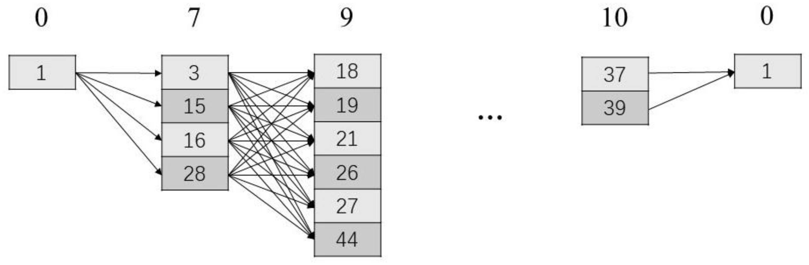
Table 1 presents a small example of a problem with SOPMV with 11 sets (44 nodes). In this example, Set 0 includes Node 1, which is referred to as the deposit. A sample solution for this problem is Π$=\left(7,9,4,3,10,5,2,11,8,6,1\right).$

Table 1. A small SOPMV example problem.

Set	Profit	Nodes in the Set	Mandatory Visit
0	0	1	-
1	3	11, 12, 46	No
2	3	2, 5, 36	No
3	5	6, 7, 8, 17, 35	No
4	13	4, 13, 14, 20, 22, 29, 31, 33, 34, 38, 40, 42, 43	No
5	1	30	No
6	1	41	No
7	4	3, 15, 16, 28	Yes
8	2	9, 45	No
9	6	18, 19, 21, 26, 27, 44	Yes
10	2	37, 39	Yes
11	4	10, 23, 24, 25	No

Given the sequence of set visits, determining which node within each set should be served to achieve the shortest distance path is known as the stagecoach problem, which can be addressed using dynamic programming [13,22]. For the given sequence Π $=\left(7,9,4,3,10,5,2,11,8,6,1\right),$ dynamic programming first solves the set visited sequence: 0-7-0. It then solves 0-7-9-0, 0-7-9-4-0, 0-7-9-4-3-0, and 0-7-9-4-3-10-0. While dynamic programming can calculate the traveling distance and identify the visiting node for each served set, it cannot provide a feasible solution for the sequence 0-7-9-4-3-10-5-0; no set can be served following set 10. Figure 1 illustrates the dynamic programming process for the SOPMV solution example (served set sequence: 0-7-9-4-3-10-0). 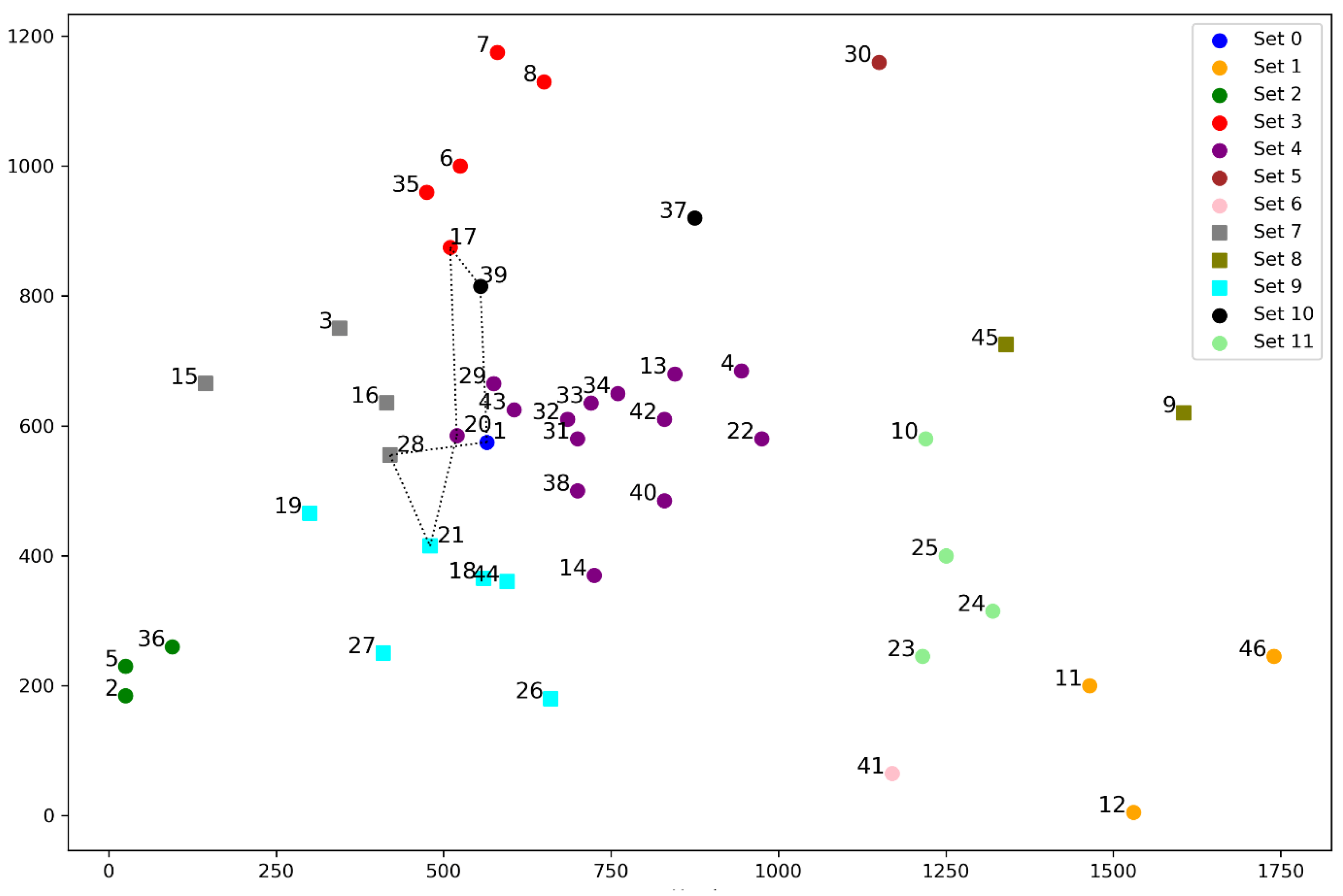Table 2 lists the visiting nodes for each served set. A visual representation of this solution example is provided in Figure 2.

Figure 1. The visual illustration of the dynamic programming.

Table 2. The nodes visited by the served sets (0-7-9-4-3-10-0).

Set No	0	7	9	4	3	10	0
Node No	1	28	21	20	17	39	1

Figure 2. The visual solution of the sample example.

4.3. Initial Solution of SA

To obtain a feasible initial solution, all sets with mandatory visits need to be served as much as possible. The initial solution is generated by the following steps.

(1)

First, add all sets with mandatory visits to the part of the initial solution (${\mathsf{\Pi }}_{part})$ in order of set number;

(2)

Then, add all other sets (sets without nonmandatory visits) to the ${\mathsf{\Pi }}_{part}$ in the order of set number, then a full initial solution ${\mathsf{\Pi }}_{init}$ can be obtained;

(3)

Exchange two sets with mandatory visits in ${\mathsf{\Pi }}_{init}$ one by one. If exchanging two sets with mandatory visits will improve the objective function, perform this exchange to obtain new ${\mathsf{\Pi }}_{init}$ and perform another exchange. This step is performed until the ${\mathsf{\Pi }}_{init}$ can be improved.

(4)

Finally, the ${\mathsf{\Pi }}_{init}$ is output as the initial solution. If any mandatory visit set remains unserved, a penalty of −999 is added to the objective function value of ${\mathsf{\Pi }}_{init}$ for each unserved mandatory set.

4.4. Neighborhood Solutions of SA

To generate a neighborhood solution from the current solution ${\mathsf{\Pi }}_{cur}$, three types of random moves are employed: insertion, swapping, and reversal. Each iteration produces a new solution ${\mathsf{\Pi }}_{new}$. The insertion move involves randomly selecting an element from ${\mathsf{\Pi }}_{cur}$ and placing it immediately before another randomly chosen element. The swap moves entail randomly selecting two sets and exchanging their positions. The inversion move involves selecting a random subsequence of ${\mathsf{\Pi }}_{cur}$ is selected and reversing its order. Each type of move—insertion, swap, and inversion—is chosen with an equal probability of 1/3. Because the codes for the set with mandatory visits are initially placed at the beginning of the solution representation, the neighborhood solution initially focuses only on changing the order of sets with mandatory visits in the current solution to generate a temporary solution. Once a feasible solution is found, the order of all sets can be adjusted.

4.5. Parameters Used and Procedure of the Proposed SA

The proposed simulated annealing heuristic involves four parameters: $T_0$, the initial temperature; $Ite{r}_{temp}$, the number of iterations at a given temperature; $\mathsf{\alpha },$ the coefficient that controls the cooling schedule; and ${Max}_{time},$ the maximal computational time. The algorithm is described in detail as follows.

At the beginning of the proposed SA heuristic, the current temperature (T) is set to the initial temperature $T_0$. After generating a feasible solution ${\mathsf{\Pi }}_{init}$, both the incumbent solution (${\mathsf{\Pi }}_{cur}$) and the best solution (${\mathsf{\Pi }}_{best}$) are initialized to ${\mathsf{\Pi }}_{init}$. The objective function value of ${\mathsf{\Pi }}_{cur}$ is calculated as $OF\left({\mathsf{\Pi }}_{cur}\right)$. If any set with mandatory visits is not served, a penalty of −999 is added to the objective function value. The following loop is executed until the computational time exceeds ${Max}_{time}.$ At each temperature iteration, a new neighborhood solution ${\mathsf{\Pi }}_{new}$ is generated according to the neighborhood search mechanism described in Section 4.4. Let $\mathsf{\Delta }$ represent the difference in objective function values between the new neighborhood solution ${\mathsf{\Pi }}_{new}$ and the incumbent solution ${\mathsf{\Pi }}_{cur}$, i.e., $\mathsf{\Delta }=OF\left({\mathsf{\Pi }}_{cur}\right)-OF\left({\mathsf{\Pi }}_{new}\right)$ If $∆>0$, then the new neighborhood solution ${\mathsf{\Pi }}_{new}$ will replace the incumbent solution ${\mathsf{\Pi }}_{cur}$; otherwise, the new neighborhood solution ${\mathsf{\Pi }}_{new}$ will replace the incumbent solution ${\mathsf{\Pi }}_{cur}$ if a random number $rand$ (between 0 and 1) is less than $e^{\left({\displaystyle \frac{∆}{\mathrm{T}}}\right)}$. If the new solution ${\mathsf{\Pi }}_{new}$ in the neighborhood meets these conditions, ${\mathsf{\Pi }}_{new}$ is replaced as the incumbent solution ${\mathsf{\Pi }}_{cur}$. The current temperature drops to $\mathsf{\alpha }T$, 0 < $\mathsf{\alpha }$ < 1, after $Ite{r}_{temp}$ iterations at the current temperature T. The best solution (${\mathsf{\Pi }}_{best}$) and its objective function value ($OF{V}_{best}$) are updated whenever a better feasible solution is found. The final best solution is derived from ${\mathsf{\Pi }}_{best}$ when the algorithm terminates. Algorithm 1 presents the pseudocode of the proposed SA heuristic for SOPMV, denoted as SA-SOPMV.

Algorithm 1: The pseudocode of SA-SOPMV
	Input: $T_0$, $\mathsf{\alpha }$, $I_{iter}$, ${Max}_{time}$
1	$T\leftarrow T_0$
2	${\Pi }_{init}\leftarrow$ Generate an initial solution
3	${\mathsf{\Pi }}_{cur}\leftarrow {\Pi }_{init}$
4	${\Pi }_{best}\leftarrow {\Pi }_{init}$
5	While ($Runnin{g}_{Time}<{Max}_{time})$
6	For $i=1$ to $I_{iter}$ do
7	$\hspace{1em}\hspace{1em}\hspace{1em}\hspace{1em}\hspace{1em}{\mathsf{\Pi }}_{new}\leftarrow$ Neighborhood solution of ${\mathsf{\Pi }}_{cur}$;
8	$\hspace{1em}\hspace{1em}\hspace{1em}\hspace{1em}\hspace{1em}\hspace{1em}\hspace{1em}\mathsf{\Delta }=OF\left({\mathsf{\Pi }}_{cur}\right)-OF\left({\mathsf{\Pi }}_{new}\right)$;
9	If $(\mathsf{\Delta }\ge 0)$ then
10	$\hspace{1em}\hspace{1em}\hspace{1em}\hspace{1em}\hspace{1em}\hspace{1em}\hspace{1em}\hspace{1em}\hspace{1em}{\mathsf{\Pi }}_{cur}\leftarrow {\mathsf{\Pi }}_{new}$;
11	If ${OF(\mathsf{\Pi }}_{new})\ge {OF(\mathsf{\Pi }}_{best})\mathrm{T}$ hen
12	$\hspace{1em}\hspace{1em}\hspace{1em}\hspace{1em}\hspace{1em}\hspace{1em}\hspace{1em}\hspace{1em}\hspace{1em}\hspace{1em}\hspace{1em}{\mathsf{\Pi }}_{best}\leftarrow {\mathsf{\Pi }}_{new}$;
13	Else
14	Random rand $\in \left[\mathrm{0,1}\right]$;
15	If ${exp}^{(\mathsf{\Delta }/T)}>rand$ then
16	$\hspace{1em}\hspace{1em}\hspace{1em}\hspace{1em}\hspace{1em}\hspace{1em}\hspace{1em}\hspace{1em}\hspace{1em}\hspace{1em}\hspace{1em}{\mathsf{\Pi }}_{cur}\leftarrow {\mathsf{\Pi }}_{new}$;
17	$\hspace{1em}\hspace{1em}\hspace{1em}\hspace{1em}\hspace{1em}i\leftarrow i+1$
18	$\hspace{1em}\hspace{1em}\hspace{1em}\hspace{1em}T\leftarrow T\ast \mathsf{\alpha }$
19	Return ${\mathsf{\Pi }}_{best}$

5. Computational Result

The proposed SA algorithm was implemented in C++. The experiments were conducted on a computer equipped with an Intel Core 3.40 GHz CPU. The mathematical programming model for SOPMV was solved using a Gurobi solver (Version 10.3) on the same machine.

5.1. Problem Set Used

The SOPMV problem set used in this study was derived from the SOP problem sets presented by Archetti and Carrabs [12] and Pěnička and Faigl [13]. Two problem sets were utilized. The first set comprised 20 problem instances (referred to as the small GTSP dataset instances in the original studies), while the second set contained 47 × 2 problem instances (referred to as the large GTSP dataset instances of SOP with ω = 1, where ω is used to compute the tour’s time limit). In these problems, the number of nodes ranged from 52 to 1084. The number of sets in each problem equals 20% of the total number of customers. The distance between nodes was calculated using the Euclidean distance between nodes’ coordinates, with the result rounded up to the nearest integer. A parameter Pg determines the profit generation rule. Specifically, Pg = g1 if the profit of each set Sg is equal to |Sg|. If Pg = g2, the profit of node j is calculated as (1 + (7141j + 73) mod 100) to generate pseudo-random profits. The profit of a set is then obtained by summing the profits of all its constituent nodes. For detailed descriptions of the SOP problem sets, refer to Archetti and Carrabs [12] and Pěnička and Faigl [13].

The SOPMV problem set was generated as follows: First, any unused metadata from the original problem file was discarded. A binary value was appended to each set in the file, where 1 indicates a mandatory visit and 0 indicates otherwise. After specifying the number of sets with mandatory visits, a unique set of the required number was randomly selected as mandatory.

Given the challenges in generating problems with feasible solutions when the ratios of sets with mandatory visits are too high for the first problem set, three ratios were used: 10%, 20%, and 30% (denoted as 10%MV, 20%MV, and 30%MV) with W values kept unchanged from the original SOP problems. Consequently, there are 20×3×1 = 60 problems in the first problem set of SOPMV. For the second problem set, three ratios % of MV values (10%, 20%, and 30%) and three ω values (0.4, 0.6, and 0.8) were utilized, resulting in 94×3×3 = 846 problems in SOPMV.

5.2. Parameter Calibration

The proposed SA algorithm is governed by four key parameters: ST, $I_{iter}$, CR, and ${Max}_{time}$. Here, ST denotes the starting temperature; $I_{iter}$ denotes the number of iterations at a specific temperature; CR is the cooling rate, and ${Max}_{time}$ is the maximum allowable computational time measured in seconds. Given the significant impact of these parameters on the quality of computational results, careful selection of their values is essential. Table 3 outlines the four levels of each parameter, and the 16 parameter combinations used in the SA algorithm. Taguchi’s L16 orthogonal experimental design was employed to optimize these parameters, and each of the four randomly selected problem instances was executed ten times.

Table 3. Orthogonal array and the obtained ARPDs.

No	ST	CR	${\mathit{I}}_{\mathit{i}\mathit{t}\mathit{e}\mathit{r}}$	${\mathit{M}\mathit{a}\mathit{x}}_{\mathit{t}\mathit{i}\mathit{m}\mathit{e}}$	APRD
1	7	0.99	70,000	0.5*NSet	0.5299%
2	7	0.97	80,000	1.0*NSet	0.2734%
3	7	0.95	90,000	1.5*NSet	0.2409%
4	7	0.93	100,000	2.0*NSet	0.1575%
5	10	0.99	80,000	1.5*NSet	0.1734%
6	10	0.97	70,000	2.0*NSet	0.2197%
7	10	0.95	100,000	0.5*NSet	0.4225%
8	10	0.93	90,000	1.0*NSet	0.3619%
9	13	0.97	90,000	2.0*NSet	0.2291%
10	13	0.95	100,000	1.5*NSet	0.2490%
11	13	0.93	70,000	1.0*NSet	0.2386%
12	13	0.99	80,000	0.5*NSet	0.3127%
13	16	0.99	100,000	1.0*NSet	0.2426%
14	16	0.97	90,000	0.5*NSet	0.3723%
15	16	0.95	80,000	2.0*NSet	0.2160%
16	16	0.93	70,000	1.5*NSet	0.1030%

*: NSet denotes the number of sets.

The average relative percentage deviation (ARPD) from the best objective function value (total collected profit) for each instance is presented in Table 3 and Table 4. The relative percentage deviation (RPD) was calculated using the following formula:

$$ARPD=\left(\sum _{r=1}^4{\displaystyle \frac{{P_r}_{best}-P_r}{{P_r}_{best}}}\times 100\%\right)÷4$$

(9)

where $P_r$ denotes the average objective function value (total collected profit) of a specific problem instance $i$ ($i=1,...,4$) obtained from 10 runs using the proposed SA algorithm with a given parameter combination, and ${P_r}_{best}$ is the best total collected profit obtained for that problem instance from $4\times 16=160$ runs using all parameter combinations of the proposed SA algorithm.

Table 4. ARPDs obtained by different levels of each parameter.

Setting	ST	CR	TI	${\mathit{M}\mathit{a}\mathit{x}}_{\mathit{t}\mathit{i}\mathit{m}\mathit{e}}$
1	0.3004%	0.2153%	0.2728%	0.4093%
2	0.2944%	0.2821%	0.2439%	0.2791%
3	0.2573%	0.2736%	0.3010%	0.1916%
4	0.2335%	0.3146%	0.2679%	0.2056%
Range	0.0670%	0.0994%	0.0572%	0.2178%
Rank	3	2	4	1

The ARPDs obtained using different parameter settings are shown in Table 4. These results indicate that ${Max}_{time}$ is the most influential parameter. Longer execution times generally lead to better objective function values. Assessing the effects of ST, CR, and $I_{iter}$ separately proved challenging. Typically, a high ST requires more computational time to achieve better solutions, while a low ST may lead to premature convergence due to the low acceptance probability. A high CR results in a slower temperature reduction, while a low CR leads to a rapid temperature decrease. Additionally, the number of iterations at the same temperature affects the computational time at that specific temperature. The final parameter values are set to 16, 0.93, 80,000, and 1.5*Nset (seconds) to balance quality and computational time. These values represent the starting temperature, cooling rate, number of iterations at the same temperature, and the maximum allowable computational time in seconds.

5.3. Solving the SOP

Since MASOP [12] and VNS-SOP [13] have addressed the SOP problem instances utilized in this study, the performance of the SA-SOPMV algorithm can be directly compared with MASOP and VNS-SOP. In scenarios where the SOPMV problem instance lacks any sets with mandatory visits, it effectively reduces to an SOP problem, which the SA-SOPMV algorithm can still solve efficiently.

5.3.1. Solving the First SOP Problem Set

The results of solving the 20 instances in the first SOP problem set are summarized in Table 5. All the MASOP, VNS-SOP, SA-SOPMV, and MILP can obtain the best solutions. Although the proposed SA algorithm requires more computing time than VSN-SOP, it successfully identifies all optimal solutions. The maximum allowable computational time for MILP is set to 14,400 s.

Table 5. The result of solving the first SOP problem set.

Instance	Pg	W	Tmax	MILP		MASOP		VNS-SOP		SA-SOPMV
				P	T	P	T	P	T	P	AVE P	T
11berlin52	g1	0.4	1616	37	47.07	37	1.75	37	0.11	37	37	2.2
11berlin52	g2	0.4	1616	1829	65.96	1829	1.70	1829	0.11	1829	1829	2.2
11berlin52	g1	0.6	2424	43	777.88	43	2.40	43	0.16	43	43	2.2
11berlin52	g2	0.6	2424	2190	1532.91	2190	2.64	2190	0.15	2190	2190	2.2
11berlin52	g1	0.8	3232	47	2648.04	47	7.17	47	0.19	47	47	2.2
11berlin52	g2	0.8	3232	2384	3833.50	2384	6.61	2384	0.19	2384	2384	2.2
11eil51	g1	0.4	69	24	39.72	24	1.85	24	0.09	24	24	2.2
11eil51	g2	0.4	69	1279	40.13	1279	1.97	1279	0.09	1279	1279	2.2
11eil51	g1	0.6	104	39	34.64	39	5.13	39	0.14	39	39	2.2
11eil51	g2	0.6	104	1911	204.65	1911	4.74	1911	0.14	1911	1911	2.2
11eil51	g1	0.8	139	43	1586.67	43	2.3	43	0.18	43	43	2.2
11eil51	g2	0.8	139	2114	1520.67	2114	1.93	2114	0.20	2114	2114	2.2
14st70	g1	0.4	126	33	9666.29	33	4.43	33	0.14	33	33	2.8
14st70	g2	0.4	126	1672	4396.77	1672	4.35	1672	0.15	1672	1672	2.8
14st70	g1	0.8	252	65	14,400.00	65	8.8	65	0.31	65	65	2.8
14st70	g2	0.8	252	3355	14,400.00	3355	7.89	3355	0.33	3355	3355	2.8
16eil76	g1	0.4	83	40	4987.09	40	3.88	40	0.19	40	40	3.2
16eil76	g2	0.4	83	2223	4939.08	2223	4.73	2223	0.20	2223	2223	3.2
16eil76	g1	0.6	125	59	14,400.00	59	2.40	59	0.31	59	59	3.2
16eil76	g2	0.6	125	3119	14,400.00	3119	6.28	3119	0.32	3119	3119	3.2

5.3.2. Solving the Second SOP Problem Set

Table 6 presents the results for the 94 instances in the second SOP problem set. Despite requiring more computational time than VSN-SOP, the SA-SOP algorithm achieves solutions that are either equal to or very close to those obtained by VSN-SOP. The range of ARPD for each individual instance is from −1.946% to 2.568%.

Table 6. The result of solving the second SOP problem set.

Instance	g1								g2
	MSAOP		VNS-SOP			SA-SOP			MSAOP		VNS-SOP			SA-SOP
	P	T	P	Pavg	T	P	Pavg	T	P	T	P	Pavg	T	P	Pavg	T
16pr76	74	8.6	74	74.0	0.6	74	74.0	24.0	3765	10.6	3765	3765.0	0.6	3765	3765.0	24.0
20kroA100	96	10.5	96	96.0	0.8	96	96.0	30.0	4868	11.5	4868	4868.0	0.8	4868	4868.0	30.0
20kroB100	98	13.4	98	98.0	0.8	98	98.0	30.0	4916	10.7	4916	4916.0	0.9	4916	4916.0	30.0
20kroC100	97	10.8	97	96.1	0.9	97	97.0	30.0	4882	11.2	4882	4869.2	1.1	4882	4882.0	30.0
20kroD100	96	10.3	96	96.0	1.0	96	96.0	30.0	4838	8.9	4838	4838.0	1.1	4838	4792.4	30.0
20kroE100	96	9.1	96	96.0	0.9	96	96.0	30.0	4887	9.9	4887	4887.0	1.1	4887	4876.2	30.0
20rat99	93	7.6	93	92.9	1.2	93	93.0	30.0	4721	8.1	4721	4721.0	1.0	4721	4721.0	30.0
20rd100	97	10.4	97	97.0	1.3	97	97.0	30.0	4929	9.6	4929	4929.0	1.3	4929	4924.4	30.0
21eil101	97	8.8	98	97.8	1.2	98	98.0	31.5	4953	20.1	4993	4957.0	1.1	4948	4940.0	31.5
21lin105	102	8.1	102	102.0	1.1	102	102.0	31.5	5157	8.4	5157	5157.0	1.1	5157	5140.8	31.5
22pr107	101	8.6	101	101.0	0.6	101	101.0	33.0	5109	8.3	5109	5105.4	0.7	5101	5089.6	33.0
25pr124	121	11.3	121	121.0	1.3	121	121.0	37.5	6173	11.9	6173	6170.2	1.5	6173	6154.0	37.5
26bier127	125	16.0	125	125.0	1.8	125	125.0	39.0	6314	16.2	6314	6314.0	1.8	6314	6314.0	39.0
26ch130	127	10.2	127	126.7	1.9	127	127.0	39.0	6412	9.7	6412	6382.3	2.2	6412	6383.8	39.0
28pr136	134	10.2	134	134.0	2.1	134	134.0	42.0	6841	12.2	6841	6831.4	1.8	6841	6836.2	42.0
29pr144	141	17.4	141	141.0	1.7	141	141.0	43.5	7195	22	7195	7157.3	1.6	7137	7134.6	43.5
30ch150	144	9.6	147	146.7	2.1	147	147.0	45.0	7315	12.3	7394	7378.2	1.9	7394	7362.2	45.0
30kroA150	145	11.3	145	144.7	2.2	145	145.0	45.0	7361	13.8	7361	7356.6	2.3	7361	7343.4	45.0
30kroB150	148	15.2	148	148.0	2.5	148	148.0	45.0	7445	15.1	7445	7445.0	2.6	7445	7445.0	45.0
31pr152	147	18.2	147	145.6	1.7	147	146.4	46.5	7422	17.8	7422	7355.6	1.9	7422	7315.6	46.5
32u159	157	15.5	157	155.1	2.2	157	156.8	48.0	7991	22.9	8011	7965.2	2.8	8011	7896.2	48.0
39rat195	189	13.0	189	188.9	5.2	189	188.6	58.5	9558	11.0	9558	9546.3	4.7	9558	9522.6	58.5
40d198	196	36.8	196	195.2	5.7	196	186.0	58.5	9934	25.7	9938	9926.3	6.7	9934	9844.3	58.5
40kroa200	198	22.8	198	198.0	3.7	198	198.0	60.0	10,010	24.5	10,010	9976.0	3.6	9970	9970.0	60.0
40krob200	198	19.9	198	198.0	5.0	198	198.0	60.0	9990	28.6	9990	9982.7	5.8	9980	9935.8	60.0
45ts225	221	34.7	221	220.8	7.3	221	221.0	67.5	11,187	26.2	11,225	11,158.4	7.8	11,225	11,173.2	67.5
45tsp225	219	16.7	220	219.1	6.1	220	219.6	67.5	11,103	16.4	11,124	11,063.9	7.1	11,085	11,015.8	67.5
46pr226	224	26.9	224	224.0	3.6	224	224.0	67.5	11,368	26.4	11,368	11,358.1	4.6	11,368	11,356.6	67.5
53gil262	258	27.2	258	254.2	8.3	258	256.8	79.5	13,050	25.9	13,050	13,003.6	7.8	13,050	12,819.6	79.5
53pr264	262	34.0	262	262.0	7.1	262	261.6	79.5	13,277	36.9	13,277	13,277.0	7.4	13,277	12,936.0	79.5
56a280	273	33.5	273	270.8	10.4	272	271.8	84.0	13,971	37.0	13,971	13,834.9	9.9	13,971	13,739.4	84.0
60pr299	296	31.3	296	295.0	12.0	296	295.8	90.0	15,005	36.8	15,005	14,974.4	12.1	14,973	14,904.4	90.0
64lin318	315	43.4	316	313.8	10.6	315	315.0	96.0	16,013	77.3	16,013	15,948.0	11.2	15,937	15,800.0	96.0
80rd400	397	76.7	398	394.3	28.2	396	394.6	120.0	20,055	48.1	20,140	19,942.2	29.4	19,897	19,777.6	120.0
84fl417	415	103.5	415	414.4	18.0	413	412.0	126.0	21,030	114.7	21,030	20,956.0	18.1	20,916	20,838.2	126.0
88pr439	437	158.0	437	432.4	33.9	424	423.6	132.0	22,110	132.8	22,110	22,032.2	33.1	21,792	21,497.0	132.0
89pcb442	440	129.5	440	438.2	38.6	440	438.6	133.5	22,300	95.0	22,300	22,116.3	36.2	22,300	22,176.6	133.5
99d493	490	120.8	490	487.1	67.3	490	489.0	147.0	24,827	153.1	24,840	24,708.3	66.3	24,840	24,780.0	147.0
115rat575	562	91.2	563	555.0	76.5	562	556.8	172.5	28,497	65.9	28,361	28,043.5	75.6	28,257	27,913.4	172.5
115u574	571	204.5	571	569.9	80.3	569	564.8	172.5	28,888	212.7	28,888	28,866.5	72.2	28,576	28,407.2	172.5
131p654	652	356.0	652	650.6	45.9	649	644.4	195.0	32,991	360.1	32,950	32,894.9	44.2	32,887	32,844.0	195.0
132d657	649	126.1	649	642.1	108.9	647	645.4	196.5	32,974	155.9	33,022	32,901.6	100.3	32,762	32,611.2	196.5
145u724	716	99.6	717	708.6	176.6	710	706.2	216.0	36,288	116.7	36,316	35,964.8	171.4	36,196	35,837.2	216.0
157rat783	767	279.2	760	750.4	225.7	765	758.2	235.5	38,953	145.5	38,487	37,999.8	233.1	38,769	37,949.0	235.5
201pr1002	994	304.9	994	981.8	480.4	988	986.2	300.0	50,453	992.7	50,172	49,760.9	534.7	49,934	49,778.2	300.0
212u1060	1057	873.5	1057	1056.3	679.9	1057	1053.0	318.0	53,450	798.5	53,437	53,391.8	641.8	53,271	53,214.2	318.0
217vm1084	1078	489.5	1070	1059.7	832.0	1064	1061.8	325.5	54,642	655.5	54,363	53,744.2	733.7	53,862	53,448.6	325.5

5.4. Solving the SOPMV

5.4.1. Solving the First SOPMV Problem Set

The maximum computing time for MILP was set to 14,400 s. Table 7, Table 8 and Table 9 present the results for different ratios of mandatory visits in the first SOPMV problem set, obtained using the original MILP, the two-phase MILP, and the SA-SOPMV, respectively. Table 7 reports the total collected profit (P), the lower bound (LB), and the computational time used (T). Table 8 includes P1 (total collected profit in Phase I), T1 (computational time in Phase I), P2 (total collected profit in Phase II), LB ((lower bound of Phase II), and T2) (computational time in Phase II). As shown in Table 7, the original MILP is computationally intensive and unable to find solutions for some small-scale problems, with many instances yielding no feasible solutions. Table 8 illustrates that the two-phase MILP successfully solves many problems optimally. Even when optimal solutions are not found, the two-phase MILP still provides solutions that are equal to or better than those from the original MILP.

Table 7. Results obtained by the original MILP for different ratios of mandatory visits in the first SOPMV problem set.

Instance	Pg	W	Tmax	MILP (10%)			MILP (20%)			MILP (30%)
				P	LB	T	P	LB	T	P	LB	T
11berlin52	g1	0.4	1616	37	37	96.9	35	35	74.5	35	35	35.8
11berlin52	g2	0.4	1616	1829	1829	172.6	1751	1751	34.1	1751	1751	33.1
11berlin52	g1	0.6	2424	43	43	267.6	40	40	115.3	40	40	76.1
11berlin52	g2	0.6	2424	2190	2190	465.9	2023	2023	220.7	2023	2023	339.9
11berlin52	g1	0.8	3232	47	47	416.1	46	46	741.3	46	46	1129.9
11berlin52	g2	0.8	3232	2384	2384	656.7	2384	2384	349.8	2384	2384	610.3
11eil51	g1	0.4	69	22	22	55.00	20	20	30.3	10	10	27.4
11eil51	g2	0.4	69	1279	1279	43.7	1015	1015	40.6	571	571	29.3
11eil51	g1	0.6	104	39	39	94.8	39	39	68.9	39	39	113.8
11eil51	g2	0.6	104	1911	1911	188.8	1911	1911	198.4	1911	1911	172.7
11eil51	g1	0.8	139	43	43	6654.7	43	43	6096.1	43	43	4152.5
11eil51	g2	0.8	139	2114	2114	550.3	2085	2085	1141.6	2085	2085	2412.8
14st70	g1	0.4	126	22	22	2156.2	22	22	14,320.2	22	22	4555.8
14st70	g2	0.4	126	1672	1672	3515.7	1098	1098	11,422.0	954	954	5017.9
14st70	g1	0.8	252	-	-	14,400.3	-	-	14,400.3	-	-	14,400.7
14st70	g2	0.8	252	-	-	14,400.3	3229	3513	14,400.3	-	-	14,400.3
16eil76	g1	0.4	83	40	40	4652.4	40	40	293.9	40	40	853.5
16eil76	g2	0.4	83	2223	2223	4608.2	2223	2223	2096.1	2223	2223	356.6
16eil76	g1	0.6	125	45	62	14,400.5	41	59	14,400.4	-	-	14,400.3
16eil76	g2	0.6	125	3068	3068	8828.9	2186	3018	14,400.5	-	-	14,400.4

Table 8. Results obtained by the two-phase MILP for different ratios of mandatory visits in the first SOPMV problem set.

Instance	Pg	W	Tmax	MILP* (10%)					MILP* (20%)					MILP* (30%)
				P1	T1	P2	LB	T2	P1	T1	P2	LB	T2	P1	T1	P2	LB	T2
11berlin52	g1	0.4	1616	6	0.09	37	37	82.8	9	0.08	35	35	53.6	11	0.08	35	35	40.6
11berlin52	g2	0.4	1616	299	0.09	1829	1829	112.6	493	0.08	1751	1751	69.0	603	0.08	1751	1751	24.4
11berlin52	g1	0.6	2424	6	0.09	43	43	518.9	9	0.08	40	40	361.6	11	0.08	40	40	102.7
11berlin52	g2	0.6	2424	299	0.09	2190	2190	574.5	493	0.08	2023	2023	255.4	603	0.08	2023	2023	168.1
11berlin52	g1	0.8	3232	6	0.09	47	47	410.1	9	0.08	46	46	1021.3	11	0.08	46	46	5314.0
11berlin52	g2	0.8	3232	299	0.09	2384	2384	576.4	493	0.08	2384	2384	631.1	603	0.08	2384	2384	3103.6
11eil51	g1	0.4	69	4	0.09	22	22	31.4	8	0.08	20	20	28.9	10	0.08	10	10	9.8
11eil51	g2	0.4	69	248	0.09	1279	1279	52.7	422	0.07	1015	1015	37.4	571	0.08	571	571	9.5
11eil51	g1	0.6	104	6	0.09	39	39	126.1	12	0.08	39	39	92.7	16	0.08	39	39	75.7
11eil51	g2	0.6	104	187	0.09	1911	1911	143.4	625	0.08	1911	1911	165.7	799	0.08	1911	1911	116.3
11eil51	g1	0.8	139	7	0.09	43	43	640.0	11	0.08	43	43	1215.4	15	0.08	43	43	881.1
11eil51	g2	0.8	139	271	0.09	2114	2114	818.2	429	0.08	2085	2085	12,693.9	677	0.08	2085	2085	400.7
14st70	g1	0.4	126	6	0.14	22	22	2344.5	11	0.14	22	22	6739.8	22	0.30	33	33	4816.4
14st70	g2	0.4	126	173	0.13	1672	1672	2750.5	459	0.13	1098	1098	7479.8	954	0.13	954	954	5231.2
14st70	g1	0.8	252	5	0.13	64	69	14,400.5	11	0.13	48	69	14,400.5	22	0.12	26	69	14,400.1
14st70	g2	0.8	252	173	0.13	3096	3513	14,400.5	459	0.13	2801	3513	14,400.5	918	0.12	2907	3513	14,400.3
16eil76	g1	0.4	83	5	0.14	40	40	1431.3	20	0.17	40	40	471.1	28	0.15	40	40	391.7
16eil76	g2	0.4	83	399	0.14	2223	2223	2466.7	1327	0.17	2223	2223	300.0	1679	0.14	2223	2223	389.5
16eil76	g1	0.6	125	3	0.14	54	59	14,400.6	14	0.16	47	52	14,400.8	26	0.14	42	57	14,400.4
16eil76	g2	0.6	125	223	0.14	2910	3262	14,400.7	748	0.16	2433	3113	14,400.7	1524	0.15	2427	3090	14,400.3

Table 9. Results obtained by SA-SOPMV for different ratios of mandatory visits in the first SOPMV dataset.

Instance	Pg	W	Tmax	0%		10%		20%		30%		T	Best
				P	AVE P	P	AVE P	P	AVE P	P	AVE P
11berlin52	g1	0.4	1616	37	37	37	37	37	37	37	37	2.2	37
11berlin52	g2	0.4	1616	1829	1829	1829	1829	1751	1751	1751	1751	2.2	1829
11berlin52	g1	0.6	2424	43	43	43	43	40	40	40	40	2.2	43
11berlin52	g2	0.6	2424	2190	2190	2.190	2190	2023	2023	2023	2023	2.2	2190
11berlin52	g1	0.8	3232	47	47	47	47	46	46	46	46	2.2	47
11berlin52	g2	0.8	3232	2384	2384	2384	2384	2384	2384	2384	2384	2.2	2384
11eil51	g1	0.4	69	24	24	22	22	20	20	10	10	2.2	24
11eil51	g2	0.4	69	1279	1279	1279	1279	1015	1015	571	571	2.2	1279
11eil51	g1	0.6	104	39	39	39	39	39	39	39	39	2.2	39
11eil51	g2	0.6	104	1911	1911	1911	1911	1911	1911	1911	1911	2.2	1911
11eil51	g1	0.8	139	43	43	43	43	43	43	43	43	2.2	43
11eil51	g2	0.8	139	2114	2114	2114	2114	2085	2085	2085	2085	2.2	2114
14st70	g1	0.4	126	33	33	22	22	22	22	22	22	2.8	33
14st70	g2	0.4	126	1672	1672	1098	1098	954	954	954	954	2.8	1672
14st70	g1	0.8	252	65	65	65	65	65	65	65	65	2.8	65
14st70	g2	0.8	252	3355	3355	3355	3329.8	3355	3329.8	3355	3254.2	2.8	3355
16eil76	g1	0.4	83	40	40	40	40	40	40	40	40	3.2	40
16eil76	g2	0.4	83	2223	2223	2223	2223	2223	2223	2223	2223	3.2	2223
16eil76	g1	0.6	125	59	59	57	57	47	47	47	47	3.2	59
16eil76	g2	0.6	125	3119	3119	3068	3068	2585	2585	2585	2585	3.2	3119

As shown in Table 7, the original MILP fails to obtain feasible solutions for 2, 1, and 4 out of 20 problems with mandatory visit ratios of 10%, 20%, and 30%, respectively. In contrast, the two-phase MILP successfully finds feasible solutions (including optimal ones) for all small problems, as demonstrated in Table 8.

To evaluate the performance of the SA, MILP, and two-phase MILP algorithms for the first problem set, the relative percentage deviation (RPD) was used as the performance metric, calculated using the following equation:

$$RP{D}_{alg}={\displaystyle \frac{P_{max}^{Best}-P_{max}^{alg}}{P_{max}^{Best}}}\times 100\mathrm{\%}$$

(10)

where $P_{max}^{alg}$ denotes the best objective function value (total collected profit) obtained by a specific algorithm for a given instance over five trials and $P_{max}^{Best}$ represents the best total collected profit attained among the SA-SOPMV, original MILP, and two-phase MILP algorithms for the same instance. If an algorithm cannot obtain a feasible solution for a problem instance, $RP{D}_{alg}$ is set to 100% for that instance. The average $RP{D}_{alg}$ for mandatory visit ratios of 10%, 20%, and 30% is 0.000%, 0.000%, and 0.000% for SA-SOPMV, respectively; 11.053%, 6.686%, and 20.270% for the original MILP; and 0.984%, 2.698%, and 4.775% for the two-phase MILP algorithms. These results show that the two-phase MILP provides better solutions than the original MILP. Moreover, the proposed SA-SOPMV outperforms both the original MILP and the two-phase MILP for small problem instances.

5.4.2. Solving the Second SOPMV Problem Set

Appendix A Table A1, Table A2 and Table A3 present the computational results for the SOPMV with W values of 0.4, 0.6, and 0.8, and %MV values of 10%, 20%, and 30%. These data are compiled and visualized in Figure 3 and Figure 4.

Figure 3. The ratios of problems without obtaining feasible solutions under different W, Pg, and %MV values.

Figure 4. The RPD values under different W, Pg, and %MV values.

The W value determines the maximum travel time for each problem. As illustrated in Figure 3, a smaller W value reduces the likelihood of finding a feasible solution. Specifically, if the maximum travel time is too short to accommodate all mandatory visits, the problem will likely be infeasible. Conversely, if the maximum travel time is adequate, the probability of serving all mandatory visits significantly increases. The %MV determines the number of sets with mandatory visits for each problem instance. As shown in Figure 3, a higher %MV value also decreases the likelihood of easily finding a feasible solution. This is because if a large number of sets have mandatory visits and cannot all be served, the problem is likely to be infeasible. Conversely, if the number of sets with mandatory visits is smaller, the probability of serving all mandatory visits significantly increases.

To assess the impact on the objective function value under different W and %MV values, the relative percentage deviation (RPD) is used as the performance metric, calculated using the following equation:

$$RP{D}_{\%MV}={\displaystyle \frac{{P_{max}^0-P}_{max}^{\%MV}}{P_{max}^0}}\times 100\%$$

(11)

where $P_{max}^{\%MV}$ denotes the best objective function value obtained for a ratio of mandatory visits over five trials and $P_{max}^0$ represents the objective function value obtained without any mandatory visits over five trials.

Figure 4 illustrates that a higher %MV value corresponds to a larger RPD value. This is because sets with mandatory visits may not generate higher profits or may be located farther from other visited sets, requiring more travel distance. Consequently, the total profit achieved is suboptimal. Conversely, if the number of sets with mandatory visits is small, the RPD value is lower. The W value significantly influences the RPD. If the W value is too small, finding a feasible solution becomes challenging, making achieving a desirable RDP value difficult. Based on the W and %MV values, the Pg value appears to have a minimal impact on the RPD values.

6. Conclusions and Future Research

The study introduces a new SOP variant, SOPMV, which incorporates sets with mandatory visits. A mathematical model and an SA algorithm are proposed to address this problem. To evaluate the efficacy of the proposed SA algorithm, a set of SOPMV instances was generated, as this variant has not been previously addressed in the literature.

The performance of the proposed SA was analyzed by solving both SOP and SOPMV benchmark instances. Although the computing time required for the proposed SA algorithm is longer than that of VSN-SOP, it successfully obtains all optimal solutions for small-sized problems. For larger problems, while the computing time of the proposed SA is also greater than VNS-SOP, the solutions it provides are either equal to or very close to those obtained by VNS-SOP. The two-phase MILP was also employed to find an optimal or feasible solution for small-scale SOPMV problems. For these small instances, the proposed SA outperforms the two-phase MILP approach, which is solved by the Gurobi solver, with an average RPD of 0.984%, 2.698%, and 4.775% for mandatory visit ratios of 10%, 20%, and 30%, respectively. These results demonstrate that the proposed SA delivers high-quality solutions for SOPMV instances. Furthermore, the findings indicate that the quality of solutions deteriorates as the proportion of mandatory visits increases in large-scale problem instances.

Several avenues for future research are suggested. This study introduces a new problem variant and presents a mathematical model and a SA algorithm to address it. Future work may involve developing new metaheuristic approaches, such as Giant Trevally Optimizer (GTO) [23] and Artificial Rabbits Optimization (ARO) [24], for solving the SOPMV or enhancing the quality of solutions by refining the initial solution provided to the SA. Additionally, incorporating time windows into the SOPMV could be explored. Furthermore, future research could address the team-set orienteering problem with mandatory visits (TSOPMV).

References

- Golden, B.L.; Levy, L.; Vohra, R. The orienteering problem. Nav. Res. Logist. 1987, 34, 307–318. [Google Scholar] [CrossRef]
- Vansteenwegen, P.; Souffriau, W.; Van Oudheusden, D. The orienteering problem: A survey. Eur. J. Oper. Res. 2011, 209, 1–10. [Google Scholar] [CrossRef]
- Angelelli, E.; Archetti, C.; Vindigni, M. The clustered orienteering problem. Eur. J. Oper. Res. 2014, 238, 404–414. [Google Scholar] [CrossRef]
- Gunawan, A.; Lau, H.C.; Vansteenwegen, P. Orienteering problem: A survey of recent variants, solution approaches and applications. Eur. J. Oper. Res. 2016, 255, 315–332. [Google Scholar] [CrossRef]
- Tsiligirides, T. Heuristic methods applied to orienteering. J. Oper. Res. Soc. 1984, 35, 797–809. [Google Scholar] [CrossRef]
- Gendreau, M.; Laporte, G.; Semet, F. A branch-and-cut algorithm for the undirected selective traveling salesman problem. Netw. Int. J. 1998, 32, 263–273. [Google Scholar] [CrossRef]
- Gavalas, D.; Konstantopoulos, C.; Mastakas, K.; Pantziou, G. A survey on algorithmic approaches for solving tourist trip design problems. J. Heuristics 2014, 20, 291–328. [Google Scholar] [CrossRef]
- Keller, C.P. Algorithms to solve the orienteering problem: A comparison. Eur. J. Oper. Res. 1989, 41, 224–231. [Google Scholar] [CrossRef]
- Chao, I.-M.; Golden, B.L.; Wasil, E.A. A fast and effective heuristic for the orienteering problem. Eur. J. Oper. Res. 1996, 88, 475–489. [Google Scholar] [CrossRef]
- Feillet, D.; Dejax, P.; Gendreau, M. Traveling salesman problems with profits. Transp. Sci. 2005, 39, 188–205. [Google Scholar] [CrossRef]
- Archetti, C.; Feillet, D.; Hertz, A.; Speranza, M.G. The undirected capacitated arc routing problem with profits. Comput. Oper. Res. 2010, 37, 1860–1869. [Google Scholar] [CrossRef]
- Archetti, C.; Carrabs, F.; Cerulli, R. The set orienteering problem. Eur. J. Oper. Res. 2018, 267, 264–272. [Google Scholar] [CrossRef]
- Pěnička, R.; Faigl, J.; Saska, M. Variable neighborhood search for the set orienteering problem and its application to other orienteering problem variants. Eur. J. Oper. Res. 2019, 276, 816–825. [Google Scholar] [CrossRef]
- Carrabs, F. A biased random-key genetic algorithm for the set orienteering problem. Eur. J. Oper. Res. 2021, 292, 830–854. [Google Scholar] [CrossRef]
- Dontas, M.; Sideris, G.; Manousakis, E.G.; Zachariadis, E.E. An adaptive memory matheuristic for the set orienteering problem. Eur. J. Oper. Res. 2023, 309, 1010–1023. [Google Scholar] [CrossRef]
- Yu, V.F.; Salsabila, N.Y.; Lin, S.-W.; Gunawan, A. Simulated annealing with reinforcement learning for the set team orienteering problem with time windows. Expert Syst. Appl. 2024, 238, 121996. [Google Scholar] [CrossRef]
- Dutta, J.; Barma, P.S.; Mukherjee, A.; Kar, S.; De, T. A multi-objective open set orienteering problem. Neural Comput. Appl. 2020, 32, 13953–13969. [Google Scholar] [CrossRef]
- Palomo-Martínez, P.J.; Salazar-Aguilar, M.A.; Laporte, G.; Langevin, A. A hybrid variable neighborhood search for the orienteering problem with mandatory visits and exclusionary constraints. Comput. Oper. Res. 2017, 78, 408–419. [Google Scholar] [CrossRef]
- Lu, Y.; Benlic, U.; Wu, Q. A memetic algorithm for the orienteering problem with mandatory visits and exclusionary constraints. Eur. J. Oper. Res. 2018, 268, 54–69. [Google Scholar] [CrossRef]
- Lin, S.-W.; Yu, V.F. Solving the team orienteering problem with time windows and mandatory visits by multi-start simulated annealing. Comput. Ind. Eng. 2017, 114, 195–205. [Google Scholar] [CrossRef]
- Öncan, T.; Altınel, İ.K.; Laporte, G. A comparative analysis of several asymmetric traveling salesman problem formulations. Comput. Oper. Res. 2009, 36, 637–654. [Google Scholar] [CrossRef]
- Ekoko, P. Analysing Stagecoach Network Problem Using Dynamic Programming Algorithm. Glob. J. Math. Sci. 2008, 7, 15–20. [Google Scholar] [CrossRef]
- Sadeeq, H.T.; Abdulazeez, A.M. Giant Trevally Optimizer (GTO): A Novel Metaheuristic Algorithm for Global Optimization and Challenging Engineering Problems. IEEE Access 2022, 10, 121615–121640. [Google Scholar] [CrossRef]
- Wang, L.; Cao, Q.; Zhang, Z.; Mirjalili, S.; Zhao, W. Artificial rabbits optimization: A new bio-inspired meta-heuristic algorithm for solving engineering optimization problems. Eng. Appl. Artif. Intell. 2022, 114, 105082. [Google Scholar] [CrossRef]
Disclaimer/Publisher’s Note: The statements, opinions and data contained in all publications are solely those of the individual author(s) and contributor(s) and not of MDPI and/or the editor(s). MDPI and/or the editor(s) disclaim responsibility for any injury to people or property resulting from any ideas, methods, instructions or products referred to in the content. |
© 2024 by the authors. Licensee MDPI, Basel, Switzerland. This article is an open access article distributed under the terms and conditions of the Creative Commons Attribution (CC BY) license (https://creativecommons.org/licenses/by/4.0/).