Parametric Optimization for Fully Fuzzy Linear Programming Problems with Triangular Fuzzy Numbers

Abstract

This paper presents a new approach for solving FFLP problems using a double parametric form (DPF), which is critical in decision-making scenarios characterized by uncertainty and imprecision. Traditional linear programming methods often fall short in handling the inherent vagueness in real-world problems. To address this gap, an innovative method has been proposed which incorporates fuzzy logic to model the uncertain parameters as TFNs, allowing for a more realistic and flexible representation of the problem space. The proposed method stands out due to its integration of fuzzy arithmetic into the optimization process, enabling the handling of fuzzy constraints and objectives directly. Unlike conventional techniques that rely on crisp approximations or the defuzzification process, the proposed approach maintains the fuzziness throughout the computation, ensuring that the solutions retain their fuzzy characteristics and better reflect the uncertainties present in the input data. In summary, the proposed method has the ability to directly incorporate fuzzy parameters into the optimization framework, providing a more comprehensive solution to FFLP problems. The main findings of this study underscore the method’s effectiveness and its potential for broader application in various fields where decision-making under uncertainty is crucial.

1. Introduction

The unpredictability of randomness and imprecision often gives rise to unforeseen challenges in real-world situations. Stochastic optimization problems [1,2,3,4,5] account for this randomness, incorporating uncertainty into the optimization process. On the other hand, when the issues arise from imprecision or fuzziness rather than randomness, they are classified as fuzzy optimization problems.

The fully fuzzy linear programming (FFLP) problem with inequality constraints is a fully fuzzy optimization problem where every element, i.e., objective function, decision variables, and constraints, is fuzzy. Other fuzzy problems may involve fuzziness in only some parts of the problem, may include different types of constraints (e.g., equalities), or may have multiple fuzzy objectives, making them different in nature and complexity from FFLP with inequality constraints.

The motivation for proposing the technique in this paper stems from the need to address the complexity and uncertainty inherent in FFLP problems. Traditional methods often fall short in accurately handling the fuzziness and variability in real-world scenarios. The proposed technique aims to provide a more precise and systematic approach by utilizing triangular fuzzy numbers (TFNs) and parametric forms, enabling a comprehensive exploration of the solution space. This method ensures that the solutions are robust and reliable, making it better suited for complex decision-making environments where uncertainty is a significant factor.

In [6], the solution for the generalized fuzzy system of linear equations (FSLEs) has been introduced with partially considering fuzzy numbers, i.e., not all the numbers are fuzzy. The research in [7] introduces a novel embedding method to solve $n\times n$ fuzzy systems of linear equations efficiently, demonstrating reduced operations and validating its effectiveness through algorithms, numerical examples, and graphical representations. Several solution approaches for a fully fuzzy system of linear equations (FFSLEs) have been discussed in [8,9,10,11,12,13], where all the parameters involved are assumed to be positive. Improved theoretical results and an efficient algorithm for minimizing a linear cost function under a fuzzy relational equation with a max–min composition were introduced in [14]. Buckly and Feuring in [15] presented a method to address the FFLP problems by transforming the objective function into a multi-objective linear programming (MOLP) problem. In [16], a new method has been formulated for the purpose of solving fuzzy linear programming (FLP) problems by utilizing the constraints’ satisfaction degree. A new technique for addressing FFLP problems involving equality constraints has been examined in [17,18].

Delgado et al. [19], Dubois and Prade [20], Fang and Hu [21], Maleki [22], Rommelfanger et al. [23], Sakawa and Yana [24], and Tanaka and Asai [25] have developed various methods to address such problems. However, their approaches did not fully account for the fuzziness of all components of the FLP problem. Hsien-Chung Wu, in [26], focused on deriving an error estimation formula to approximate solutions of the FLP problem with non-negative fuzzy numbers. A new approach to solve FFLP problems using TFNs and the $\alpha$-cut theory has been presented in [27]. In [15,28,29], various techniques for solving FFLP problems involving inequality constraints are discussed, wherein the fuzzy optimal solutions are derived by transforming the FLP problem into a crisp linear programming (CLP) problem.

This paper introduces a solution concept analogous to [12]. Behera and Chakraverty in [12] presented an approach to address FSLEs with equality constraints using a parametric form. In contrast, this research paper proposes a new approach for solving FFLP problems involving inequality constraints by employing the DPF of TFNs.

Unlike parametric programming [30], which also involves the parametric form, the proposed method specifically handles DPF, potentially offering more detailed solutions. In comparison to ranking functions [31], which simplify fuzzy numbers into crisp values, the proposed method retains the fuzzy characteristics more comprehensively. The $\alpha$-$cut$ method [32] breaks down fuzzy problems into crisp constraints at different $\alpha$-$levels$, while the proposed method maintains fuzzy representations through parametric forms. The FFLP method could potentially be adapted to optimize the parameters discussed in [33], ensuring that synchronization occurs within the desired time frame under fuzzy conditions. This would extend the application of the proposed method into the domain of neural networks, particularly those involving fuzzy logic and control. The proposed method could be applied to optimize or solve systems where Lyapunov-type inequalities [34] are used, especially in cases where these inequalities involve fuzzy parameters. In [35], the use of analytical methods to construct solutions for a fractional differential equation, focusing on the dynamical behavior and symmetry of the solutions, has been discussed. The proposed method, likely involving fuzzy linear programming (FFLP), could be applied to optimize or analyze parameters within such models, especially when dealing with fuzzy or imprecise data.

TFNs are chosen for solving FFLP problems due to their simplicity, ease of mathematical operations, and intuitive representation of uncertainty. TFNs require only three parameters, making them computationally efficient and widely adopted in fuzzy optimization. The parametric form is employed because it effectively manages fuzziness by transforming the fuzzy problem into a series of CLP problems. This approach offers flexibility, allows for different levels of uncertainty to be explored, and is theoretically robust, making it easier to implement in practical applications.

This paper is structured as follows. The next section provides definitions and basic properties of fuzzy numbers to facilitate an understanding of their positive and non-negative characteristics. It also covers the concepts of the single parametric form (SPF) and DPF of TFNs. Section 3 formulates FFLP problems, examines the existence of solutions for FFLP problems with inequality constraints, highlights the significance of the $\alpha$ and $\beta$ parameters, and outlines the fundamental steps of the research. 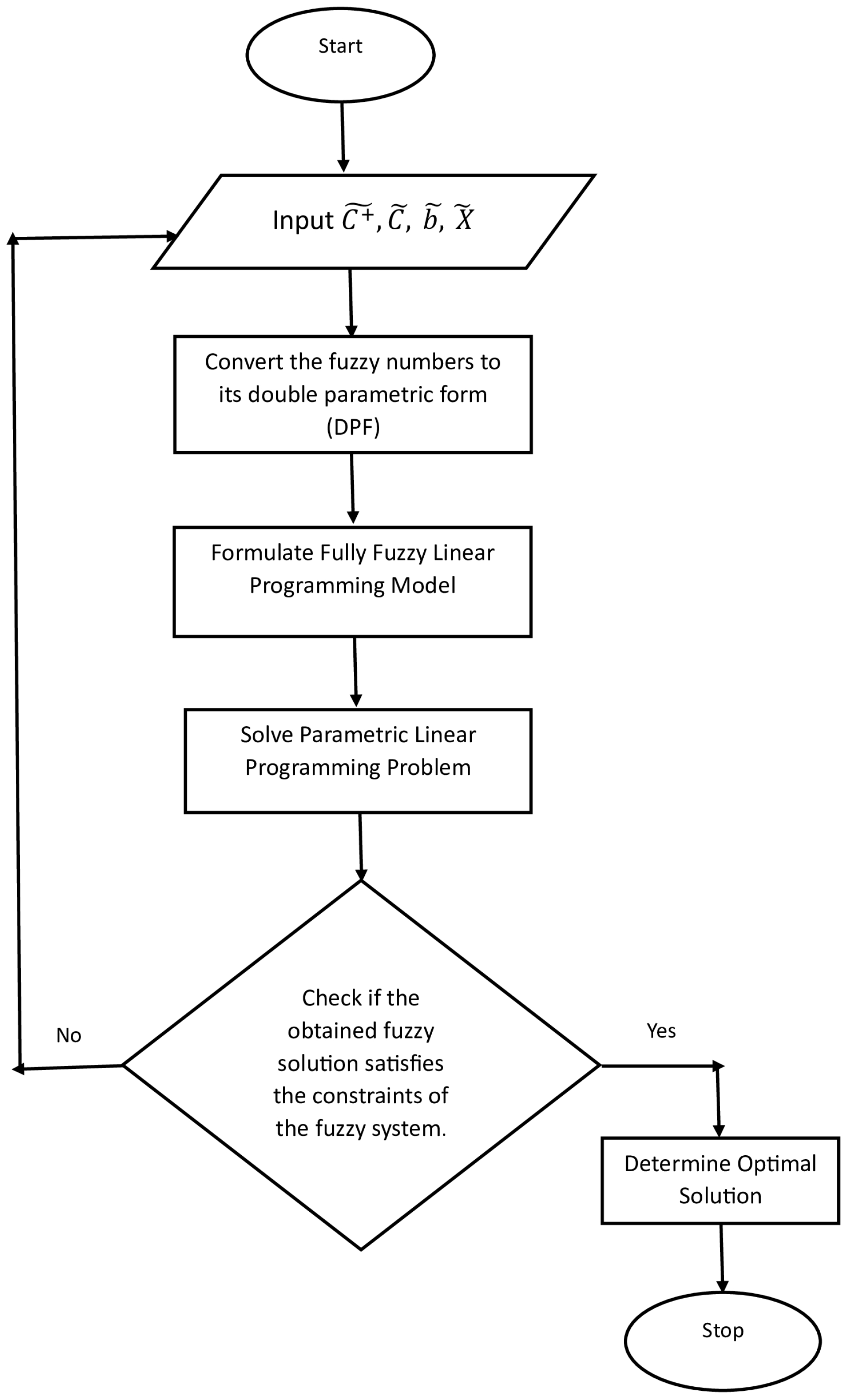Section 4 introduces the new method, accompanied by a flowchart in Figure 1 illustrating the approach. 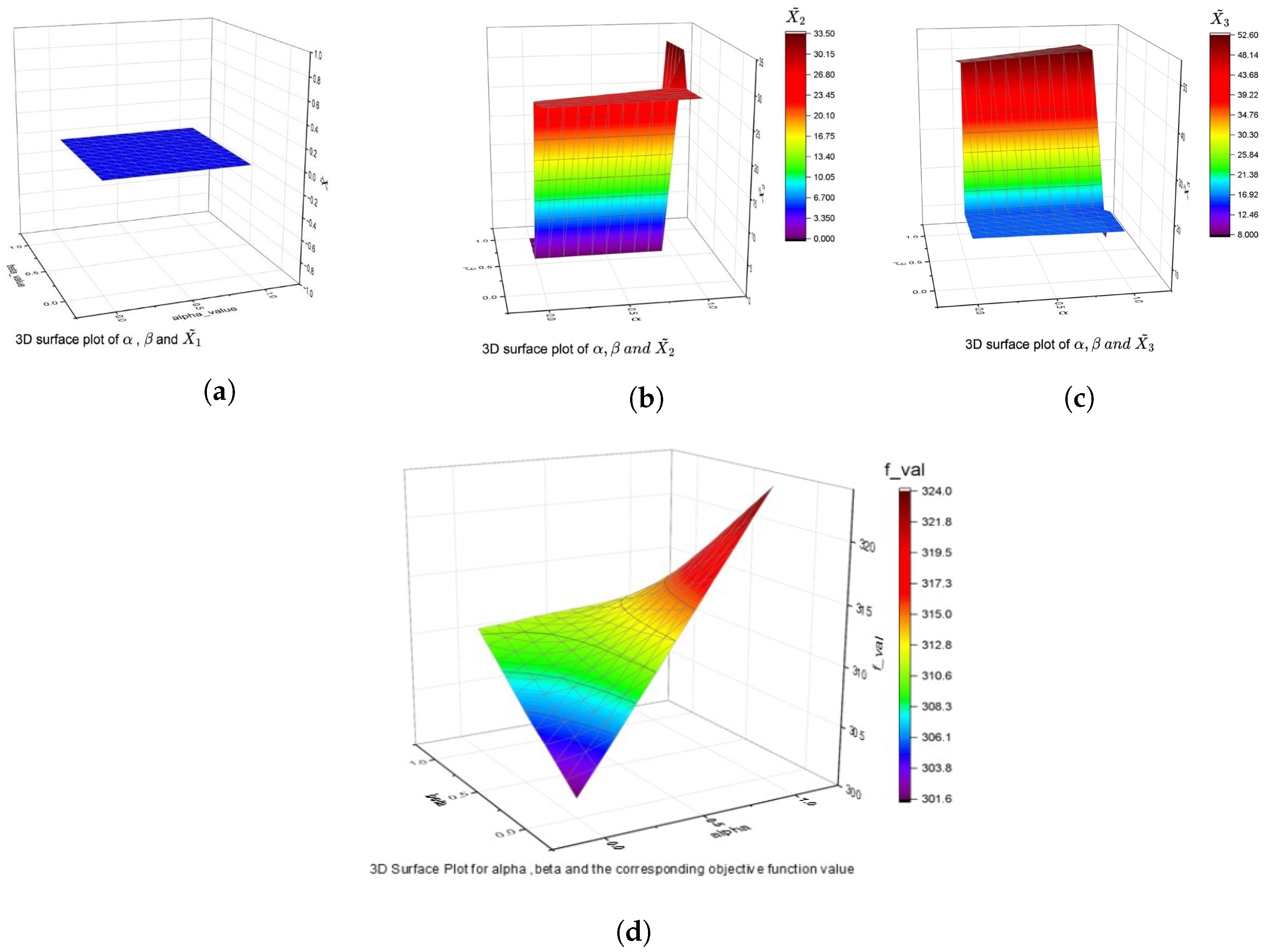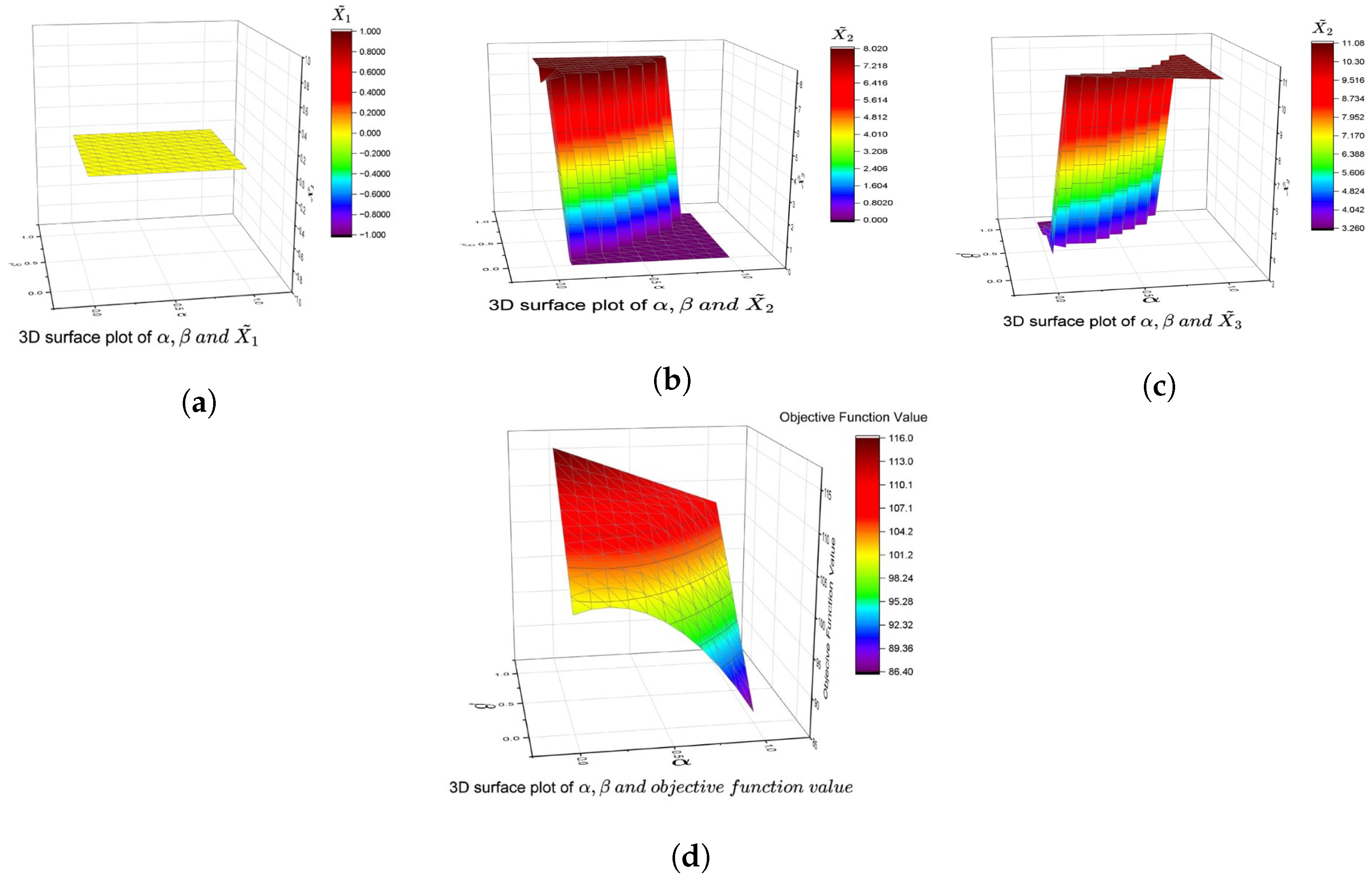Section 5 presents numerical examples to demonstrate the proposed method, along with a comparison of results and a detailed discussion of the figures obtained. The computational complexity of the proposed method and its comparison with other methods are included in Section 6. A summary and the conclusions are mentioned in Section 7. This section also includes future work.

Figure 1. Flowchart of the proposed method.

The abbreviations used in this paper and their definitions are listed in Table 1 to enhance clarity and facilitate better understanding of this paper.

Table 1. Table of abbreviations.

Abbreviations	Definitions
MOLP	Multi-Objective Linear Programming
FFLP	Fully Fuzzy Linear Programming
FSLEs	Fuzzy System of Linear Equations
FLP	Fuzzy Linear Programming
TFN	Triangular Fuzzy Number
TFNs	Triangular Fuzzy Numbers
FFSLEs	Fully Fuzzy System of Linear Equations
CLP	Crisp Linear Programming
DPF	Double Parametric Form
SPF	Single Parametric Form
$so{l}^n$	Solution
$eq{u}^n$	Equation

2. Preliminaries

Definition 1

([36]). A fuzzy set $\tilde{C}$ in a universal set X is denoted by its membership function ${\mu }_{\tilde{C}}$, which is defined as

$${\mu }_{\tilde{C}}:X⟶[0,1]$$

For each element $x\in X$, ${\mu }_{\tilde{C}}(x)$ represents the membership degree of $x\in \tilde{C}$.

Definition 2

([37]). A fuzzy set $\tilde{C}$ with the membership function ${\mu }_{\tilde{C}}:X⟶[0,1]$ becomes a fuzzy number if it satisfies the following conditions:

(i) 

Normalized:

$$\exists x_0\in Xsuchthat{\mu }_{\tilde{C}}(x_0)=1$$

This means that the fuzzy set reaches a membership value of 1 with at least one point $x_0$.

(ii) 

Convex:

$${\mu }_{\tilde{C}}(\eta x_0+(1-\eta )x_1)\ge min({\mu }_{\tilde{C}}(x_0),{\mu }_{\tilde{C}}(x_1))\forall x_0,x_1\in X,\eta \in [0,1]$$

(iii) 

Upper Semi-Continuity:

$$\underset{x\to x_0}{lim}sup{\mu }_{\tilde{C}}(x)\le {\mu }_{\tilde{C}}(x_0)$$

(iv) 

Compact Core: The core of $\tilde{C}$ is defined as

$$\overline{\{x\in \mathbb{R}:{\mu }_{\tilde{C}}(x)>0\}}$$

which must be a compact set in $\mathbb{R}$. This means that the core is bounded and closed in $\mathbb{R}$.

Definition 3

([12]). TFN denoted as $\tilde{W}=(w_1,w_2,w_3)$, is characterized by a membership function ${\mu }_{\tilde{W}}$, defined as follows:

$${\mu }_{\tilde{W}}(x)=\left\{\begin{array}{cc}0,\hfill & x\le w_1\hfill \\ {\displaystyle \frac{x-w_1}{w_2-w_1}},\hfill & w_1\le x\le w_2\hfill \\ {\displaystyle \frac{w_3-x}{w_3-w_2}},\hfill & w_2\le x\le w_3\hfill \\ 0,\hfill & x\ge w_3\hfill \end{array}\right.$$

TFN is classified further based on its positivity:

• A positive TFN satisfies ${\mu }_{\tilde{W}}(x)=0$ for all $x\le 0$, meaning it has no support in the negative range and is denoted as $\tilde{W}>0$.
• A non-negative TFN satisfies ${\mu }_{\tilde{W}}(x)=0$ for all $x<0$, meaning it has no support strictly in the negative range and is denoted as $\tilde{W}\ge 0$.

Definition 4

([38]). Let ${[\tilde{W}]}_{\alpha }$ be the α-levels of the fuzzy number $\tilde{W}$. Then, ${[\tilde{W}]}_{\alpha }$ can be defined as

$${[\tilde{W}]}_{\alpha }=\overline{\{x\in \mathbb{R}:{\mu }_{\tilde{W}}(x)>\alpha \}}where0<\alpha \le 1$$

Now, a more practical interval-based representation of the $\alpha$-level set ${[\tilde{W}]}_{\alpha }=[\underline{\mathrm{w}}(\alpha ),\overline{w}(\alpha )]$ for all $0\le \alpha \le 1$ [39] can be derived from Definition 4. Here, $\underline{\mathrm{w}}(\alpha )$ is the left endpoint of the interval, i.e., the smallest $x\in \mathbb{R}$ such that ${\mu }_{\tilde{W}}(x)>\alpha$, and $\overline{w}(\alpha )$ is the right endpoint of the interval, i.e., the largest $x\in \mathbb{R}$ such that ${\mu }_{\tilde{W}}(x)>\alpha$.

Lemma 1 provides the if and only if conditions for a collection of intervals $[\underline{\mathrm{w}}(\alpha ),\overline{w}(\alpha )]$, where $\alpha \in [0,1]$, to serve as the $\alpha$-levels of a fuzzy number belonging to the set $\mathbb{F}$ of all fuzzy numbers. The conditions in Lemma 1 are significant because they establish a solid mathematical foundation for working with fuzzy numbers, ensuring that their $\alpha$-levels accurately represent the fuzzy numbers and can be reliably used in practical and theoretical applications.

Lemma 1

([40]). Suppose that $\{[\underline{w}(\alpha ),\overline{w}(\alpha )],\forall \alpha \in [0,1]\}$ is a given collection of non-empty sets in $\mathbb{R}$. If the following conditions hold:

1. 

$\forall \alpha \in [0,1]$, $[\underline{w}(\alpha ),\overline{w}(\alpha )]$ is a bounded closed interval.

2. 

$\forall 0\le {\alpha }_1\le {\eta }_1\le 1$, $[\underline{w}({\alpha }_1),\overline{w}({\alpha }_1)]\supseteq [\underline{w}({\eta }_1),\overline{w}({\eta }_1)].$

3. 

For ${\alpha }_k$ to be a non-decreasing sequence in $[0,1]$ converging to α, it satisfies

$$[\underset{k\to \infty }{lim}\underline{w}({\alpha }_k),\underset{k\to \infty }{lim}\overline{w}({\alpha }_k)]=[\underline{w}(\alpha ),\overline{w}(\alpha )]$$

Then, the α-levels of $\tilde{W}$ in $\mathbb{F}$ are represented by the family $[\underline{w}(\alpha ),\overline{w}(\alpha )]$ and vice versa. Here, $\tilde{W}$ is a fuzzy number.

Remark 1

([41]). The first condition of Lemma 1 implies the boundedness of $\underline{w}$ and $\overline{w}$ and for each $\alpha \in [0,1]$, $\underline{w}(\alpha )\le \overline{w}(\alpha )$.

Remark 2

([41]). The non-decreasingness of $\underline{w}$ over $[0,1]$ and non-increasingness of $\overline{w}$ over $[0,1]$ can be derived from the second condition of Lemma 1.

Remark 3

([41]). The left-continuity of $\underline{w}$ and $\overline{w}$ over $[0,1]$ is represented by the third condition of Lemma 1.

Definition 5

([12]). For a TFN $\tilde{W}=(w_1,w_2,w_3)$, the SPF is denoted as $[\underline{w}(\alpha ),\overline{w}(\alpha )]$ and defined as $[\underline{w}(\alpha ),\overline{w}(\alpha )]=[(w_2-w_1)\alpha +w_1,w_3-(w_3-w_2)\alpha ]$, where $\alpha \in [0,1]$.

Definition 6

([12]). The DPF of a TFN $\tilde{W}$ is denoted by $\tilde{W}(\alpha ,\beta )$ and is defined as $\tilde{W}(\alpha ,\beta )=\beta (\overline{w}(\alpha )-\underline{w}(\alpha ))+\underline{w}(\alpha )$, where $\alpha ,\beta \in [0,1]$. Here, $\overline{w}(\alpha )$ and $\underline{w}(\alpha )$ comes from Definition 5.

Remark 4.

The parametric form $[\underline{w}(\alpha ),\overline{w}(\alpha )]$ is derived from the membership function ${\mu }_{\tilde{W}}(x)$ by considering the α-cut of the fuzzy number. The $\tilde{W}(\alpha )$ is the set of all x such that ${\mu }_{\tilde{W}}(x)\ge \alpha$, and it forms the basis for defining the interval $\left[\underline{w}(\alpha ),\overline{w}(\alpha )\right]$. This clarification is necessary to bridge the gap between the initial definition of a TFN and the operations performed on fuzzy numbers in the interval form.

Definition 7

([12]). Let $\widetilde{W_1}$ and $\widetilde{W_2}$ be any arbitrary fuzzy number and l be a scalar. Using the SPF, the fuzzy numbers may be converted into an interval. The interval form of $\widetilde{W_1}$ and $\widetilde{W_2}$ is defined as $\widetilde{W_1}=[\underline{w_1}(\alpha ),\overline{w_1}(\alpha )]$ and $\widetilde{W_2}=[\underline{w_2}(\alpha ),\overline{w_2}(\alpha )]$. The interval-based fuzzy arithmetic is as follows:

1. 

$\widetilde{W_1}=\widetilde{W_2}$ iff $\underline{w_1}(\alpha )=\underline{w_2}(\alpha )$ and $\overline{w_1}(\alpha )=\overline{w_2}(\alpha )$.

2. 

$\widetilde{W_1}\oplus \widetilde{W_2}=[\underline{w_1}(\alpha )+\underline{w_2}(\alpha ),\overline{w_1}(\alpha )+\overline{w_2}(\alpha )]$.

3. 

$\widetilde{W_1}\ominus \widetilde{W_2}=[\underline{w_1}(\alpha )-\overline{w_2}(\alpha ),\overline{w_1}(\alpha )-\underline{w_2}(\alpha )]$.

4. 

$\widetilde{W_1}\otimes \widetilde{W_2}=[min(T),max(T)],$

$$\begin{array}{cc}\hfill whereT& =[\underline{w_1}(\alpha )\times \underline{w_2}(\alpha ),\underline{w_1}(\alpha )\times \overline{w_2}(\alpha ),\hfill \\ \hfill & \overline{w_1}(\alpha )\times \underline{w_2}(\alpha ),\overline{w_1}(\alpha )\times \overline{w_2}(\alpha )].\hfill \end{array}$$

5. 

$l\odot \tilde{W}=\left\{\begin{array}{cc}[l\overline{w}(\alpha ),l\underline{w}(\alpha )],\hfill & l<0\hfill \\ \underline{w}(\alpha ),l\overline{w}(\alpha )],\hfill & l\ge 0\hfill \end{array}\right.$.

3. FFLP Problem

In situations involving uncertainty and imprecision, the parameters in linear programming problems can be modeled using fuzzy numbers. FFLP problems can be expressed in the following way:

$$\begin{array}{cc}\hfill Max(orMin)& \widetilde{C^{+}}\otimes \tilde{X}\hfill \\ \hfill subjectto& \tilde{C}\otimes \tilde{X}\le ,=,\ge \tilde{b}\hfill \end{array}$$

(1)

where $\widetilde{C^{+}},\tilde{X},\tilde{C},$ and $\tilde{b}$ are equal to ${[{\tilde{c}}_j]}_{1\times n},{[{\tilde{x}}_j]}_{n\times 1},{[{\tilde{a}}_{ij}]}_{m\times n},$ and ${[{\tilde{b}}_i]}_{m\times 1}$, respectively. ${\tilde{a}}_{ij},{\tilde{b}}_i,{\tilde{c}}_j\in F(\mathbb{R})$; and ${\tilde{x}}_j$ is a fuzzy number which is non-negative. m and n represent the number of constraints and variables which are fuzzy, respectively.

Theorem 1.

Let $\tilde{C}(\alpha ,\beta )$ be a fuzzy coefficient matrix, $\tilde{b}(\alpha ,\beta )$ be a fuzzy right-hand-side vector, and $\tilde{X}(\alpha ,\beta )$ represent the decision variables, all in double parametric form. If the following conditions hold:

(i) 

$\tilde{C}(\alpha ,\beta )\ge 0,$ meaning that all the fuzzy matrix are non-negative.

(ii) 

$\tilde{b}(\alpha ,\beta )\ge 0,$ meaning that all the elements of the fuzzy right-hand-side vector are non-negative.

(iii) 

$\tilde{C}(\alpha ,\beta )$ corresponds to a permutation matrix or a diagonally dominant fuzzy matrix.

Then, there exists a non-negative fuzzy solution $\tilde{X}(\alpha ,\beta )\ge 0$ to the fully fuzzy linear programming problem given by

$$\begin{array}{cc}\hfill Max(orMin)& \widetilde{C^{+}}(\alpha ,\beta )\tilde{X}(\alpha ,\beta )\hfill \\ \hfill subjectto& \tilde{C}(\alpha ,\beta )\tilde{X}(\alpha ,\beta )\le ,=,\ge \tilde{b}(\alpha ,\beta )\hfill \\ \hfill and& \tilde{X}(\alpha ,\beta )\ge 0\hfill \end{array}$$

(2)

Proof. 

The proof follows similarly to the case for fully fuzzy linear systems [12]. Given that $\tilde{C}(\alpha ,\beta )\ge 0,$ and is a permutation matrix, it guarantees that $\tilde{C}{(\alpha ,\beta )}^{-1}$ exists and is non-negative (by the theory of non-negative matrices). Therefore, solving the following system:

$$\tilde{X}(\alpha ,\beta )\le ,=,\ge \tilde{C}{(\alpha ,\beta )}^{-1}\tilde{b}(\alpha ,\beta )$$

yields a non-negative fuzzy solution $\tilde{X}(\alpha ,\beta )\ge 0$. Thus, the theorem has been proven. □

3.1. The Significance of $\alpha$ and $\beta$

• $\alpha$ (Level of Membership): $\alpha$ is a parameter that represents the degree of membership or confidence level in the context of fuzzy numbers. It ranges from 0 to 1, which involve the following:

  −

  $\alpha =1$ represents the core of the fuzzy number, where the membership function is at its maximum value 1;

  −

  $\alpha =0$ represents the outer boundary of the fuzzy number, where the membership function is zero.

• $\beta$ (Parametric Coefficient):

  −

  $\beta$ is a parameter used to express the degree of uncertainty or scaling factor in the parametric form of fuzzy numbers. It also ranges from 0 to 1, and it is used to scale or adjust the fuzzy numbers according to different levels of uncertainty.

  −

  $\beta$ helps in transforming the fuzzy number into a more manageable form by expressing it as a combination of linear functions of $\alpha$. This makes it easier to perform mathematical operations on fuzzy numbers by converting them into a parametric form.

3.2. Basic Steps to Establish This Research Work

The research work is established through the following basic steps:

• Problem Identification: Identify the limitations in existing methods for solving FFLP problems, particularly in handling fuzziness effectively.
• Formulation: Develop a mathematical formulation using TFNs to represent the FFLP problem.
• Method Development: Introduce a novel approach by converting fuzzy numbers into parametric form and systematically addressing different constraint types.
• Iterative Evaluation: Implement an iterative process to explore various scenarios, optimizing the solution based on the objective function.
• Validation: Compare the proposed method with existing techniques to demonstrate its effectiveness and computational feasibility.

These steps provide a structured approach to addressing the complexities of FFLP problems in the research.

4. Proposed Method

Mathematically, the FFLP problem can be represented by

$$\begin{array}{cc}\hfill Max(orMin)& \widetilde{C^{+}}\otimes \tilde{X}\hfill \\ \hfill subjectto& \tilde{C}\otimes \tilde{X}\le ,=,\ge \tilde{b}\hfill \end{array}$$

(3)

$\tilde{X}$ is a non-negative fuzzy number, where $\widetilde{C^{+}}={[{\tilde{c}}_j]}_{1\times n},\tilde{X}={[{\tilde{x}}_j]}_{n\times 1},\tilde{C}={[{\tilde{a}}_{ij}]}_{m\times n},$ $\tilde{b}={[{\tilde{b}}_i]}_{m\times 1}$ and ${\tilde{a}}_{ij},{\tilde{b}}_i,{\tilde{c}}_j\in F(\mathbb{R})$. Here, $F(\mathbb{R})$ is the set of fuzzy sets on real numbers.

The proposed method can be applied step by step in the following way:

Step 1: Substitute ${[{\tilde{c}}_j]}_{1\times n},{[{\tilde{x}}_j]}_{n\times 1},{[{\tilde{a}}_{ij}]}_{m\times n},{[{\tilde{b}}_i]}_{m\times 1}$ in place of $\widetilde{C^{+}},\tilde{X},\tilde{C},\tilde{b}$, respectively; then, Equation (3) takes the form

$$\begin{array}{cc}\hfill Max(orMin)& \sum _{j=1}^n{\tilde{c}}_j\otimes {\tilde{x}}_j\hfill \\ \hfill subjectto& \sum _{j=1}^n{\tilde{a}}_{ij}\otimes {\tilde{x}}_j\le ,=,\ge {\tilde{b}}_i\hfill \end{array}$$

(4)

where ${\tilde{x}}_j$ is a non-negative fuzzy number and ${\tilde{a}}_{ij},{\tilde{b}}_i,{\tilde{c}}_j$ are any type of TFNs. Depending on the nature of the constraints, the constraints can be classified as

(i)

Equality Constraints:

$$\sum _{j=1}^n{\tilde{a}}_{ij}\otimes {\tilde{x}}_j={\tilde{b}}_i$$

(ii)

Inequality Constraints:

$$\sum _{j=1}^n{\tilde{a}}_{ij}\otimes {\tilde{x}}_j\ne {\tilde{b}}_i$$

Here, the following two cases may arise:

• Case 1: ${\sum }_{j=1}^n{\tilde{a}}_{q_j}\otimes {\tilde{x}}_j\le {\tilde{b}}_p$ for some $p\in \{1,2,\dots ,m\}$
• Case 2: ${\sum }_{j=1}^n{\tilde{a}}_{q_j}\otimes {\tilde{x}}_j\ge {\tilde{b}}_q$ for some $q\in \{1,2,\dots ,m\}$

Step 2: Then, the FFLP problem can be written as

$$\begin{array}{cc}\hfill Max(orMin)& \sum _{j=1}^n(p_j,q_j,r_j)\otimes (x_j,y_j,z_j)\hfill \\ \hfill subjectto& \\ \hfill & \sum _{j=1}^n(a_{p_j},b_{p_j},c_{p_j})\otimes (x_j,y_j,z_j)\le (t_p,u_p,v_p)\hfill \\ \hfill & \sum _{j=1}^n(a_{q_j},b_{q_j},c_{q_j})\otimes (x_j,y_j,z_j)\ge (t_q,u_q,v_q)\hfill \\ \hfill & \sum _{j=1}^n(a_{r_j},b_{r_j},c_{r_j})\otimes (x_j,y_j,z_j)=(t_r,u_r,v_r)\hfill \end{array}$$

(5)

where $(x_j,y_j,z_j)$ is a non-negative fuzzy number and $(p_j,q_j,r_j),$ $(a_{p_j},b_{p_j},c_{p_j}),(a_{q_j},b_{q_j},c_{q_j})$, $(a_{r_j},b_{r_j},c_{r_j})$, $(t_p,u_p,v_p),(t_q,u_q,v_q),(t_r,u_r,v_r)$ are any type of TFNs.

Step 3: After using the DPF, the FFLP problem can take the form

$$\begin{array}{cc}\hfill Max(orMin)& \sum _{j=1}^n[\beta \{(r_j-p_j)+(p_j-r_j)\alpha \}+(q_j-p_j)\alpha +p_j]\times \hfill \\ \hfill & [\beta \{(z_j-x_j)+(x_j-z_j)\alpha \}+(y_j-x_j)\alpha +x_j]\hfill \\ \hfill subjectto& \sum _{j=1}^n[\beta \{(c_{p_j}-a_{p_j})+(a_{p_j}-c_{p_j})\alpha \}+(b_{p_j}-a_{p_j})\alpha +a_{p_j}]\times \hfill \\ \hfill & [\beta \{(z_j-x_j)+(x_j-z_j)\alpha \}+(y_j-x_j)\alpha +x_j]\hfill \\ \hfill & \le \beta \{(v_p-t_p)+(t_p-v_p)\alpha \}+(u_p-t_p)\alpha +t_p\hfill \\ \hfill & \sum _{j=1}^n[\beta \{(c_{q_j}-a_{q_j})+(a_{q_j}-c_{q_j})\alpha \}+(b_{q_j}-a_{q_j})\alpha +a_{q_j}]\times \hfill \\ \hfill & [\beta \{(z_j-x_j)+(x_j-z_j)\alpha \}+(y_j-x_j)\alpha +x_j]\hfill \\ \hfill & \ge \beta \{(v_q-t_q)+(t_q-v_q)\alpha \}+(u_q-t_q)\alpha +t_q\hfill \\ \hfill & \sum _{j=1}^n[\beta \{(c_{r_j}-a_{r_j})+(a_{r_j}-c_{r_j})\alpha \}+(b_{r_j}-a_{r_j})\alpha +a_{r_j}]\times \hfill \\ \hfill & [\beta \{(z_j-x_j)+(x_j-z_j)\alpha \}+(y_j-x_j)\alpha +x_j]\hfill \\ \hfill & =\beta \{(v_r-t_r)+(t_r-v_r)\alpha \}+(u_r-t_r)\alpha +t_r\hfill \end{array}$$

(6)

$$\begin{array}{cc}\hfill Max(orMin){\beta }^2& \sum _{j=1}^n(r_j-p_j)(z_j-x_j)+\alpha {\beta }^2\sum _{j=1}^n(r_j-p_j)(x_j-z_j)+(p_j-r_j)(z_j-x_j)+\hfill \\ \hfill {\alpha }^2{\beta }^2& \sum _{j=1}^n(p_j-r_j)(x_j-z_j)+{\alpha }^2\beta \sum _{j=1}^n(p_j-r_j)(y_j-x_j)+(q_j-p_j)(x_j-z_j)+\hfill \\ \hfill \alpha \beta & \sum _{j=1}^n(r_j-p_j)(y_j-x_j)+(p_j-r_j)x_j+(q_j-p_j)(z_j-x_j)+(x_j-z_j)p_j+\hfill \\ \hfill \beta & \sum _{j=1}^n(r_j-p_j)x_j+(z_j-x_j)p_j+\alpha \sum _{j=1}^n(q_j-p_j)x_j+(y_j-x_j)p_j+\hfill \\ \hfill {\alpha }^2& \sum _{j=1}^n(q_j-p_j)(y_j-x_j)+\sum _{j=1}^n{p}_j{x}_j\hfill \\ \hfill subjectto{\beta }^2& \sum _{j=1}^n(c_{p_j}-a_{p_j})(z_j-x_j)+\alpha {\beta }^2\sum _{j=1}^n(c_{p_j}-a_{p_j})(x_j-z_j)+(a_{p_j}-c_{p_j})(z_j-x_j)+\hfill \\ \hfill {\alpha }^2{\beta }^2& \sum _{j=1}^n(a_{p_j}-c_{p_j})(x_j-z_j)+{\alpha }^2\beta \sum _{j=1}^n(a_{p_j}-c_{p_j})(y_j-x_j)+(b_{p_j}-a_{p_j})(x_j-z_j)+\hfill \\ \hfill \alpha \beta & \sum _{j=1}^n(c_{p_j}-a_{p_j})(y_j-x_j)+(a_{p_j}-c_{p_j})x_j+(b_{p_j}-a_{p_j})(z_j-x_j)+(x_j-z_j)a_{p_j}+\hfill \\ \hfill \beta & \sum _{j=1}^n(c_{p_j}-a_{p_j})x_j+(z_j-x_j)a_{p_j}+\alpha \sum _{j=1}^n(b_{p_j}-a_{p_j})x_j+(y_j-x_j)a_{p_j}+\hfill \\ \hfill {\alpha }^2& \sum _{j=1}^n(b_{p_j}-a_{p_j})(y_j-x_j)+\sum _{j=1}^n{a}_{p_j}{x}_j\hfill \\ \hfill & \le \beta \{(v_p-t_p)+(t_p-v_p)\alpha \}+(u_p-t_p)\alpha +t_p\hfill \\ \hfill {\beta }^2& \sum _{j=1}^n(c_{q_j}-a_{q_j})(z_j-x_j)+\alpha {\beta }^2\sum _{j=1}^n(c_{q_j}-a_{q_j})(x_j-z_j)+(a_{q_j}-c_{q_j})(z_j-x_j)+\hfill \\ \hfill {\alpha }^2{\beta }^2& \sum _{j=1}^n(a_{q_j}-c_{q_j})(x_j-z_j)+{\alpha }^2\beta \sum _{j=1}^n(a_{q_j}-c_{q_j})(y_j-x_j)+(b_{q_j}-a_{q_j})(x_j-z_j)+\hfill \\ \hfill \alpha \beta & \sum _{j=1}^n(c_{q_j}-a_{q_j})(y_j-x_j)+(a_{q_j}-c_{q_j})x_j+(b_{q_j}-a_{q_j})(z_j-x_j)+(x_j-z_j)a_{q_j}+\hfill \\ \hfill \beta & \sum _{j=1}^n(c_{q_j}-a_{q_j})x_j+(z_j-x_j)a_{q_j}+\alpha \sum _{j=1}^n(b_{q_j}-a_{q_j})x_j+(y_j-x_j)a_{q_j}+\hfill \\ \hfill {\alpha }^2& \sum _{j=1}^n(b_{q_j}-a_{q_j})(y_j-x_j)+\sum _{j=1}^n{a}_{q_j}{x}_j\hfill \\ \hfill & \ge \beta \{(v_q-t_q)+(t_q-v_q)\alpha \}+(u_q-t_q)\alpha +t_q\hfill \end{array}$$

$$\begin{array}{cc}\hfill {\beta }^2& \sum _{j=1}^n(c_{r_j}-a_{r_j})(z_j-x_j)+\alpha {\beta }^2\sum _{j=1}^n(c_{r_j}-a_{r_j})(x_j-z_j)+(a_{r_j}-c_{r_j})(z_j-x_j)+\hfill \\ \hfill {\alpha }^2{\beta }^2& \sum _{j=1}^n(a_{r_j}-c_{r_j})(x_j-z_j)+{\alpha }^2\beta \sum _{j=1}^n(a_{r_j}-c_{r_j})(y_j-x_j)+(b_{r_j}-a_{r_j})(x_j-z_j)+\hfill \\ \hfill \alpha \beta & \sum _{j=1}^n(c_{r_j}-a_{r_j})(y_j-x_j)+(a_{r_j}-c_{r_j})x_j+(b_{r_j}-a_{r_j})(z_j-x_j)+(x_j-z_j)a_{r_j}+\hfill \\ \hfill \beta & \sum _{j=1}^n(c_{r_j}-a_{r_j})x_j+(z_j-x_j)a_{r_j}+\alpha \sum _{j=1}^n(b_{r_j}-a_{r_j})x_j+(y_j-x_j)a_{r_j}+\hfill \\ \hfill {\alpha }^2& \sum _{j=1}^n(b_{r_j}-a_{r_j})(y_j-x_j)+\sum _{j=1}^n{a}_{r_j}{x}_j\hfill \\ \hfill & =\beta \{(v_r-t_r)+(t_r-v_r)\alpha \}+(u_r-t_r)\alpha +t_r\hfill \end{array}$$

(7)

Step 4: Solve the DPF of FFLP problem in Equation (7) for different combinations of $\alpha$ and $\beta$ within the range $[0,1]$ to find the corresponding solutions.

Step 5: Determine for which pair, $(\alpha ,\beta )$ or $x_j,y_j,z_j$, is the $so{l}^n$ optimal.

Flowchart of the Proposed Method

The flowchart of the proposed method is provided below.

5. Example

5.1. Product Mix Problem

As outlined in [15], the product mix problem involves a company that manufactures three products—$P_1$, $P_2$ and $P_3$—which must be processed through three departments: $D_1$, $D_2$, and $D_3$. Table 2 provides the estimated time (in hours) that each product spends in each department.

Table 2. Product Mix Problem: Estimated times for product $P_i$ is in department $D_j$.

Product	Department
	${\mathit{D}}_{\mathbf{1}}$	${\mathit{D}}_{\mathbf{2}}$	${\mathit{D}}_{\mathbf{3}}$
$P_1$	6	12	2
$P_2$	8	8	4
$P_3$	3	6	1

The company’s goal is to maximize its revenue by determining the optimal number of units to produce for each product on a weekly basis. According to [15], the maximum available processing hours per week are $288 \mathrm{h}$, $312 \mathrm{h}$, and $124 \mathrm{h}$ for $D_1$, $D_2$, and $D_3$, respectively. Additionally, the average selling prices for $P_1$, $P_2$, and $P_3$ are $ 6, $ 8, and $ 6 respectively.

In the presence of uncertainty, the problem will be modeled as an FFLP problem. Each given value will be substituted with a TFN (Table 3) where the peak of the fuzzy number is at the number given. Therefore, the FFLP problem can be written as follows:

$$\begin{array}{cc}\hfill & Max\tilde{Z}=\left[\begin{array}{ccc}(5.8,6,6.2)& (7.5,8,8.5)& (5.6,6,6.4)\end{array}\right]\otimes \left[\begin{array}{c}{\tilde{X}}_i\end{array}\right]\hfill \end{array}$$

$$\begin{array}{cc}\hfill & Subjectto:\left[\begin{array}{ccc}(5.6,6,6.4)& (7.5,8,8.5)& (2.8,3,3.2)\\ (11.4,12,12.6)& (7.6,8,8.4)& (5.7,6,6.3)\\ (1.8,2,2.2)& (3.8,4,4.2)& (0.9,1,1.1)\end{array}\right]\otimes \left[\begin{array}{c}{\tilde{X}}_i\end{array}\right]\le \left[\begin{array}{c}(283,288,293)\\ (306,312,318)\\ (121,124,127)\end{array}\right]\hfill \end{array}$$

(8)

where ${\tilde{X}}_i\ge 0\mathrm{and}{\tilde{X}}_i=(x_i,y_i,z_i),i=1,2,3$.

Table 3. Product Mix Problem: Fuzzy representation of the estimated times that product $P_i$ is in department $D_j$.

Product	Department
	${\mathit{D}}_{\mathbf{1}}$	${\mathit{D}}_{\mathbf{2}}$	${\mathit{D}}_{\mathbf{3}}$
$P_1$	$(5.6,6,6.4)$	$(11.4,12,12.6)$	$(1.8,2,2.2)$
$P_2$	$(7.5,8,8.5)$	$(7.6,8,8.4)$	$(3.8,4,4.2)$
$P_3$	$(2.8,3,3.2)$	$(5.7,6,6.3)$	$(0.9,1,1.1)$

Using the DPF, the above problem can be written in following way:

$$\begin{array}{cc}\hfill & \begin{array}{cc}\hfill Max& {\beta }^2(0.4z_1-0.4x_1+z_2-x_2+0.8z_3-0.8x_3)+\hfill \\ \hfill & \alpha {\beta }^2(0.8x_1-0.8z_1+2x_2-2z_2+1.6x_3-1.6z_3)+\hfill \\ \hfill & {\alpha }^2{\beta }^2(0.4z_1-0.4x_1+z_2-x_2+0.8z_3-0.8x_3)+\hfill \\ \hfill & \alpha \beta (4.8x_1+0.4y_1-5.6z_1+5x_2+y_2-7x_2+3.6x_3+0.8y_3-5.2z_3)+\hfill \\ \hfill & \alpha (-5.6x_1+5.8y_1-7x_2+7.5y_2-5.2x_3+5.6y_3)+\hfill \\ \hfill & \beta (-5.4x_1+5.8z_1-6.5x_2+7.5z_2-4.8x_3+5.6z_3)+\hfill \\ \hfill & {\alpha }^2\beta (0.6x_1-0.4y_1-0.2z_1+1.5x_2-y_2-0.5z_2+1.2x_3-0.8y_3-0.4z_3)+\hfill \\ \hfill & {\alpha }^2(-0.2x_1+0.2y_1-0.5x_2+0.5y_2-0.4x_3+0.4y_3)+5.8x_1+7.5x_2+5.6x_3\hfill \\ \hfill subjectto& \hfill \\ \hfill & {\beta }^2(0.8z_1-0.8x_1+z_2-x_2+0.4z_3-0.4x_3)+\hfill \\ \hfill & \alpha {\beta }^2(1.6x_1-1.6z_1+2x_2-2z_2+0.8x_3-0.8z_3)+\hfill \\ \hfill & {\alpha }^2{\beta }^2(0.8z_1-0.8x_1+z_2-x_2+0.4z_3-0.4x_3)+\hfill \\ \hfill & \alpha \beta (3.6x_1+0.8y_1-5.2z_1+5x_2+y_2-7z_2+1.8x_3+0.4y_3-2.6z_3)+\hfill \\ \hfill & \alpha (-5.2x_1+5.6y_1-7x_2+7.5y_2-2.6x_3+2.8y_3)+\hfill \\ \hfill & \beta (-4.8x_1+5.6z_1-6.5x_2+7.5z_2-2.4x_3+2.8z_3)+\hfill \\ \hfill & {\alpha }^2\beta (1.2x_1-0.8y_1-0.4z_1+1.5x_2-y_2-0.5z_2+0.6x_3-0.4y_3-0.2z_3)+\hfill \\ \hfill & {\alpha }^2(-0.4x_1+0.4y_1-0.5x_2+0.5y_2-0.2x_3+0.2y_3)+\hfill \\ \hfill & 5.6x_1+7.5x_2+2.8x_3\le 10\beta +5\alpha -10\alpha \beta +283\hfill \\ \\ \hfill & {\beta }^2(1.2z_1-1.2x_1+0.8z_2-0.8x_2+0.6z_3-0.6x_3)+\hfill \\ \hfill & \alpha {\beta }^2(2.4x_1-2.4z_1+1.6x_2-1.6z_2+1.2x_3-1.2z_3)+\hfill \\ \hfill & {\alpha }^2{\beta }^2(1.2z_1-1.2x_1+0.8z_2-0.8x_2+0.6z_3-0.6x_3)+\hfill \\ \hfill & \alpha \beta (8.4x_1+1.2y_1-10.8z_1+5.6x_2+0.8y_2-7.2z_2+4.2x_3+0.6y_3-5.4z_3)+\hfill \\ \hfill & \alpha (-10.8x_1+11.4y_1-7.2x_2+7.6y_2-5.4x_3+5.7y_3)+\hfill \\ \hfill & \beta (-10.2x_1+11.4z_1-6.8x_2+7.6z_2-5.1x_3+5.7z_3)+\hfill \\ \hfill & {\alpha }^2\beta (1.8x_1-1.2y_1-0.6z_1+1.2x_2-0.8y_2-0.4z_2+0.9x_3-0.6y_3-0.3z_3)+\hfill \\ \hfill & {\alpha }^2(-0.6x_1+0.6y_1-0.4x_2+0.4y_2-0.3x_3+0.3y_3)+\hfill \\ \hfill & 11.4x_1+7.6x_2+5.7x_3\le 12\beta +6\alpha -12\alpha \beta +306\hfill \\ \\ \hfill & {\beta }^2(0.4z_1-0.4x_1+0.4z_2-0.4x_2+0.2z_3-0.2x_3)+\hfill \\ \hfill & \alpha {\beta }^2(0.8x_1-0.8z_1+0.8x_2-0.8z_2+0.4x_3-0.4z_3)+\hfill \\ \hfill & {\alpha }^2{\beta }^2(0.4z_1-0.4x_1+0.4z_2-0.4x_2+0.2z_3-0.2x_3)+\hfill \\ \hfill & \alpha \beta (0.8x_1+0.4y_1-1.6z_1+2.8x_2+0.4y_2-3.6z_2+0.4x_3+0.2y_3-0.8z_3)+\hfill \\ \hfill & \alpha (-1.6x_1+1.8y_1-3.6x_2+3.8y_2-0.8x_3+0.9y_3)+\hfill \\ \hfill & \beta (-1.4x_1+0.2z_1-3.4x_2+3.8z_2-0.7x_3+0.9z_3)+\hfill \\ \hfill & {\alpha }^2\beta (0.6x_1-0.4y_1-0.2z_1+0.6x_2-0.4y_2-0.2z_2+0.3x_3-0.2y_3-0.1z_3)+\hfill \\ \hfill & {\alpha }^2(-0.2x_1+0.2y_1-0.2x_2+0.2y_2-0.1x_3+0.1y_3)+\hfill \\ \hfill & 1.8x_1+3.8x_2+0.9x_3\le 6\beta +3\alpha -6\alpha \beta +121\hfill \end{array}\hfill \end{array}$$

(9)

To overcome the limitations of the existing method, the example problem of the FFLP problem has been solved by the proposed method. The problem has previously been solved in [15]. The comparison results with the proposed method are tabulated in Table 4. In the proposed methodology, the FFLP problem turns into a parametric form, which can be solved in Python. Also, the 3D plots of the variables are shown in Figure 2, where Figure 2a–c present the 3D surface plots of $\alpha ,\beta$ vs. $\widetilde{X_1}$, $\alpha ,\beta$ vs. $\widetilde{X_2}$, and $\alpha ,\beta$ vs. $\widetilde{X_3}$ respectively, while Figure 2d represents the 3D surface plot of $\alpha ,\beta$ vs. the objective function value. Using the method proposed in Section 4, the solution is $\widetilde{X_1}=0$ (for $P_1$), $\widetilde{X_2}=28.5$ (for $P_2$), and $\widetilde{X_3}=16$ (for $P_3$) with the maximum objective function value 324.

Table 4. Product Mix Problem: Comparison of solution between the existing method and the proposed method.

Product	Buckley and Feuring [15]	Proposed Method
$P_1$	0	0
$P_2$	27	28.5
$P_3$	16	16
Max Z	312	324

Figure 2. Product Mix Problem: (a) 3D surface plot of $\alpha ,\beta \mathrm{and}\widetilde{X_1}$, (b) 3D surface plot of $\alpha ,\beta \mathrm{and}\widetilde{X_2}$, (c) 3D surface plot of $\alpha ,\beta \mathrm{and}\widetilde{X_3}$, (d) 3D surface plot of $\alpha ,\beta$ and corresponding objective function value.

Discussion of the Figures of Product Mix Problem

Figure 2 is described below in detail, along with descriptions of the axes, for a better understanding of the nature of the solution of the product mix problem using the proposed method:

(I)

Figure 2a

• Axes: The $x,y,$ and z axes correspond to the variables $\alpha ,\beta ,$ and $\widetilde{X_1}$, respectively.
• Interpretation: The flat surface at a particular value on the z axis indicates that changes in $\alpha$ and $\beta$ do not affect the value of $\widetilde{X_1}$. This could indicate a situation where $\widetilde{X_1}$ is a constant or invariant with respect to the other variables in the region under consideration.

(II)

Figure 2b

• Axes: The $x,y,$ and z axes correspond to the variables $\alpha ,\beta ,$ and $\widetilde{X_2}$, respectively.
• Interpretation:

  ✓

  The plot suggests that $\widetilde{X_2}$ has a non-linear relationship with $\alpha$ and $\beta$. Initially, as $\alpha$ and $\beta$ increase, $\widetilde{X_2}$ stays low, but after a certain point, it rises steeply.

  ✓

  The color transitions highlight these changes clearly, making it easy to see the regions where $\widetilde{X_2}$ is relatively unaffected by $\alpha$ and $\beta$ and where it suddenly increases.

(III)

Figure 2c

• Axes: The $x,y,$ and z axes correspond to the variables $\alpha ,\beta ,$ and $\widetilde{X_3}$, respectively.
• Interpretation:

  ✓

  The plot likely represents a mathematical model where $\widetilde{X_3}$ depends on $\alpha$ and $\beta$, possibly in a non-linear fashion.

  ✓

  The steep regions might indicate sensitive areas where small changes in $\alpha$ and $\beta$ cause significant changes in $\widetilde{X_3}$.

(IV)

Figure 2d

• Axes: The $x,y,$ and z axes correspond to the variable, alpha, beta, and $f_{val}$, respectively.
• Interpretation:

  ✓

  This plot is typically used to understand how changes in the parameters alpha and beta affect the outcome of the objective function $f_{v}al$.

  ✓

  The steep gradient observed in the plot suggests that small changes in the parameters in certain regions might lead to significant changes in the function’s value.

Note: In Figure 2d, alpha, beta are the same as the parameters $\alpha$ and $\beta$, respectively.

5.2. Diet Problem

The diet problem described in [15] involves three products, $P_i$, where $i=1,2,3$. Based on farmer’s knowledge, Table 5 outlines the required amount of food components $F_i$, where $i=1,2$ per gram of each product for a balanced pig diet.

Table 5. Diet Problem: Estimated units of food $F_j$ and product $P_i$.

Product	Food
	${\mathit{F}}_{\mathbf{1}}$	${\mathit{F}}_{\mathbf{2}}$
$P_1$	2.5	5
$P_2$	4.5	3
$P_3$	5	10

According to [15], the daily minimum requirement is 54 units of $F_1$ and 60 units of $F_2$. The costs of $P_i$ (where $i=1,2,3$) per gram is $8¢$, $9¢$, and $10¢$, respectively.

The goal is to minimize the total costs, and the farmer aims to determine the optimal quantities (in grams) of $P_i$ (where $i=1,2,3$) that will satisfy the pigs’ dietary needs while meeting the minimum food requirements.

Since there is uncertainty for all the given numbers, the problem will be modeled as an FFLP problem. For each given value, a TFN (Table 6) will be substituted. The peak of the TFN is at the number given. So, the given diet problem can be represented as follows:

$$\begin{array}{cc}\hfill & Min\tilde{Z}=\left[\begin{array}{ccc}(7,8,9)& (8,9,10)& (9,10,11)\end{array}\right]\otimes \left[\begin{array}{c}{\tilde{X}}_i\end{array}\right]\hfill \end{array}$$

$$\begin{array}{cc}\hfill & subjectto\left[\begin{array}{ccc}(2,2.5,3)& (4,4.5,5)& (4.5,5,5.5)\\ (4.5,5,5.5)& (2.5,3,3.5)& (9,10,11)\end{array}\right]\otimes \left[\begin{array}{c}{\tilde{X}}_i\end{array}\right]\ge \left[\begin{array}{c}(50,54,68)\\ (56,60,64)\end{array}\right]\hfill \end{array}$$

(10)

where ${\tilde{X}}_i\ge 0\mathrm{and}{\tilde{X}}_i=(x_i,y_i,z_i),i=1,2,3$.

Table 6. Diet Problem: Fuzzy representation of units of food $F_j$ and product $P_i$.

Product	Food
	${\mathit{F}}_{\mathbf{1}}$	${\mathit{F}}_{\mathbf{2}}$
$P_1$	$(2,2.5,3)$	$(4.5,5,5.5)$
$P_2$	$(4,4.5,5)$	$(2.5,3,3.5)$
$P_3$	$(4.5,5,5.5)$	$(9,10,11)$

Using the DPF, the above diet problem can be converted into the below form:

$$\begin{array}{cc}\hfill & \begin{array}{cc}\hfill Min& x_1(4\alpha {\beta }^2-2{\alpha }^2{\beta }^2+2\alpha \beta +3{\alpha }^2\beta -2{\beta }^2-5\beta -{\alpha }^2-6\alpha +7)+\hfill \\ \hfill & y_1(-2{\alpha }^2\beta +2\alpha \beta +{\alpha }^2+7\alpha )+z_1(-4\alpha {\beta }^2+2{\alpha }^2{\beta }^2-6\alpha \beta -{\alpha }^2\beta +2{\beta }^2+7\beta )+\hfill \\ \hfill & x_2(4\alpha {\beta }^2-2{\alpha }^2{\beta }^2+3\alpha \beta +3{\alpha }^2\beta -2{\beta }^2-{\alpha }^2-7\alpha -6\beta +8)+\hfill \\ \hfill & y_2(2\alpha \beta -2{\alpha }^2\beta +{\alpha }^2+8\alpha )+z_2(-4\alpha {\beta }^2+2{\alpha }^2{\beta }^2+2{\beta }^2-{\alpha }^2\beta -7\alpha \beta +8\beta )+\hfill \\ \hfill & x_3(4\alpha {\beta }^2-2{\alpha }^2{\beta }^2+4\alpha \beta +3{\alpha }^2\beta -2{\beta }^2-7\beta -{\alpha }^2-8\alpha +9)+\hfill \\ \hfill & y_3(2\alpha \beta -2{\alpha }^2\beta +{\alpha }^2+9\alpha )+z_3(-4\alpha {\beta }^2+2{\alpha }^2{\beta }^2+2{\beta }^2-8\alpha \beta -{\alpha }^2\beta +9\beta )\hfill \end{array}\hfill \end{array}$$

subject to

$$\begin{array}{cc}\hfill & \begin{array}{cc}\hfill & x_1(2\alpha {\beta }^2-{\alpha }^2{\beta }^2-0.5\alpha \beta +1.5{\alpha }^2\beta -{\beta }^2-0.5{\alpha }^2-1.5\alpha -2\beta +2)+\hfill \\ \hfill & y_1(\alpha \beta -{\alpha }^2\beta -0.5{\alpha }^2+2\alpha )+z_1(-2\alpha {\beta }^2+{\alpha }^2{\beta }^2-0.5{\alpha }^2\beta -1.5\alpha \beta +{\beta }^2+2\beta )+\hfill \\ \hfill & x_2(2\alpha {\beta }^2-{\alpha }^2{\beta }^2+1.5\alpha \beta +1.5{\alpha }^2\beta -{\beta }^2-3\beta -0.5{\alpha }^2-3.5\alpha +4)+\hfill \\ \hfill & y_2(\alpha \beta -{\alpha }^2\beta +0.5{\alpha }^2+4\alpha )+z_2(-2\alpha {\beta }^2+{\alpha }^2{\beta }^2-0.5{\alpha }^2\beta -3.5\alpha \beta +{\beta }^2+4\beta )+\hfill \\ \hfill & x_3(2\alpha {\beta }^2-{\alpha }^2{\beta }^2+2\alpha \beta +1.5{\alpha }^2\beta -{\beta }^2-3.5\beta -0.5{\alpha }^2-4\alpha +4.5)+\hfill \\ \hfill & y_3(\alpha \beta -{\alpha }^2\beta +0.5{\alpha }^2+4.5\alpha )+\hfill \\ \hfill & z_3(-2\alpha {\beta }^2+{\alpha }^2{\beta }^2-4\alpha \beta -0.5{\alpha }^2\beta +{\beta }^2+4.5\beta )\ge (8-8\alpha )\beta +4\alpha +50\hfill \end{array}\hfill \end{array}$$

$$\begin{array}{cc}\hfill & \begin{array}{cc}\hfill & x_1(2\alpha {\beta }^2-{\alpha }^2{\beta }^2+2\alpha \beta +1.5{\alpha }^2\beta -{\beta }^2-3.5\beta -0.5{\alpha }^2-4\alpha +4.5)+\hfill \\ \hfill & y_1(\alpha \beta -{\alpha }^2\beta +0.5{\alpha }^2+4.5\alpha )+z_1(-2\alpha {\beta }^2+{\alpha }^2{\beta }^2+{\beta }^2-0.5{\alpha }^2\beta -4\alpha \beta +4.5\beta )+\hfill \\ \hfill & x_2(2\alpha {\beta }^2-{\alpha }^2{\beta }^2+1.5{\alpha }^2\beta -2\alpha -2\beta +2.5-{\beta }^2-0.5{\alpha }^2)+\hfill \\ \hfill & y_2(\alpha \beta -{\alpha }^2\beta +0.5{\alpha }^2+2.5\alpha )+z_2(-2\alpha {\beta }^2+{\alpha }^2{\beta }^2-2\alpha \beta +2.5\beta +{\beta }^2-0.5{\alpha }^2\beta )+\hfill \\ \hfill & x_3(4\alpha {\beta }^2-2{\alpha }^2{\beta }^2+4\alpha \beta +3{\alpha }^2\beta -2{\beta }^2-7\beta -{\alpha }^2-8\alpha +9)+\hfill \\ \hfill & y_3(2\alpha \beta -2{\alpha }^2\beta +{\alpha }^2+9\alpha )+\hfill \\ \hfill & z_3(-4\alpha {\beta }^2+2{\alpha }^2{\beta }^2+2{\beta }^2-8\alpha \beta -{\alpha }^2\beta +9\beta )\ge (8-8\alpha )\beta +4\alpha +56\hfill \end{array}\hfill \end{array}$$

(11)

The diet problem has been solved using the method proposed in this paper. The comparison of results with the proposed method are shown in Table 7. Figure 3a–d present the 3D surface plots of $\alpha ,\beta$ vs. $\widetilde{X_1}$, $\alpha ,\beta$ vs. $\widetilde{X_2}$, $\alpha ,\beta$ vs. $\widetilde{X_3}$, and $\alpha ,\beta$, vs. the objective function value, respectively. Using the method proposed in Section 4 the solution is $\widetilde{X_1}=0$ (for $P_1$), $\widetilde{X_2}=0$ (for $P_2$), and $\widetilde{X_3}=10.8$ (for $P_3$) with the minimum objective function value $86.4$ for $\alpha =1,\beta =0$.

Table 7. Diet Problem: Comparison of solution between the existing method and the proposed method.

Product	Buckley and Feuring [15]	Proposed Method
$P_1$	0	0
$P_2$	8	0
$P_3$	3.6	10.8
Min Z	108	86.4

Figure 3. Diet Problem: (a) 3D surface plot of $\alpha ,\beta \mathrm{and}\widetilde{X_1}$, (b) 3D surface plot of $\alpha ,\beta \mathrm{and}\widetilde{X_2}$, (c) 3D surface plot of $\alpha ,\beta \mathrm{and}\widetilde{X_3}$, (d) 3D surface plot of $\alpha ,\beta$ and objective function value.

Discussion of the Figures of the Diet Problem

Figure 3 is described below in detail, along with the axes of the graphs, for a better understanding of the nature of the solution of the product mix problem using the proposed method:

(I)

Figure 3a

• Axes: The $x,y,$ and z axes correspond to the variables $\alpha ,\beta ,$ and $\widetilde{X_1}$, respectively.
• Interpretation:

  ✓

  The constant $\widetilde{X_1}$ surface implies that within the plotted region, $\widetilde{X_1}$ does not vary with changes in $\alpha$ and $\beta$.

  ✓

  The specific value of $\widetilde{X_1}$ on the surface can be determined from the color, which seems to correspond to the yellow region on the color bar.

(II)

Figure 3b

• Axes: The $x,y,$ and z axes correspond to the variables $\alpha ,\beta ,$ and $\widetilde{X_2}$, respectively.
• Interpretation:

  ✓

  The plot suggests that $\widetilde{X_2}$ has a non-linear relationship with $\alpha$ and $\beta$. Initially, as $\alpha$ and $\beta$ increase, $\widetilde{X_2}$ stays low, but after a certain point, it rises steeply.

  ✓

  The color transitions highlight these changes clearly, making it easy to see the regions where $\widetilde{X_2}$ is relatively unaffected by $\alpha$ and $\beta$ and where it suddenly increases.

(III)

Figure 3c

• Axes: The $x,y,$ and z axes correspond to the variables $\alpha ,\beta ,$ and $\widetilde{X_3}$, respectively.
• Interpretation:

  ✓

  This plot serves to show how $\widetilde{X_3}$ changes with varying $\alpha$ and $\beta$. The steep surface and the wide range in the color scale suggest that $\widetilde{X_3}$ is highly sensitive to changes in $\alpha$ and $\beta$ in certain regions of the parameter space.

(IV)

Figure 3d

• Axes: The $x,y,$ and z axes correspond to the variables $\alpha ,\beta$ and the objective function value, respectively.
• Interpretation:

  ✓

  The gradual change in the surface, as opposed to the steep structures seen in the previous plots, might suggest that the objective function is more smoothly varying with respect to $\alpha$ and $\beta$.

  ✓

  The smooth gradient in the surface plot indicates that small changes in $\alpha$ and $\beta$ result in gradual changes in the objective function, which might make this function easier to optimize.

6. Computational Complexity of the Proposed Method

To assess the computational complexity of the method proposed in Section 4, it is essential to analyze each step and estimate the time associated with it. The time complexity for the proposed method is outlined below:

• $\mathcal{O}(n+m)$ for the initialization.
• $\mathcal{O}(nm)$ for checking the constraints.
• $\mathcal{O}(n)$ for reformulating the FFLP.
• $\mathcal{O}(n)$ for applying the parametric forms.
• $\mathcal{O}(nm)$ for substituting the parametric forms.
• $\mathcal{O}(K^{2}n)$ for assigning values of $\alpha$ and $\beta$.
• $\mathcal{O}(K^{2}nm)$ for solving the parametric form for each $(\alpha ,\beta )$.
• $\mathcal{O}(n)$ for evaluating the objective function.
• $\mathcal{O}(K^2)$ for finding the optimal solution.

Thus, the overall computational complexity is dominated by the step involving the parametric form for each $(\alpha ,\beta )$, which is

$$\mathcal{O}(K^{2}nm)$$

where K is the number of discretized steps for $\alpha$ and $\beta$.

Comparison of Computational Complexity

The computational complexity of the Evolutionary algorithm proposed in [15] is $\mathcal{O}(P\times \nu \times m)$, where P, $\nu$, and m refer to the number of generations, population size, and the number of decision variables, respectively.

Comparing the computational complexity of both the methods, it can be seen that the proposed method in this paper is better suited for well-defined problems where the parametric approach can be efficiently applied and where the problem size is manageable.

7. Summary and Conclusions

This paper addresses the non-negative solution of FFLP problems. A double parametric approach for fuzzy numbers is proposed to solve FFLP problems involving inequality constraints. Compared to other methods, the proposed method for solving FFLP problems is thorough and accurate but computationally intensive due to its stepwise, iterative approach. While this ensures robust solutions by exploring all possible scenarios, it leads to higher complexity and potential redundancy in calculations. The method’s precision is a key strength, though it comes at the cost of efficiency. Potential optimization, such as parallel processing, could improve computational speed without compromising accuracy. Overall, the method prioritizes accuracy over efficiency, making it valuable in contexts where precision is crucial.

Expanding the method to handle other fuzzy models, such as trapezoidal or Gaussian fuzzy numbers, can broaden its applicability. It can be applied to real-world problems in fields like supply chain management, finance, and engineering, where uncertainty is common. Additionally, integrating the method with other optimization techniques, such as genetic algorithms or machine learning, can enhance its capability for solving more complex fuzzy systems.

References

- DeMarr, R. Nonnegative matrices with nonnegative inverses. Proc. Am. Math. Soc. 1972, 35, 307–308. [Google Scholar] [CrossRef]
- Kall, P. Stochastic Linear Programming; Springer: New York, NY, USA, 1976. [Google Scholar]
- Prékopa, A. Stochastic Programming; Springer: Dordrecht, The Netherlands, 1995. [Google Scholar] [CrossRef]
- Stancu-Minasian, I. Stochastic Programming with Multiple Objective Functions; Springer: Dordrecht, The Netherlands, 1984. [Google Scholar]
- Vajda, S. Probabilistic Programming; Academic Press: New York, NY, USA, 1972. [Google Scholar]
- Friedman, M.; Ming, M.; Kandel, A. Fuzzy linear systems. Fuzzy Sets Syst. 1998, 96, 201–209. [Google Scholar] [CrossRef]
- Mikaeilvand, N.; Noeiaghdam, Z.; Noeiaghdam, S.; Nieto, J.J. A novel technique to solve the fuzzy system of equations. Mathematics 2020, 8, 850. [Google Scholar] [CrossRef]
- Chakraverty, S.; Behera, D. Fuzzy system of linear equations with coefficients. J. Intell. Fuzzy Syst. 2013, 25, 201–207. [Google Scholar] [CrossRef]
- Behera, D.; Chakraverty, S. A new method for solving real and complex fuzzy systems of linear equations. Comput. Math. Model. 2012, 23, 507–518. [Google Scholar] [CrossRef]
- Allahviranloo, T. Successive over relaxation iterative method for fuzzy system of linear equations. Appl. Math. Comput. 2005, 162, 189–196. [Google Scholar] [CrossRef]
- Allahviranloo, T. The Adomian decomposition method for fuzzy system of linear equations. Appl. Math. Comput. 2005, 163, 553–563. [Google Scholar] [CrossRef]
- Behera, D.; Chakraverty, S. New approach to solve fully fuzzy system of linear equations using single and double parametric form of fuzzy numbers. Sadhana 2015, 40, 35–49. [Google Scholar] [CrossRef]
- Behera, D.; Chakraverty, S. Solution of fuzzy system of linear equations with polynomial parametric form. Appl. Appl. Math. Int. J. 2012, 7, 12. [Google Scholar]
- Wu, Y.K.; Guu, S.M. Minimizing a linear function under a fuzzy max–min relational equation constraint. Fuzzy Sets Syst. 2005, 150, 147–162. [Google Scholar] [CrossRef]
- Buckley, J.J.; Feuring, T. Evolutionary algorithm solution to fuzzy problems: Fuzzy linear programming. Fuzzy Sets Syst. 2000, 109, 35–53. [Google Scholar] [CrossRef]
- Liu, X. Measuring the satisfaction of constraints in fuzzy linear programming. Fuzzy Sets Syst. 2001, 122, 263–275. [Google Scholar] [CrossRef]
- Dehghan, M.; Hashemi, B.; Ghatee, M. Computational methods for solving fully fuzzy linear systems. Appl. Math. Comput. 2006, 179, 328–343. [Google Scholar] [CrossRef]
- Lotfi, F.H.; Allahviranloo, T.; Jondabeh, M.A.; Alizadeh, L. Solving a full fuzzy linear programming using lexicography method and fuzzy approximate solution. Appl. Math. Model. 2009, 33, 3151–3156. [Google Scholar] [CrossRef]
- Delgado, M.; Verdegay, J.L.; Vila, M. A general model for fuzzy linear programming. Fuzzy Sets Syst. 1989, 29, 21–29. [Google Scholar] [CrossRef]
- Dubois, D.; Prade, H. Systems of linear fuzzy constraints. Fuzzy Sets Syst. 1980, 3, 37–48. [Google Scholar] [CrossRef]
- Fang, S.C.; Hu, C.F.; Wang, H.F.; Wu, S.Y. Linear programming with fuzzy coefficients in constraints. Comput. Math. Appl. 1999, 37, 63–76. [Google Scholar] [CrossRef]
- Maleki, H.R.; Tata, M.; Mashinchi, M. Linear programming with fuzzy variables. Fuzzy Sets Syst. 2000, 109, 21–33. [Google Scholar] [CrossRef]
- Rommelfanger, H.; Hanuscheck, R.; Wolf, J. Linear programming with fuzzy objectives. Fuzzy Sets Syst. 1989, 29, 31–48. [Google Scholar] [CrossRef]
- Sakawa, M.; Yano, H. Interactive decision making for multi-objective linear fractional programmingproblems with fuzzy parameters. Cybern. Syst. 1985, 16, 377–394. [Google Scholar] [CrossRef]
- Tanaka, H.; Asai, K. Fuzzy linear programming problems with fuzzy numbers. Fuzzy Sets Syst. 1984, 13, 1–10. [Google Scholar] [CrossRef]
- Wu, H.C. Solving fuzzy linear programming problems with fuzzy decision variables. Mathematics 2019, 7, 569. [Google Scholar] [CrossRef]
- Ghoushchi, S.J.; Osgooei, E.; Haseli, G.; Tomaskova, H. A novel approach to solve fully fuzzy linear programming problems with modified triangular fuzzy numbers. Mathematics 2021, 9, 2937. [Google Scholar] [CrossRef]
- Allahviranloo, T.; Lotfi, F.H.; Kiasary, M.K.; Kiani, N.; Alizadeh, L. Solving fully fuzzy linear programming problem by the ranking function. Appl. Math. Sci. 2008, 2, 19–32. [Google Scholar]
- Hashemi, S.M.; Modarres, M.; Nasrabadi, E.; Nasrabadi, M.M. Fully fuzzified linear programming, solution and duality. J. Intell. Fuzzy Syst. 2006, 17, 253–261. [Google Scholar]
- Dubois, D. Fuzzy Sets and Systems: Theory and Applications; Academic Press: Boston, MA, USA, 1980. [Google Scholar]
- Zimmermann, H.J. Fuzzy Set Theory—And Its Applications; Springer Science & Business Media: Berlin/Heidelberg, Germany, 2011. [Google Scholar]
- Zadeh, L.A. The concept of a linguistic variable and its application to approximate reasoning—I. Inf. Sci. 1975, 8, 199–249. [Google Scholar] [CrossRef]
- Nuriyev, Z.; Issakhanov, A.; Kurths, J.; Kashkynbayev, A. Finite-time synchronization for fuzzy shunting inhibitory cellular neural networks. AIMS Math. 2024, 9, 12751–12777. [Google Scholar] [CrossRef]
- Mohammed, P.O.; Agarwal, R.P.; Yousif, M.A.; Al-Sarairah, E.; Mahmood, S.A.; Chorfi, N. Some Properties of a Falling Function and Related Inequalities on Green’s Functions. Symmetry 2024, 16, 337. [Google Scholar] [CrossRef]
- Ehsan, H.; Abbas, M.; Nazir, T.; Mohammed, P.O.; Chorfi, N.; Baleanu, D. Efficient Analytical Algorithms to Study Fokas Dynamical Models Involving M-truncated Derivative. Qual. Theory Dyn. Syst. 2023, 23, 49. [Google Scholar] [CrossRef]
- Eastman, C.M. Introduction to Fuzzy Arithmetic: Theory and Applications; Kaufmann, A., Gupta, M.M., Eds.; Van Nostrand Reinhold: New York, NY, USA, 1985. [Google Scholar]
- Kaleva, O. Fuzzy differential equations. Fuzzy Sets Syst. 1987, 24, 301–317. [Google Scholar] [CrossRef]
- Ghanbari, M.; Allahviranloo, T.; Pedrycz, W. A straightforward approach for solving dual fuzzy linear systems. Fuzzy Sets Syst. 2022, 435, 89–106. [Google Scholar] [CrossRef]
- Wu, C.X.; Ma, M. Embedding problem of fuzzy number space: Part I. Fuzzy Sets Syst. 1991, 44, 33–38. [Google Scholar]
- Kaleva, O.; Seikkala, S. On fuzzy metric spaces. Fuzzy Sets Syst. 1984, 12, 215–229. [Google Scholar] [CrossRef]
- Nuraei, R.; Allahviranloo, T.; Ghanbari, M. Finding an inner estimation of the solution set of a fuzzy linear system. Appl. Math. Model. 2013, 37, 5148–5161. [Google Scholar] [CrossRef]
Disclaimer/Publisher’s Note: The statements, opinions and data contained in all publications are solely those of the individual author(s) and contributor(s) and not of MDPI and/or the editor(s). MDPI and/or the editor(s) disclaim responsibility for any injury to people or property resulting from any ideas, methods, instructions or products referred to in the content. |
© 2024 by the authors. Licensee MDPI, Basel, Switzerland. This article is an open access article distributed under the terms and conditions of the Creative Commons Attribution (CC BY) license (https://creativecommons.org/licenses/by/4.0/).