Closeness Centrality of Asymmetric Trees and Triangular Numbers

Abstract

The combinatorial problem in this paper is motivated by a variant of the famous traveling salesman problem where the salesman must return to the starting point after each delivery. The total length of a delivery route is related to a metric known as closeness centrality. The closeness centrality of a vertex v in a graph G was defined in 1950 by Bavelas to be $CC\left(v\right)={\displaystyle \frac{\left|V\right(G\left)\right|-1}{SD\left(v\right)}}$, where $SD\left(v\right)$ is the sum of the distances from v to each of the other vertices (which is one-half of the total distance in the delivery route). We provide a real-world example involving the Metro Atlanta Rapid Transit Authority rail network and identify stations whose $SD$ values are nearly identical, meaning they have a similar proximity to other stations in the network. We then consider theoretical aspects involving asymmetric trees. For integer values of k, we considered the asymmetric tree with paths of lengths $k,2k,\dots ,nk$ that are incident to a center vertex. We investigated trees with different values of k, and for $k=1$ and $k=2$, we established necessary and sufficient conditions for the existence of two vertices with identical $SD$ values, which has a surprising connection to the triangular numbers. Additionally, we investigated asymmetric trees with paths incident to two vertices and found a sufficient condition for vertices to have equal $SD$ values. This leads to new combinatorial proofs of identities arising from Pascal’s triangle.

1. Introduction

Consider a scenario where a person starts at a location and delivers packages one at a time to different locations. A requirement is that they must return to the starting location after each delivery. One question that arises is, are there different starting locations that have the same total distance for the deliveries? This problem is tied to the metric of closeness centrality, which is prominent in the social and biological network analysis literature [1,2,3].

Given a graph G, the distance between two vertices is the number of edges in a shortest path connecting them. We consider the problem of finding the sum of the distances from a given vertex to all other nodes. The sum of the distances will be denoted by $SD\left(v\right)$ (which is one-half of the total distance of the delivery tour). The closeness centrality of a vertex in a graph is defined to be $CC\left(v\right)={\displaystyle \frac{\left|V\right(G\left)\right|-1}{SD\left(v\right)}}$. Closeness centrality has been used in the analysis of social and biological networks, but some attention has also been given to the mathematical properties [4]. In this paper, we investigate the sum of the distances (which can then easily be converted to values for closeness centrality). We note that the $SD$ values (and hence values for closeness centrality) can be computed for all vertices in a graph for most $O\left(n^3\right)$ times using the Floyd–Warshall algorithm [5,6] and then summing the rows or columns in the final matrix. However, the general problem of identifying vertices in asymmetric graphs that have identical $SD$ values is a much more challenging problem.

We next provide some motivation based on a real-world application. The Metropolitan Atlanta Rapid Transit Authority (MARTA) subway network has 38 stations, which can be modeled as a tree with 38 vertices. A map is shown in Figure 1.

Figure 1. MARTA rail map (source: itsmarta.com, accessed on 26 July 2024).

Using rail distances provided to us directly from MARTA, we computed the $SD$ value for each station. Our goal is to identify multiple stations with equal or nearly equal $SD$ values, which would indicate that these stations have similar levels of centrality within the network.

Surprisingly, despite their differing locations within the MARTA network, Oakland City, Lindbergh Center, and Bankhead have $SD$ values of 298, 299.7, and 300.4, respectively, and are within 1% of one another. The same holds for the $SD$ values of the following stations: Midtown (229.6), Vine City (229), and King Memorial (230.8). In addition, Georgia State (215.4), Civic Center (216.6), Garnett (217), and GWCC/CNN Center (217.8) are all within 1.2% of each other.

The MARTA network is an asymmetric tree, since it is connected with no cycles, and the automorphism group on the set of vertices is trivial. Asymmetric trees were first studied by Erdős and Rényi [7]. It is clear that if there exists a non-trivial automorphism for a tree, then there are multiple vertices with the same $SD$ value. However, the converse is not true. If the tree is asymmetric, then there could be either multiple vertices with the same SD value or no vertices with the same SD value. It is for this reason that we focus on asymmetric trees. Erdős and Rényi identified the smallest asymmetric tree, which has a vertex of degree 3, that is incident to paths of lengths 1, 2, and 3 [7]. This presents a natural extension to a vertex of degree n that is incident to paths of lengths $1,2,\dots ,n$. We will first focus on this family of asymmetric trees and then change the lengths of the paths to $k,2k,\dots ,kn$.

In Section 2, we investigate $SD$ values for asymmetric trees that have pendant paths incident to a ‘central’ vertex. These pendant paths will be referred to as branches. Among our results, we show in the case where the paths have lengths $1,2,3,\dots ,n$ or $2,4,6,\dots ,2n$ which trees have pairs of vertices with the same $SD$ values and which do not. In the cases that have these pairs, we precisely determine these vertices and establish them with a surprising connection to the triangular numbers. In Section 3, we investigate trees with two vertices, $v_1$ and $v_2$, with pendant paths incident to each of these vertices. We investigate sufficient conditions for $SD\left(v_1\right)=SD\left(v_2\right)$. This leads to combinatorial identities tied to Pascal’s triangle.

2. $\mathit{k}$-Multiple Trees

We define a k-multiple tree $T_{n,k}$ to be an asymmetric tree with a vertex v of degree n incident to pendant paths of lengths $k,2k,\dots ,nk$. An example is shown in Figure 2 with the $SD$ values for each of the vertices. The pairs of vertices with equal $SD$ values are colored red and blue.

Figure 2. The tree $T_{5,1}$ with $SD$ values for each vertex, with the two pairs of vertices with equal $SD$ values colored in red and blue.

We use $(0,0)$ to denote the vertex of degree n and $(i,j)$ to denote the vertex on the $i-th$ shortest pendant path that is distance j from $(0,0)$. We will refer to vertices with the same j values as a ‘row’.

Theorem 1.

Consider $T_{n,k}$, where $1\le i\le n$ and $1\le j\le ik$. Then, $SD(i,j)$ equals

$${\displaystyle \frac{1}{8}}{k}^2\left({\displaystyle \genfrac{}{}{0pt}{}{2n+2}{3}}\right)+{\displaystyle \frac{1}{2}}k\left({\displaystyle \genfrac{}{}{0pt}{}{n+1}{2}}\right)+j^2-2kij+kj\left({\displaystyle \genfrac{}{}{0pt}{}{n+1}{2}}\right).$$

(1)

Proof. 

We first calculate the $SD$ value for the vertex with degree n. $SD(0,0)=$

$$\begin{array}{cc}\hfill \sum _{i=1}^n\sum _{j=1}^{ki}j& =\sum _{i=1}^n\left({\displaystyle \genfrac{}{}{0pt}{}{ki+1}{2}}\right)={\displaystyle \frac{1}{2}}\sum _{i=1}^n{k}^2{i}^2+ki={\displaystyle \frac{1}{2}}{k}^2\sum _{i=1}^n{i}^2+{\displaystyle \frac{1}{2}}k\sum _{i=1}^{n}i={\displaystyle \frac{1}{8}}{k}^2\left({\displaystyle \genfrac{}{}{0pt}{}{2n+2}{3}}\right)+{\displaystyle \frac{1}{2}}k\left({\displaystyle \genfrac{}{}{0pt}{}{n+1}{2}}\right).\hfill \end{array}$$

To find the sum of distances for the vertex $(i,j)$, we separate the tree into three sections: ‘above’ the vertex on same branch (lower j values), ‘below’ the vertex on the same branch (higher j values), and vertices on other branches. We can then subtract the distances between the root and the vertices on the specific branch and add back in the distances between the vertex and the vertices on its branch. Finally, we shift the vertices on separate branches by j.

$$\begin{array}{cc}\hfill SD(i,j)& =SD(0,0)-\left({\displaystyle \genfrac{}{}{0pt}{}{ki+1}{2}}\right)+\left({\displaystyle \genfrac{}{}{0pt}{}{j+1}{2}}\right)+\left({\displaystyle \genfrac{}{}{0pt}{}{ki-j+1}{2}}\right)+j(k+2k+\cdots kn-ki)\hfill \\ \hfill & =SD(0,0)-{\displaystyle \frac{(ki+1)\left(ki\right)}{2}}+{\displaystyle \frac{(j+1)\left(j\right)}{2}}+{\displaystyle \frac{(ki-j)(ki-j+1)}{2}}+j(k(1+2+\cdots +n)-ki)\hfill \\ \hfill & =SD(0,0)+{\displaystyle \frac{-k^2{i}^2-ki+j^2+j+k^2{i}^2-2kij+ki+j^2-j}{2}}+kj\left({\displaystyle \genfrac{}{}{0pt}{}{n+1}{2}}\right)-kij\hfill \\ \hfill & =SD(0,0)+{\displaystyle \frac{2j^2-2kij}{2}}+kj\left({\displaystyle \genfrac{}{}{0pt}{}{n+1}{2}}\right)-kij\hfill \\ \hfill & =SD(0,0)+j^2-2kij+kj\left({\displaystyle \genfrac{}{}{0pt}{}{n+1}{2}}\right).\hfill \end{array}$$

□

We first consider the case where $k=1$ and give a necessary and sufficient condition when there are pairs of vertices with identical $SD$ values.

Theorem 2.

$T_{n,1}$ has two pairs of vertices with the same $SD$ values if and only if $n=a^2+1$, where $a\in \mathbb{Z}$, $a\ge 2$. Furthermore, when $n=a^2+1$, $SD(i,i)=SD(n,i+1)$, where $i=\left({\displaystyle \genfrac{}{}{0pt}{}{a}{2}}\right)$ or $\left({\displaystyle \genfrac{}{}{0pt}{}{a+1}{2}}\right)$.

The proof will follow at the end of this section.

Next, we use Equation (1) to show that vertices on the same branch have different $SD$ values.

Using the formula to find the difference between two adjacent vertices on the same row, $(i,j)$ and $(i+1,j)$, we obtain the following:

$$\begin{array}{cc}\hfill SD(i+1,j)-SD(i,j)& =(j-j)\left(k\left({\displaystyle \genfrac{}{}{0pt}{}{n+1}{2}}\right)+2j\right)-2k(j(i+1)-ij)=-2kj.\hfill \end{array}$$

For the difference between two adjacent vertices on the same branch, $(i,j)$ and $(i,j+1)$, we obtain the following:

$$\begin{array}{cc}\hfill SD(i,j+1)-SD(i,j)& =(j+1-j)\left(k\left({\displaystyle \genfrac{}{}{0pt}{}{n+1}{2}}\right)+2j+1\right)-2k(i(j+1)-ij)\hfill \\ \hfill & ={\displaystyle \frac{k{n}^2+kn}{2}}+2j+1-2ki.\hfill \end{array}$$

Since i is at most n, we have ${\displaystyle \frac{k{n}^2+kn}{2}}+2j+1-2ki\ge {\displaystyle \frac{k{n}^2+kn}{2}}+1-2kn={\displaystyle \frac{kn(n-3)}{2}}+1>0$ for $n\ge 3$. Therefore, $SD(i,j)>SD(i+1,j)$ and $SD(i,j+1)>SD(i,j)$.

We will proceed with a series of lemmas that will be instrumental in the proof of Theorem 2 and also later in this paper. Unless stated otherwise, in all of these lemmas, $G=T_{n,k}$.

Lemma 1.

For even k, in order for $SD(i,j)=SD(l,m)$, $|j-m|$ is even.

Proof. 

Let $k=2b$.

$$SD(i,j)-SD(l,m)=j^2-m^2-4b(ij-lm)+2b\left({\displaystyle \genfrac{}{}{0pt}{}{n+1}{2}}\right)(j-m).$$

We will use a proof by contradiction to show that if $SD(i,j)=SD(l,m)$, then j and m must both be even or odd. If j is odd and m is even, then $j^2-m^2$ is odd, so $SD(i,j)-SD(l,m)$ is odd. A similar case holds when m is odd and j is even. Therefore, in order for $SD(i,j)=SD(l,m)$, j and m must either both be even or odd. □

Lemma 2.

For $T_{n,1}$, if $SD(i,j)=SD(l,m)$, $|j-m|=1$.

Proof. 

Subtracting $SD(n,i+2)-SD(i,i)$, we obtain the following:

$$\begin{array}{cc}\hfill & (i+2-i)\left(\left({\displaystyle \genfrac{}{}{0pt}{}{n+1}{2}}\right)+2i+2\right)-2(n(i+1)-i^2)\hfill \\ \hfill & =2i^2+(4-2n)i+(n(n+1)-4n+4).\hfill \end{array}$$

Finding the discriminant of the quadratic polynomial in i, we obtain the following:

$$\begin{array}{cc}\hfill {\mathsf{\Delta }}_i& =4(-{(n-1)}^2-3).\hfill \end{array}$$

This discriminant is always negative, and since $SD(n,i+2)-SD(i,i)$ is an upward-facing parabola in i, $SD(n,i+2)>SD(i,i)$. Since $SD(i,j)>SD(i+1,j)$ and $SD(i,j+1)>SD(i,j)$, we also have $SD(i+a,i-b)<SD(n-c,i+2+d)$ for all $a,b,c,d\ge 0$. For a visual example, we refer to Figure 3. Here, the SDs of the blue vertices are all less than or equal to the SDs of the orange vertex, and the SDs of the red vertices are all greater than or equal to the SDs of the green vertex, so the SDs of any blue vertex are greater than or equal to the SDs of any red vertex. By performing this comparison with every vertex $(i,i)$ and $(n,i+2)$, we determine that all vertices with the same $SD$ are at most one row apart, and since the SDs of two vertices on the same row cannot be equal, we have that $|j-m|=1$ if $SD(i,j)=SD(l,m)$. □

Figure 3. A tree showing $SD(i+a,i-b)<SD(n-c,i+2+d)$.

Lemma 3.

For $T_{n,2}$, if $SD(i,j)=SD(l,m)$, $|j-m|=2$.

Proof. 

(i) We proceed using a similar method to the previous lemma. $SD(n,2i+3)-SD(i,2i)$ equals the following:

$$\begin{array}{cc}\hfill & 2(2i+3-2i)\left(\left({\displaystyle \genfrac{}{}{0pt}{}{n+1}{2}}\right)+4i+3\right)-4(n(2i+3)-2i^2)\hfill \\ \hfill & =8i^2+(12-8n)i+(3n^2-9n+9).\hfill \end{array}$$

Finding the discriminant of the quadratic polynomial in i, we obtain the following:

$$\begin{array}{c}\hfill {\mathsf{\Delta }}_i=16(-2n^2-18n-9).\end{array}$$

Since the discriminant is less than 0, and since $SD(n,2i+3)-SD(i,2i)$ is an upward-facing parabola in i, $SD(n,2i+3)>SD(i,2i)$. Based on the fact that $SD(i,j)>SD(i+1,j)$ and $SD(i,j+1)>SD(i,j)$, we have $SD(i+a,2i-b)<SD(n-c,2i+3+d)$ for all $a,b,c,d\ge 0$.

(ii) Next, we find $SD(n,2i+2)-SD(i,2i-1)$:

$$\begin{array}{cc}\hfill & 2(2i+2-(2i-1))\left(\left({\displaystyle \genfrac{}{}{0pt}{}{n+1}{2}}\right)+4i+1\right)-4(n(2i+2)-i(2i-1))\hfill \\ \hfill & =8i^2+i(20-8n)+(3n^2-5n+6)\hfill \end{array}$$

Finding the discriminant of the quadratic polynomial in i, we obtain the following:

$$\begin{array}{c}\hfill {\mathsf{\Delta }}_i=16(-2n^2-10n+13)\end{array}$$

which is negative for $n>2$, and since $n>2$ in $T_{n,k}$, and $SD(n,2i+2)-SD(i,2i)$ is an upward-facing parabola in i, $SD(n,2i+2)>SD(i,2i-1)$. Then, since $SD(i,j)>SD(i+1,j)$ and $SD(i,j+1)>SD(i,j)$, we have $SD(i+e,2i-1-f)<SD(n-g,2i+2-h)$ for all $e,f,g,h\ge 0$. Combining this with the result in (i), we have that if $SD(i,j)=SD(l,m)$, $|j-m|<3$. Then, using Lemma 1, we have that $|j-m|=2$. □

In our next lemma, we compare $SD(i,i)$ and $SD(n-1,i+1)$ in the tree $T_{n,1}$.

Lemma 4.

Let $k=1$. For $i<n-1,SD(i,i)<SD(l,i+1)$ when $i+1\le l\le n-1$.

Proof. 

Suppose that the vertices $(i,i)$ and $(n-1,i+1)$ have equal $SD$ values for some i.

$$\begin{array}{cc}\hfill 0& =SD(n-1,i+1)-SD(i,i)\hfill \\ \hfill & =\left({\displaystyle \genfrac{}{}{0pt}{}{n+1}{2}}\right)(i+1)-{(i+1)}^2-2(i+1)(n-1-(i+1))-(\left({\displaystyle \genfrac{}{}{0pt}{}{n+1}{2}}\right)i-i^2-2i(i-i))\hfill \\ \hfill & =\left({\displaystyle \genfrac{}{}{0pt}{}{n+1}{2}}\right)-(i^2+2i+1)-2(in-i^2-2i+n-i-2)+i^2\hfill \\ \hfill & =(n^2+n)/2-2i-1-2in+2i^2+4i-2n+2i+4\hfill \\ \hfill & =n^2+n-4i-4in+4i^2+8i-4n+4i+6\hfill \\ \hfill & =4i^2+(8-4n)i+(n^2-3n+6).\hfill \end{array}$$

Then, $i={\displaystyle \frac{(4n-8)\pm 4\sqrt{-n-2}}{8}}.$

Note that $\sqrt{-n-2}$ is never real, so i has no integer solutions for $SD(i,i)=SD(n-1,i+1)$. Since $SD(n-1,i+1)-SD(i,i)=4i^2+(8-4n)i+(n^2-3n+6)$ is an upward-facing parabola with no real roots for all n, then $SD(n-1,i+1)-SD(i,i)>0$ and $SD(n-1,i+1)>SD(i,i)$. Since $SD$ increases as j decreases, we have that $SD(i,i)<SD(n-c,i+1)$, $c\ge 1$. □

Lemma 5.

If $k\ge 1$ and $n=a^2+1$, $SD(i,ki)=SD(n,ki+k)$.

Proof. 

Using Equation (1),

$$\begin{array}{cc}\hfill 0& =SD(n,ki+k)-SD(i,ki)\hfill \\ \hfill & ={(ki+k)}^2-{\left(ki\right)}^2-2k(n(ki+k)-i\left(ki\right))+k(ki+k-ki)\left({\displaystyle \genfrac{}{}{0pt}{}{n+1}{2}}\right)\hfill \\ \hfill & =k^2{i}^2+2k^{2}i+k^2-k^2{i}^2-2k(nki+nk-k{i}^2)+{\displaystyle \frac{k^2(n+1)\left(n\right)}{2}}\hfill \\ \hfill & =2k^{2}i+k^2-2k^{2}ni-2k^{2}n+2k^2{i}^2+{\displaystyle \frac{k^2{n}^2+k^{2}n}{2}}\hfill \\ \hfill & =2k^2{i}^2+(2k^2-2k^{2}n)i+k^2-2k^{2}n+{\displaystyle \frac{k^2{n}^2+k^{2}n}{2}}.\hfill \end{array}$$

Then, $i={\displaystyle \frac{n-1\pm \sqrt{n-1}}{2}}$.

We find that this pattern shows up for $n=a^2+1$ for an arbitrary k (because k cancels out). Then,

$$\begin{array}{cc}\hfill i& ={\displaystyle \frac{(a^2+1)-1\pm a}{2}}\hfill \\ \hfill & ={\displaystyle \frac{a^2+a}{2}}\mathrm{or}{\displaystyle \frac{a^2-a}{2}}\hfill \\ \hfill & =\left({\displaystyle \genfrac{}{}{0pt}{}{a+1}{2}}\right)\mathrm{or}\left({\displaystyle \genfrac{}{}{0pt}{}{a}{2}}\right).\hfill \end{array}$$

□

Next, we provide the proof of Theorem 2.

Proof. 

Combining Lemmas 2 and 4, we have that $(i,i)$ and $(n,i+1)$ is the only pair of vertices that could have equal $SD$ values for $T_{n,1}$. Furthermore, Lemma 5 shows that this pair only shows up for $n=a^2+1$ when $i=\left({\displaystyle \genfrac{}{}{0pt}{}{a}{2}}\right)$ or $\left({\displaystyle \genfrac{}{}{0pt}{}{a+1}{2}}\right)$. □

2.1. Asymmetric Trees with Even Path Lengths

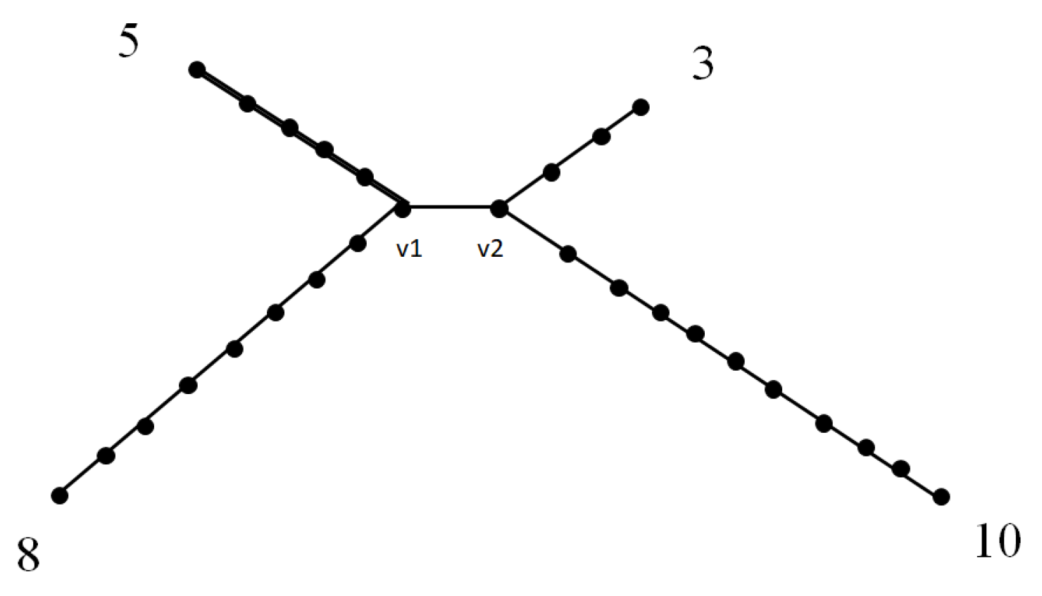
We consider a tree $T_{n,k}$ where k is an even integer. The lengths of the paths incident to the ‘center’ vertex v have lengths $k,2k,\dots ,nk$. The theorems in this subsection help identify trees with two or three vertices with the same $SD$ value.

In addition to $SD(i,i)$ = $SD(n,i+1)$, when $i=\left({\displaystyle \genfrac{}{}{0pt}{}{a}{2}}\right)$ or $\left({\displaystyle \genfrac{}{}{0pt}{}{a+1}{2}}\right)$, we observed an additional pair of vertices with the same $SD$ value for even values of k.

Theorem 3.

For all positive, even values of k and $i=⌊{\displaystyle \frac{n}{2}}⌋$, $SD(i,ki-{\displaystyle \frac{k}{2}})=SD(n,ki+{\displaystyle \frac{k}{2}})$.

Proof. 

We set $SD(i,ki-{\displaystyle \frac{k}{2}})=SD(n,ki+{\displaystyle \frac{k}{2}})$ and solve for i.

$$\begin{array}{cc}\hfill 0& =SD\left(n,ki+{\displaystyle \frac{k}{2}}\right)-SD\left(i,ki-{\displaystyle \frac{k}{2}}\right)\hfill \\ \hfill & ={\left(ki+{\displaystyle \frac{k}{2}}\right)}^2-{\left(ki-{\displaystyle \frac{k}{2}}\right)}^2-2k\left(n\left(ki+{\displaystyle \frac{k}{2}}\right)-i\left(ki-{\displaystyle \frac{k}{2}}\right)\right)+k\left(ki+{\displaystyle \frac{k}{2}}-ki+{\displaystyle \frac{k}{2}}\right)\left({\displaystyle \genfrac{}{}{0pt}{}{n+1}{2}}\right)\hfill \\ \hfill & =2k^{2}i-2k\left(kni+{\displaystyle \frac{kn}{2}}-k{i}^2+{\displaystyle \frac{ki}{2}}\right)+k^2{\displaystyle \frac{n^2+n}{2}}\hfill \\ \hfill & =2k^{2}i-2k^{2}ni-k^{2}n+2k^2{i}^2-k^{2}i+{\displaystyle \frac{k^2{n}^2}{2}}+{\displaystyle \frac{k^{2}n}{2}}\hfill \\ \hfill & =2k^2{i}^2+(k^2-2k^{2}n)i+{\displaystyle \frac{k^2{n}^2}{2}}-{\displaystyle \frac{k^{2}n}{2}}.\hfill \end{array}$$

Solving for i, we have the following:

$$\begin{array}{cc}\hfill i& ={\displaystyle \frac{(2k^{2}n-k^2)\pm \sqrt{{(k^2-2k^{2}n)}^2-4\left(2k^2\right)(\frac{k^2{n}^2}{2}-\frac{k^{2}n}{2})}}{4k^2}}\hfill \\ \hfill & ={\displaystyle \frac{(2k^{2}n-k^2)\pm \sqrt{k^4-4k^{4}n+4k^4{n}^2-4k^4{n}^2+4k^{4}n}}{4k^2}}\hfill \\ \hfill & ={\displaystyle \frac{(2k^{2}n-k^2)\pm k^2}{4k^2}}\hfill \\ \hfill & ={\displaystyle \frac{2n-1\pm 1}{4}}\hfill \\ \hfill i& ={\displaystyle \frac{n}{2}}\mathrm{or}{\displaystyle \frac{n-1}{2}}.\hfill \end{array}$$

□

The pattern $SD(i,ki-{\displaystyle \frac{k}{2}})=SD(n,ki+{\displaystyle \frac{k}{2}})$ has a solution for all n. Since ${\displaystyle \frac{k}{2}}$ must be an integer, we find that for even values of k, every tree has at least one set of two vertices with the same $SD$ value.

Theorem 4.

$T_{n,2}$ has a pair vertices with the same $SD$ value, and in the case where $n=a^2+1$, there are three pairs of vertices with the same $SD$ value.

Proof. 

First, Lemmas 1 and 3 tell us that for $k=2$, equal vertices must be exactly two rows apart. Based on Theorem 3, we have that every $T_{n,2}$ has exactly one pair of equal vertices of the form $(i,2i-1)$ and $(n,2i+1)$. Lemma 5 gives two additional pairs of equal vertices when $n=a^2+1$.

To rule out other cases of vertices having the same $SD$, we start by looking at $(i,2i)$ and $(n-1,2i+2)$. If $SD(i,2i)=SD(n-1,2i+2)$, we obtain the following:

$$\begin{array}{cc}\hfill 0=& (2i+2-2i)(n^2+n+4i+2)-4((n-1)(2i+2)-2i^2)\hfill \\ \hfill & 8i^2+(16-8n)i+(2n^2-6n+12).\hfill \end{array}$$

We find that the discriminant of this quadratic is negative, so they can never be equal. As a consequence, we also have $SD(n-1-k,2i+2+j)>SD(i,2i)$ for all $k,j\ge 0$. We then look at $(i+1,2i)$ and $(n,2i+2)$. We set $SD(i+1,2i)=SD(n,2i+2)$ and will show that there are no values of i and n that make this equation true.

$$\begin{array}{cc}\hfill 0& =2(n^2+n+4i+2)-4(n(2i+2)-2i(i+1))\hfill \\ \hfill & =2n^2+2n+8i+4-8ni-8n+8i^2+8i\hfill \\ \hfill & =8i^2+(16-8n)i+(2n^2-6n+4).\hfill \end{array}$$

Finding the discriminant of this quadratic, we obtain the following:

$$\begin{array}{cc}\hfill \mathsf{\Delta }& =64{(2-n)}^2-32(2n^2-6n+4)\hfill \\ \hfill & =4-4n+n^2-n^2+3n-2\hfill \\ \hfill & =2-n.\hfill \end{array}$$

This is negative for $n>2$, so we have $SD(n,2i+2)>SD(i+k,2i-j)$ for all $k,j\ge 0$.

We next consider $(i,2i-1)$ and $(n-1,2i+1)$. If $SD(i,2i-1)=SD(n-1,2i+1)$, we obtain the following:

$$\begin{array}{cc}\hfill 0& =2(n^2+n+4i)-4((n-1)(2i+1)-2i^2-i)\hfill \\ \hfill & =2n^2+2n+8i-4(2ni+n-2i-1-2i^2-i)\hfill \\ \hfill & =2n^2+2n+8i-8ni-4n+8i+4+8i^2+4i\hfill \\ \hfill & =2n^2-2n+20i-8ni+4+8i^2\hfill \\ \hfill & =8i^2+(20-8n)i+(2n^2-2n+4).\hfill \end{array}$$

Finding the discriminant of this quadratic, we obtain the following:

$$\begin{array}{cc}\hfill \mathsf{\Delta }& =16{(5-2n)}^2-32(2n^2-2n+4)\hfill \\ \hfill & =25-20n+4n^2-4n^2+4n-8\hfill \\ \hfill & =17-16n.\hfill \end{array}$$

This is negative for $n>1$, so we have $SD(n-1-k,2i+1+j)>SD(i,2i-1)$ for all $k,j\ge 0$. Finally, we look at $(i+1,2i-1)$ and $(n,2i+1)$.

$$\begin{array}{cc}\hfill 0& =2(n^2+n+4i)-4(n(2i+1)-(i+1)(2i-1))\hfill \\ \hfill & =2n^2+2n+8i-4(2ni+n-(2i^2-i+2i-1))\hfill \\ \hfill & =2n^2+2n+8i-8ni-4n+8i^2+4i-8i+4\hfill \\ \hfill & =8i^2+(4-8n)i+(2n^2-2n+4).\hfill \end{array}$$

Finding the discriminant of this quadratic, we obtain the following:

$$\begin{array}{cc}\hfill \mathsf{\Delta }& =16{(1-2n)}^2-32(2n^2-2n+4)\hfill \\ \hfill & =1-4n+4n^2-4n^2+4n-8\hfill \\ \hfill & =-7.\hfill \end{array}$$

Since the discriminant is negative, we have $SD(n,2i+1)>SD(i+1+k,2i-1-j)$ for all $k,j\ge 0$.

Combining the four previous results, the only possible solutions for even k have the form $SD(i,2i)=SD(n,2i+2)$, and $SD(i,2i-1)=SD(n,2i+1)$. □

2.2. Triple Values

In the previous section, we identified asymmetric trees that have pairs of vertices with the same $SD$ value. However, we found asymmetric trees that have a ‘triple’: three vertices with the same $SD$ value. For example, when $k=3$, $n=6$, $SD(2,5)=SD(6,8)=SD(5,7)$; when $k=6$, $n=6$, $SD(2,10)=SD(5,14)=SD(6,16)$; and when $k=8$, $n=4$, $SD(1,6)=SD(3,10)=SD(4,14)$. In this section, we will expand these to infinite families of graphs with three vertices that have the same $SD$ value.

In Table 1, we see that triples occur for different values of n and k. Many of the even cases are verified in the theorems in this section. Other patterns were not as easily categorized.

Table 1. Existence of triples for different n and k values.

n	k Values	Form of k
4	4, 8, 12, …	$4u$ and $12w$
6	3, 6, 9, …	$3u$ and $15w$
8	8, 16, 24, …	$8u$
10	5, 10, 15, …	$5u$
12	12, 24, 36, …	$12u$ and $84w$
14	7, 14, 21, …	$7u$
7	12, 24, 36, …	$12u$
9	20, 35, 40, 60, 70, …	$20u$ and $35w$
11	36, 72, 108, …	$36u$
13	28, 56, 84, …	$28u$
15	44, 60, 76, 88, …	$44u$, $76w$, and $76z$

We observe that when ${\displaystyle \frac{n}{2}}$ is even, a triple exists when k is a multiple of n. When ${\displaystyle \frac{n}{2}}$ is odd, k is a multiple of ${\displaystyle \frac{n}{2}}$. Some values of k also have a second set of triples.

Since the j values change depending on k, we divide the j values into segments and locations. Each segment is of length k, the first going from rows $1,2,\dots ,k$, the second from rows $k+1,k+2,\dots ,2k$, continuing until the last segment from $(n-1)k+1,(n-1)k+2,\dots ,nk$. The location in the segment is numbered by how far from the top of the segment the vertex is.

For example, for the tree $T_{3,5}$ with branches of lengths 5, 10, and 15, the vertex (2, 7) is in the second segment at location 2. This is illustrated in Figure 4.

Figure 4. Segments and locations for $T_{3,5}$.

We can then represent j using segments and locations.

$$j=(\mathrm{segment}-1)k+\mathrm{location}$$

We next explore trees where we scale k by a constant and see that the pairs of vertices with equal $SD$ values scale accordingly.

Lemma 6.

Let $c>1$. If $SD(i,j)=SD(l,m)$ for $T_{n,k}$, then $SD(i,cj)=SD(l,cm)$ for $T_{n,ck}$.

Proof. 

We see that for $T_{n,k}$, using the $SD$ formula,

$$\begin{array}{c}\hfill (j-m)\left(k\left({\displaystyle \genfrac{}{}{0pt}{}{n+1}{2}}\right)+j+m\right)-2k(ij-lm)=0\end{array}$$

Then, substituting $cj$ for j and $cm$ for m,

$$\begin{array}{cc}\hfill SD(i,cj)-SD(l,cm)& =(cj-cm)\left(ck\left({\displaystyle \genfrac{}{}{0pt}{}{n+1}{2}}\right)+cj+cm\right)-2ck(cij-clm)\hfill \\ \hfill & =c^2(SD(i,j)-SD(l,m))\hfill \\ \hfill & =c^2\left(0\right)\hfill \\ \hfill & =0\hfill \end{array}$$

□

Previously, we found two main patterns for triples for even n values. The first occurred when ${\displaystyle \frac{n}{2}}\equiv 0mod2$. Here, we note that there are three vertices with the same $SD$ value when k is a multiple of n.

Observing this pattern in Table 2, for each n value, the i values of the matching vertices remain the same. For example, for $n=4$, the i values are 1, 3, and 4. For $n=8$, the i values are 3, 7, and 8. We will show in Theorem 5 that the i values are ${\displaystyle \frac{n}{2}}-1,n-1,\mathrm{and}n$.

Table 2. Existence of triples where both n and k are multiples of 4.

n	k	Vertices
4	4	(1, 3), (3, 5), and (4, 7)
4	8	(1, 6), (3, 10), and (4, 14)
4	12	(1, 9), (3, 15), and (4, 21)
8	8	(3, 21), (7, 27), and (8, 29)
8	16	(3, 42), (7, 54), and (8, 58)
12	12	(5, 55), (11, 65), and (12, 67)
16	16	(7, 105), (15, 119), and (16, 121)

Finding the segments for the triple, we see that for $n=4$, the leftmost vertex appears in the first segment, while the other two vertices occur in the second segment. For $n=8$, the leftmost vertex appears in the third segment, and the others appear in the fourth. When ${\displaystyle \frac{n}{2}}$ is odd, a similar pattern appears.

Next, we checked the locations of the vertices. The vertex (1, 3) for $n=4,k=4$ is located in the first segment at location 3, the vertex (3, 5) is in segment 2 at location 1, and the vertex (4, 7) is in segment 2 at location 3. Note that in Table 3, for $n=4,k=8$, the locations are scalar multiples of the locations for $n=4,k=4$.

Table 3. Existence of triples for different n and k values with segments and locations.

n	Segments	n	k	Locations
4	1, 2, and 2	4	4	3, 1, and 3
6	2, 3, and 3	4	8	6, 2, and 6
8	3, 4, and 4	8	8	5, 3, and 5
10	4, 5, and 5	12	12	7, 5, and 7
12	5, 6, and 6	16	16	9, 7, and 9
14	6, 7, and 7
16	7, 8, and 8

To generalize this, the segments in which the triples appear when n is even are ${\displaystyle \frac{n}{2}}-1,{\displaystyle \frac{n}{2}},\mathrm{and}{\displaystyle \frac{n}{2}}$. Then, generalizing the locations for when ${\displaystyle \frac{n}{2}}$ is even, we have ${\displaystyle \frac{n}{2}}+1,{\displaystyle \frac{n}{2}}-1,$$\mathrm{and}{\displaystyle \frac{n}{2}}+1$.

Theorem 5.

When $k=n=2w$, the vertices $(w-1,2w^2-3w+1)$, $(2w-1,2w^2-w-1)$, and $(2w,2w^2-w+1)$ have equal $SD$ values.

Proof. 

Let $Z=SD(0,0)$.

Using Equation (1), we have the following:

$$\begin{array}{cc}\hfill SD(w-1,2w^2-3w+1)& =Z+{(2w^2-3w+1)}^2-2\left(2w\right)(w-1)(2w^2-3w+1)+\left(2w\right)(2w^2-3w+1)\left({\displaystyle \genfrac{}{}{0pt}{}{2w+1}{2}}\right)\hfill \\ \hfill & =Z+8w^5-12w^4+6w^3-w^2-2w+1.\hfill \\ \hfill SD(2w-1,2w^2-w-1)& =Z+{(2w^2-w-1)}^2-2\left(2w\right)(2w-1)(2w^2-w-1)+\left(2w\right)(2w^2-w-1)\left({\displaystyle \genfrac{}{}{0pt}{}{2w+1}{2}}\right)\hfill \\ \hfill & =Z+8w^5-12w^4+6w^3-w^2-2w+1.\hfill \\ \hfill SD(2w,2w^2-w+1)& =Z+{(2w^2-w+1)}^2-2\left(2w\right)\left(2w\right)(2w^2-w+1)+\left(2w\right)(2w^2-w+1)\left({\displaystyle \genfrac{}{}{0pt}{}{2w+1}{2}}\right)\hfill \\ \hfill & =Z+8w^5-12w^4+6w^3-w^2-2w+1.\hfill \end{array}$$

Since these three pairs have the same $SD$ value, there is a triple. □

The above proof works for $n=2w$ and $k=2w$. Lemma 6 shows that if two vertices have equal $SD$ values, then scaling k by a constant results in vertices with the same $SD$ values with the same i values and j values scaled by the same constant as k in the new tree.

When $n=2w$ and $k=2wc$, the vertices $(w-1,2w^{2}c-3wc+c)$, $(2w-1,2w^{2}c$$-wc-c)$, and $(2w,2w^{2}c-wc+c)$ have equal $SD$ values.

Next, consider when ${\displaystyle \frac{n}{2}}$ is odd. When ${\displaystyle \frac{n}{2}}\equiv 1mod2$, vertices with equal $SD$ values appear when k is a multiple of ${\displaystyle \frac{n}{2}}$. The i values of the triple are ${\displaystyle \frac{n}{2}}-1,n-1,\mathrm{and}n$. The j segments are ${\displaystyle \frac{n}{2}}-1,{\displaystyle \frac{n}{2}},\mathrm{and}{\displaystyle \frac{n}{2}}$. We show triples for various values of n and k in Table 4.

Table 4. Triples for different n and k values with segments and locations.

n	k	Vertices	n	k	Locations
6	3	(2, 5), (5, 7), and (6, 8)	6	3	2, 1, and 2
6	6	(2, 10), (5, 14), and (6, 16)	10	5	3, 2, and 3
10	5	(4, 18), (9, 22), and (10, 23)	14	7	4, 3, and 4
10	10	(4, 36), (9, 44), and (10, 46)	18	9	5, 4, and 5
14	7	(6, 39), (13, 45), and (14, 46)
18	9	(8, 68), (17, 76), and (18, 77)

Let $n=2(2b+1)$ and $k=2b+1$. Then, the i values can be represented as $2b,$ 4b+1,$\mathrm{and}4b+2$. The j segments can be written as $2b,2b+1,$$\mathrm{and}2b+1$. Finally, the locations can be represented as $b+1,b,\mathrm{and}b+1$.

Theorem 6.

When $n=2(2b+1)$ and $k=2b+1$, the three vertices $(2b,4b^2+b)$, $(4b+1,4b^2+3b)$, and $(4b+2,4b^2+3b+1)$ have equal SD values.

Proof. 

Let $Z=SD(0,0)$. Using Equation (1), we have the following:

$$\begin{array}{cc}\hfill SD(2b,4b^2+b)& =Z+{(4b^2+b)}^2-2(2b+1)\left(2b\right)(4b^2+b)+(2b+1)(4b^2+b)\left({\displaystyle \genfrac{}{}{0pt}{}{4b+3}{2}}\right)\hfill \\ \hfill & =64b^5+112b^4+76b^3+25b^2+3b.\hfill \\ \hfill SD(4b+1,4b^2+3b)& =Z+{(4b^2+3b)}^2-2(2b+1)(4b+1)(4b^2+3b)+(2b+1)(4b^2+3b)\left({\displaystyle \genfrac{}{}{0pt}{}{4b+3}{2}}\right)\hfill \\ \hfill & =64b^5+112b^4+76b^3+25b^2+3b.\hfill \\ \hfill SD(4b+2,4b^2+3b+1)& =Z+{(4b^2+3b+1)}^2-2(2b+1)(4b+2)(4b^2+3b+1)+(2b+1)(4b^2+3b+1)\left({\displaystyle \genfrac{}{}{0pt}{}{4b+3}{2}}\right)\hfill \\ \hfill & =64b^5+112b^4+76b^3+25b^2+3b.\hfill \end{array}$$

Since the $SD$ values are the same for all three vertices, they form a triple. □

Based on Lemma 6, when $n=2(2b+1)$ and $k=(2b+1)c$, the vertices $(2b,4b^{2}c+bc)$, $(4b+1,4b^{2}c+3bc)$, and $(4b+2,4b^{2}c+3bc+c)$ have equal $SD$ values.

When ${\displaystyle \frac{n}{2}}\equiv 0mod2$, there is a second pattern. We show these in Table 5.

Table 5. More patterns for triples.

n	k	Vertices	Segments	Locations
4	12	(2, 5), (4, 11), and (3, 7)	1, 1, 1	5, 11, 7
12	28	(6, 117), (10, 131), and ( 11, 135)	5, 5, 5	5, 19, 23
16	36	(8, 221), (13, 239), and (15, 247)	7, 7, 7	5, 23, 31
20	44	(10, 357), (16, 379), and (19, 291)	9, 9, 9	5, 27, 39
24	52	(12, 525), (19, 551), and (23, 567)	11, 11, 11	5, 31, 47

Let $n=4c$. There is a second pattern of triples when k is a multiple of $8c+4$. The i values are $2c,3c+1,\mathrm{and}4c-1$. The j segments are $2c-1$, and the locations within the segment are $5,4c+7,\mathrm{and}8c-1$.

Theorem 7.

When $n=4c$ and $k=8c+4$, $c\ne 2$, the vertices $(2c,16c^2-8c-3)$, $(3c+1,16c^2-4c-1)$, and $(4c-1,16c^2-9)$ have equal $SD$ values.

Proof. 

Let $Z=SD(0,0)$. Using the $SD$ formula for k-multiple trees, we obtain the following:

$$\begin{array}{cc}\hfill SD(2c,16c^2-8c-3)& =Z+{(16c^2-8c-3)}^2-2(8c+4)\left(2c\right)(16c^2-8c-3)+(8c+4)(16c^2-8c-3)\left({\displaystyle \genfrac{}{}{0pt}{}{4c+1}{2}}\right)\hfill \\ \hfill & =Z+1024c^5-704c^3-16c^2+72c+9.\hfill \\ \hfill SD(3c+1,16c^2-4c-1)& =Z+{(16c^2-4c-1)}^2-2(8c+4)(3c+1)(16c^2-4c-1)+(8c+4)(16c^2-4c-1)\left({\displaystyle \genfrac{}{}{0pt}{}{4c+1}{2}}\right)\hfill \\ \hfill & =Z+1024c^5-704c^3-16c^2+72c+9.\hfill \\ \hfill SD(4c-1,16c^2-9)& =Z+{(16c^2-9)}^2-2(8c+4)(4c-1)(16c^2-9)+(8c+4)(16c^2-9)\left({\displaystyle \genfrac{}{}{0pt}{}{4c+1}{2}}\right)\hfill \\ \hfill & =Z+1024c^5-704c^3-16c^2+72c+9.\hfill \end{array}$$

Since these vertices have the same $SD$ value, they form a triple.

Now, consider when $c=2$. Then, $n=8,k=20$, and the three matching vertices are (4, 44), (7, 55), and (7, 55). Since the second and third vertices are the same, there is no triple for this pattern for $n=8$. □

Based on Lemma 6, when $n=4c$ and $k=(8c+4)g$, the vertices $(2c,16c^{2}g-8cg-3g)$, $(3c+1,16c^{2}g-4cg-g)$, and $(4c-1,16c^{2}g-9g)$ form a triple.

3. Trees with a Pair of Vertices with the Same $\mathit{SD}$ Value

In this section, we consider trees with a path connecting two vertices $v_1$ and $v_2$ with pendant paths incident to $v_1$ and $v_2$. We investigate sufficient conditions for $SD\left(v_1\right)=SD\left(v_2\right)$ with a surprising connection to combinatorial identities involving Pascal’s triangle.

Lemma 7.

Let G be a tree with vertices $v_1$ and $v_2$ with a path with t vertices connecting them and with pendant paths incident to $v_1$ and $v_2$. If there is an equal number of vertices on the two sides of the path with end-vertices $v_1$ and $v_2$, then $SD\left(v_1\right)=SD\left(v_2\right)$.

Proof. 

We can proceed by induction on the number of vertices in the tree. For the base case, there are zero vertices on each side of the path, and $SD\left(v_1\right)=SD\left(v_2\right)$ by symmetry. Next, assume the property holds for graphs with k vertices on each side of the path connecting $v_1$ and $v_2$. Then, consider a graph G where there are $k+1$ vertices on each side of the path connecting $v_1$ and $v_2$. Then, we remove vertex $v_a$ from the side with $v_1$ distance a from $v_1$ and remove a vertex $v_b$ from the side with $v_2$ distance b from $v_2$. Then, $SD\left(v_1\right)$ and $SD\left(v_2\right)$ will each decrease by $a+b+t$. □

Example 1.

Consider the asymmetric tree shown in Figure 5.

Figure 5. A graph where $SD\left(v_1\right)=SD\left(v_2\right)$.

Based on Lemma 7, $SD\left(v_1\right)=SD\left(v_2\right)$. Then, their corresponding algebraic expressions are equal. $SD\left(v_1\right)+1=SD\left(v_2\right)+1$ implies $\left({\displaystyle \genfrac{}{}{0pt}{}{6}{2}}\right)$$+\left({\displaystyle \genfrac{}{}{0pt}{}{9}{2}}\right)$$+\left({\displaystyle \genfrac{}{}{0pt}{}{5}{2}}\right)$$+\left({\displaystyle \genfrac{}{}{0pt}{}{12}{2}}\right)=\left({\displaystyle \genfrac{}{}{0pt}{}{7}{2}}\right)$$+\left({\displaystyle \genfrac{}{}{0pt}{}{10}{2}}\right)$$+\left({\displaystyle \genfrac{}{}{0pt}{}{4}{2}}\right)$$+\left({\displaystyle \genfrac{}{}{0pt}{}{11}{2}}\right).$

We illustrate a connection to Pascal’s triangle in Figure 5. We present the following result for trees that have the same number of vertices on the two sides of the edge $v_1$$v_2$.

Theorem 8.

Suppose $a_i$ and $b_j$ are integers greater than or equal to 2 with $1\le i\le n$ and $1\le j\le m$, and let ℓ be an integer such that ℓ$\ge 2$. If

$$\sum _{i=1}^n{a}_i=\sum _{j=1}^m{b}_j,$$

then

$$\sum _{i=1}^n\left({\displaystyle \genfrac{}{}{0pt}{}{a_i}{2}}\right)+\sum _{j=1}^m\left({\displaystyle \genfrac{}{}{0pt}{}{b_j+\ell }{2}}\right)-m\left({\displaystyle \genfrac{}{}{0pt}{}{\ell +1}{2}}\right)=\sum _{i=1}^n\left({\displaystyle \genfrac{}{}{0pt}{}{a_i+\ell }{2}}\right)+\sum _{j=1}^m\left({\displaystyle \genfrac{}{}{0pt}{}{b_j}{2}}\right)-n\left({\displaystyle \genfrac{}{}{0pt}{}{\ell +1}{2}}\right).$$

Proof. 

Suppose we have a path from $v_1$ to $v_2$ of length l. Then, suppose we have n branches connected to $v_1$, each one being a pendant path of length $a_1-1,a_2-1,\cdots ,a_n-1$, and we have m branches connected to $v_2$, each one being a pendant path of length $b_1-1,b_2-1,\cdots ,b_m-1$. If the number of vertices on each side are the same, then ${\sum }_{i=1}^n{a}_i={\sum }_{j=1}^n{b}_j$, and we the sums of the distances are equal. For a path of length $a_i-1$, $S{D}_{a_i-1}\left(v_1\right)=\left({\displaystyle \genfrac{}{}{0pt}{}{a_i}{2}}\right)$, and for a path of length $b_j-1$, $S{D}_{b_j-1}\left(v_1\right)=\left({\displaystyle \genfrac{}{}{0pt}{}{b_j+l}{2}}\right)$. However, we are counting the path of length ℓ, $m-1$ extra times. Therefore, we have

$$SD\left(v_1\right)=\sum _{i=1}^n\left({\displaystyle \genfrac{}{}{0pt}{}{a_i}{2}}\right)+\sum _{j=1}^n\left({\displaystyle \genfrac{}{}{0pt}{}{b_j+\ell }{2}}\right)-(m-1)\left({\displaystyle \genfrac{}{}{0pt}{}{\ell +1}{2}}\right),$$

and similarly,

$$SD\left(v_2\right)=\sum _{i=1}^n\left({\displaystyle \genfrac{}{}{0pt}{}{a_i+\ell }{2}}\right)+\sum _{j=1}^n\left({\displaystyle \genfrac{}{}{0pt}{}{b_j+1}{2}}\right)-(n-1)\left({\displaystyle \genfrac{}{}{0pt}{}{\ell +1}{2}}\right).$$

Since $SD\left(v_1\right)=SD\left(v_2\right)$, the proof is complete. □

Corollary 1.

Let $a,b,c,d$ be integers greater than or equal to 2, with $a+b=c+d$. Then, $\left({\displaystyle \genfrac{}{}{0pt}{}{a}{2}}\right)$$+\left({\displaystyle \genfrac{}{}{0pt}{}{b}{2}}\right)$$+\left({\displaystyle \genfrac{}{}{0pt}{}{c+1}{2}}\right)$$+\left({\displaystyle \genfrac{}{}{0pt}{}{d+1}{2}}\right)=\left({\displaystyle \genfrac{}{}{0pt}{}{a+1}{2}}\right)$$+\left({\displaystyle \genfrac{}{}{0pt}{}{b+1}{2}}\right)$$+\left({\displaystyle \genfrac{}{}{0pt}{}{c}{2}}\right)$$+\left({\displaystyle \genfrac{}{}{0pt}{}{d}{2}}\right)$.

We also note that as a consequence of Theorem 8, the squares and circles can be shifted to the left by 1 to illustrate $4+7+10+11=5+6+9+12$ as shown in Figure 6.

Figure 6. A pattern arising from the tree in Figure 5.

4. Conclusions

In this paper, we investigated asymmetric trees including a ‘center’ vertex v with pendant paths of lengths $k,2k,\dots ,nk$. We completely characterized when there are pairs of vertices with the same $SD$ value for $k=1$ and $k=2$. $SD$ values for asymmetric trees with a vertex v of degree n and pendant paths of lengths $1,3,5,\dots ,2n-1$ were investigated as $SD$ values for some asymmetric graphs [8]. It would be an interesting problem to extend the results to the case where $k\ge 3$. A more general problem would be to extend these results for all asymmetric trees. We identified some asymmetric trees where three vertices have the same $SD$ value, but we did not encounter asymmetric trees with four or more vertices with the same $SD$ value. As a possible future study, we pose the following question.

Question. In an asymmetric tree with n vertices, what is the maximum number of vertices with the same $SD$ value?

References

- Sporns, O. Networks of the Brain; MIT Press: Cambridge, MA, USA, 2010. [Google Scholar]
- Bavelas, A. Communication Patterns in Task-Oriented Groups. J. Acoust. Soc. Am. 1950, 22, 725–730. [Google Scholar] [CrossRef]
- Neudorf, J.; Ekstrand, C.; Kress, S.; Borowsky, R. Brain Structural Connectivity Predicts Brain Functional Complexity: Diffusion Tensor Imaging Derived Centrality Accounts for Variance in Fractal Properties of Functional Magnetic Resonance Imaging Signal. Neuroscience 2020, 438, 1–8. [Google Scholar] [CrossRef] [PubMed]
- Eballe, R.; Cabahug, I. Closeness Centrality of Some Graph Families. Closeness Cent. Some Graph Fam. 2021, 16, 1000–1009. [Google Scholar] [CrossRef]
- Floyd, R.W. Algorithm 97: Shortest path. Commun. ACM 1962, 5, 345. [Google Scholar] [CrossRef]
- Warshall, S. A theorem on boolean matrices. Commun. ACM 1962, 9, 11–12. [Google Scholar] [CrossRef]
- Erdős, P.; Rényi, A. Asymmetric graphs. Acta Math. Acad. Sci. Hung. 1963, 14, 295–315. [Google Scholar] [CrossRef]
- Ramanathan, N.; Ramirez, E.; Suzuki-Burke, D.; Narayan, D.A. Closeness Centrality in Asymmetric Graphs; AMS: Providence, RI, USA, 2024. [Google Scholar]
Disclaimer/Publisher’s Note: The statements, opinions and data contained in all publications are solely those of the individual author(s) and contributor(s) and not of MDPI and/or the editor(s). MDPI and/or the editor(s) disclaim responsibility for any injury to people or property resulting from any ideas, methods, instructions or products referred to in the content. |
© 2024 by the authors. Licensee MDPI, Basel, Switzerland. This article is an open access article distributed under the terms and conditions of the Creative Commons Attribution (CC BY) license (https://creativecommons.org/licenses/by/4.0/).