
Hierarchical Learning-Enhanced Chaotic Crayfish Optimization Algorithm: Improving Extreme Learning Machine Diagnostics in Breast Cancer

Abstract
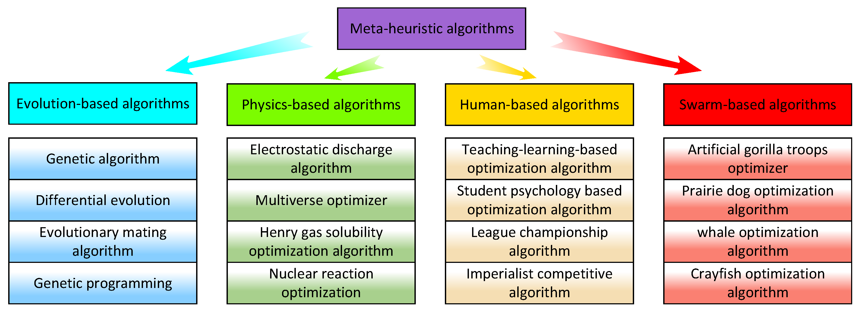
1. Introduction
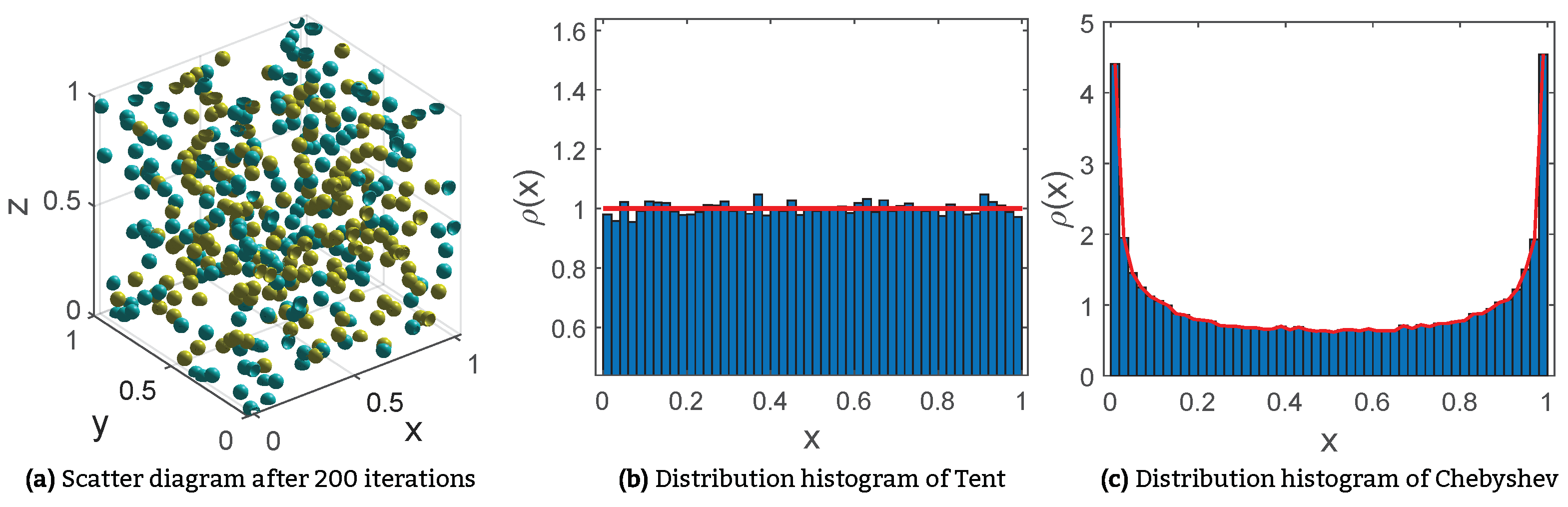
- Tent and Chebyshev maps are integrated into the HLCCOA for initializing the population, laying the foundation for subsequent global exploration by obtaining a high-quality initial population.
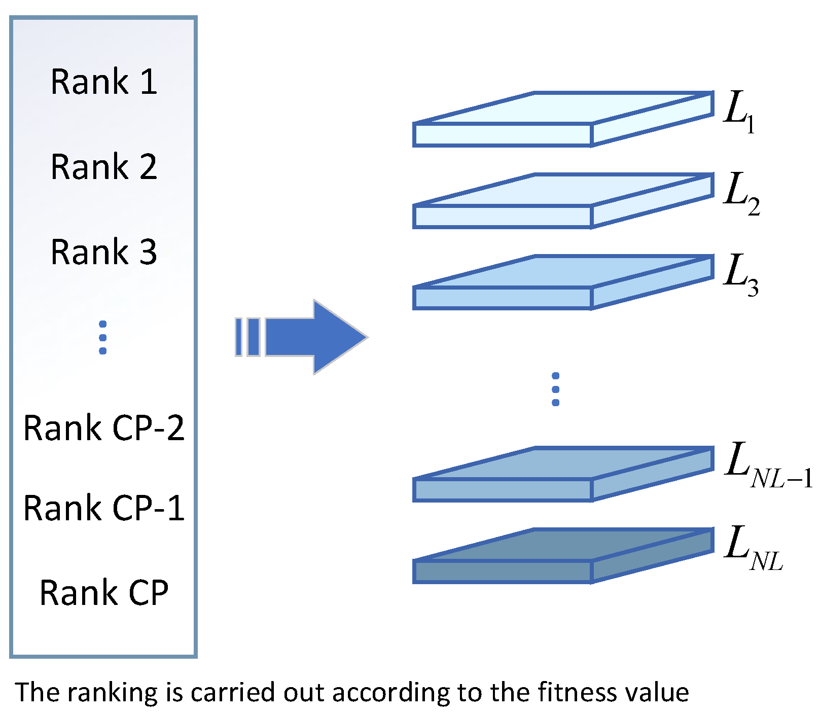
- A hierarchical learning mechanism is incorporated into the HLCCOA, which accelerates the convergence rate and improves the precision of optimization by strengthening the learning from exemplary individuals in each layer of the population.
- Comprehensive numerical experiments are designed. The HLCCOA is compared and analyzed against nine popular existing meta-heuristic optimization algorithms using the CEC2019 and CEC2022 suites, yielding favorable experimental results.
- An HLCCOA-ELM model for breast cancer diagnosis improves training by optimizing parameters to overcome local optima and raises accuracy, demonstrating the HLCCOA-ELM’s strong generalization performance.
2. Crayfish Optimization Algorithm
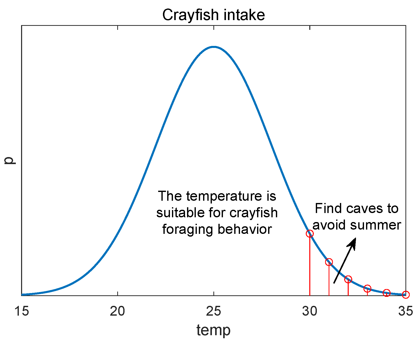
2.1. Summer Resort Pattern of Crayfish
2.2. Competition Pattern of Crayfish
2.3. Foraging Pattern of Crayfish
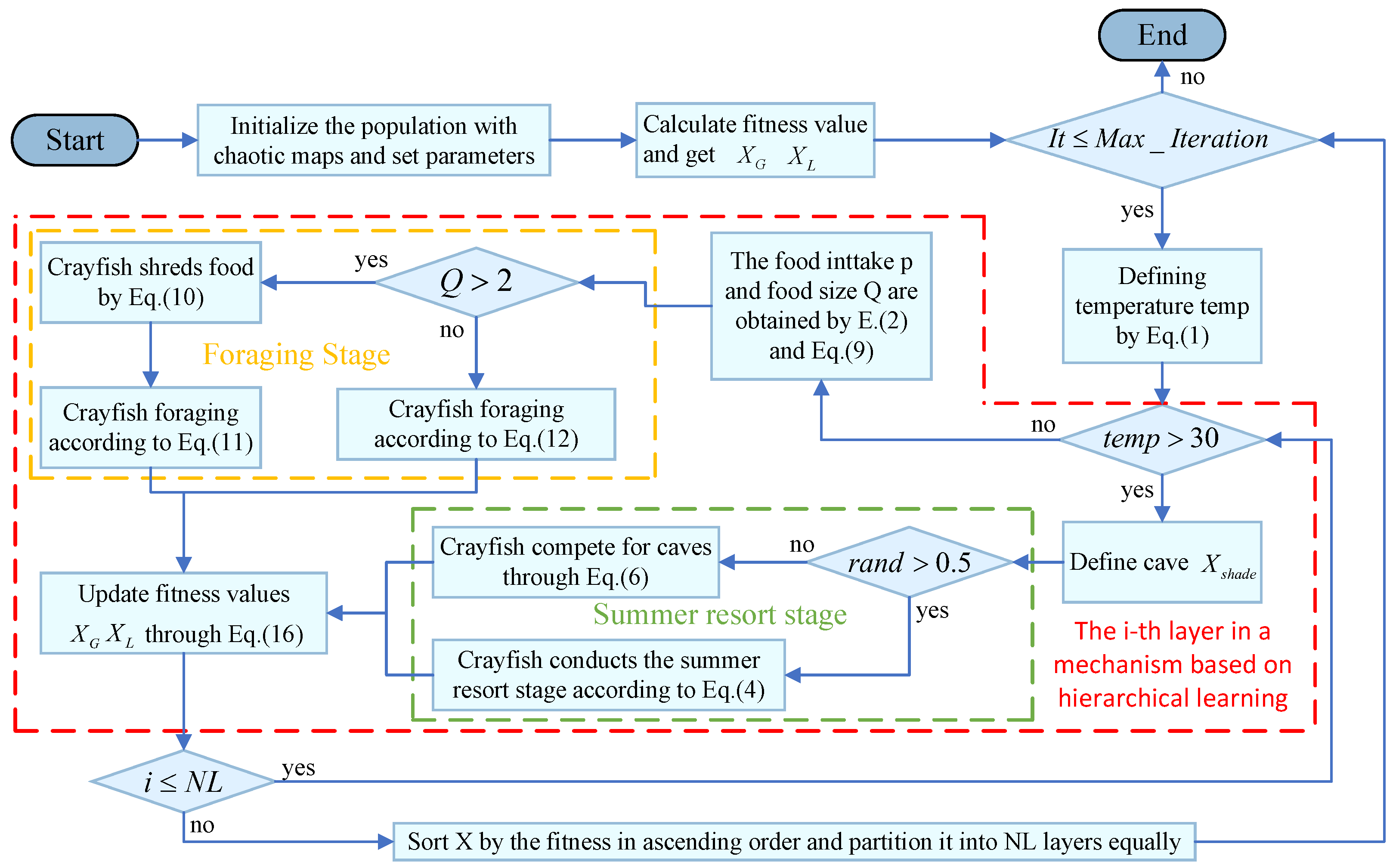
3. Hierarchical Learning-Based Chaotic Crayfish Optimization Algorithm
3.1. Chaotic Map
3.2. Hierarchical Learning Mechanism
| Algorithm 1 Pseudo-Code of the HLCCOA Algorithm |
|
4. Experimental Results and Discussion of the HLCCOA
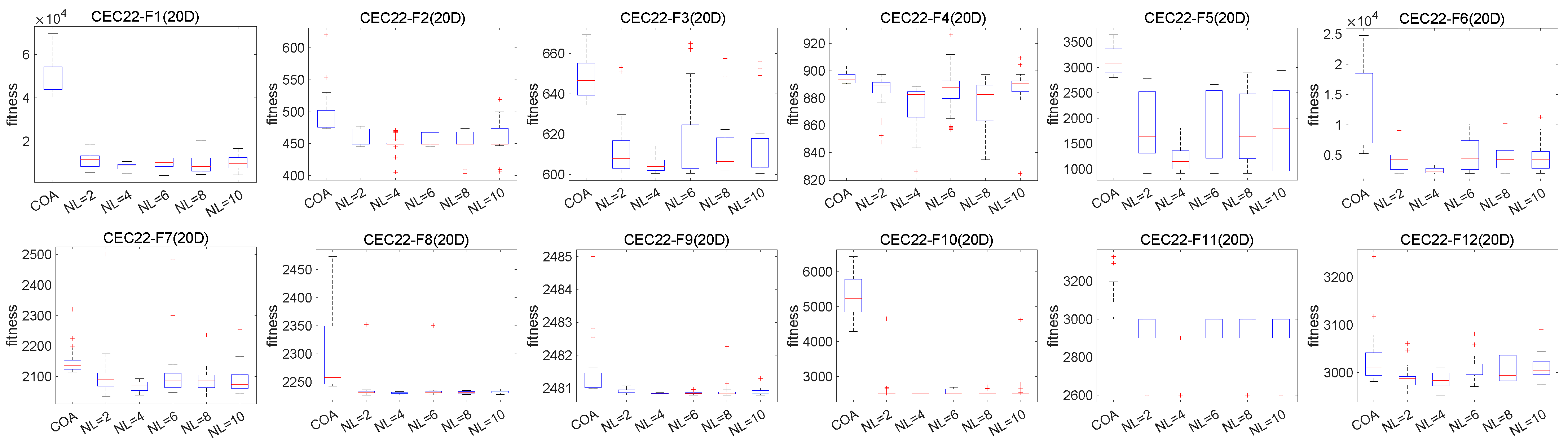
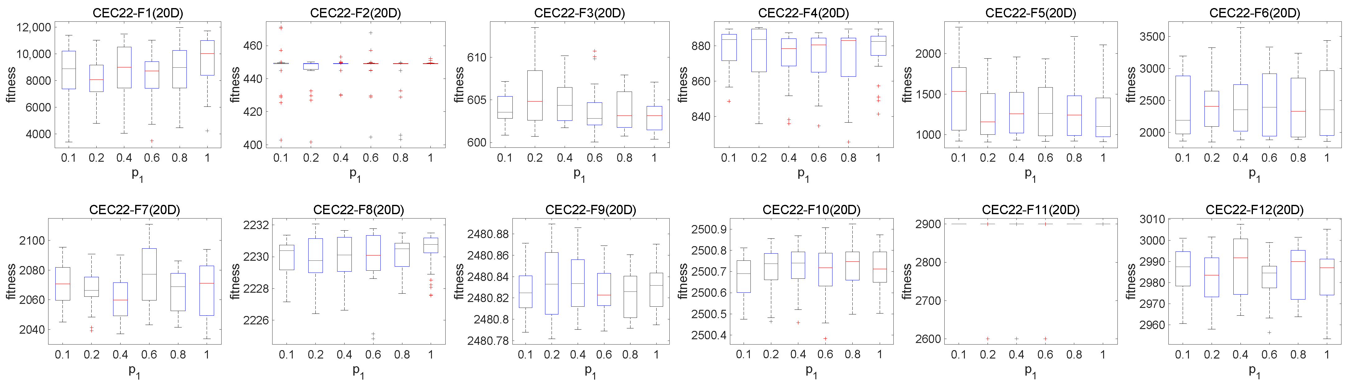
4.1. Parameter Analysis of the HLCCOA
4.2. Wilcoxon Signed-Rank Sum Test Results and Analysis
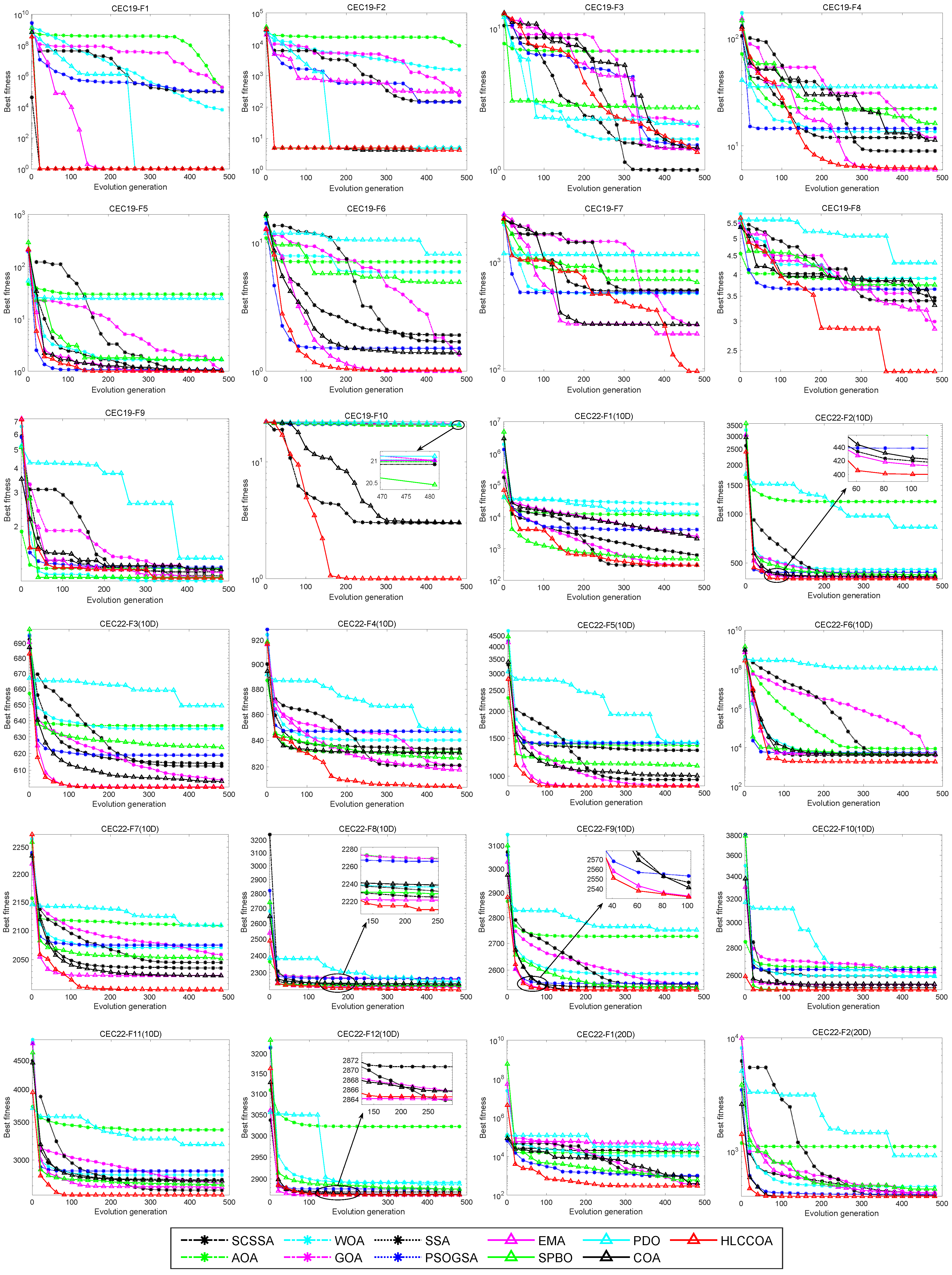
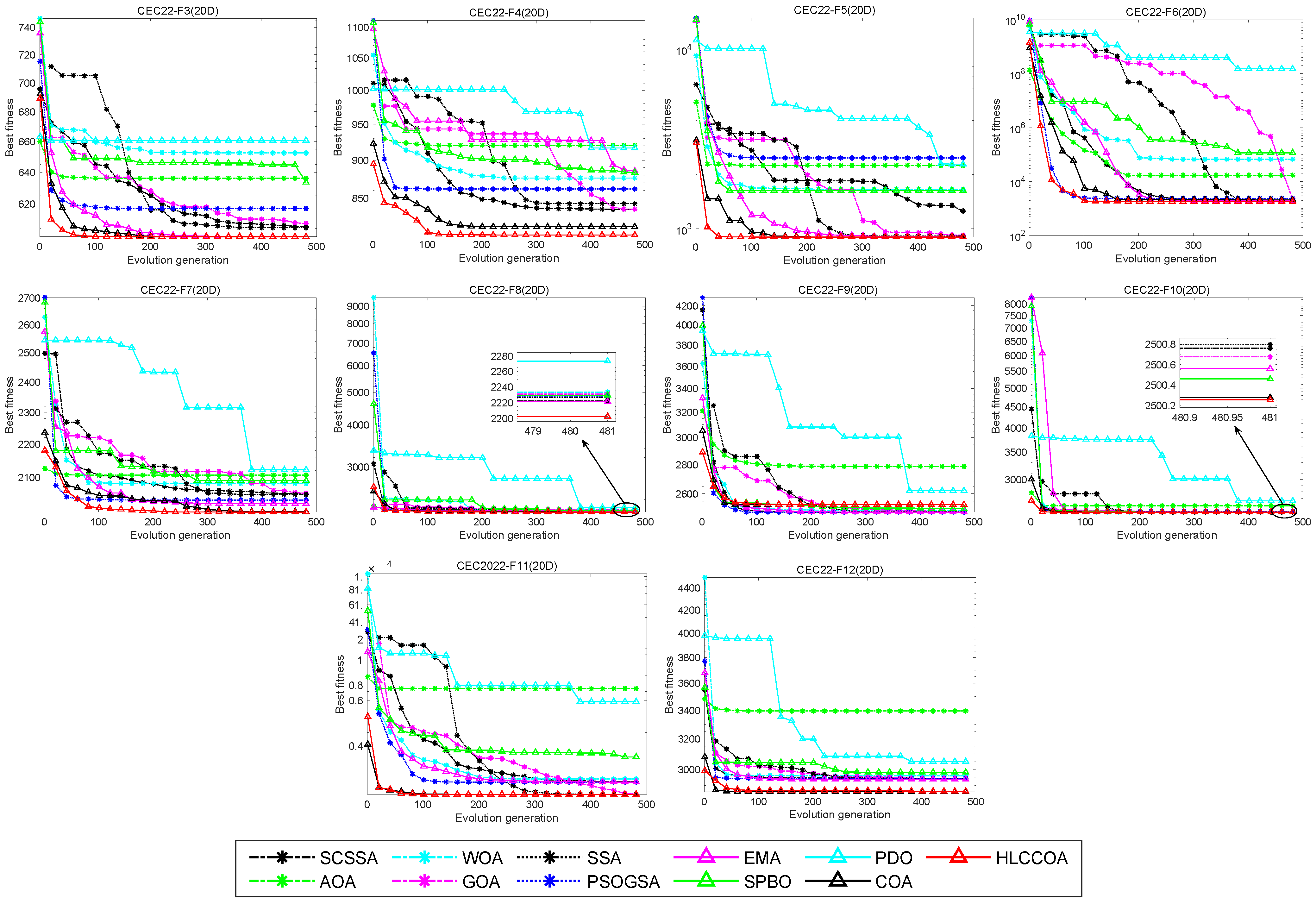
4.3. Convergence Curve Analysis
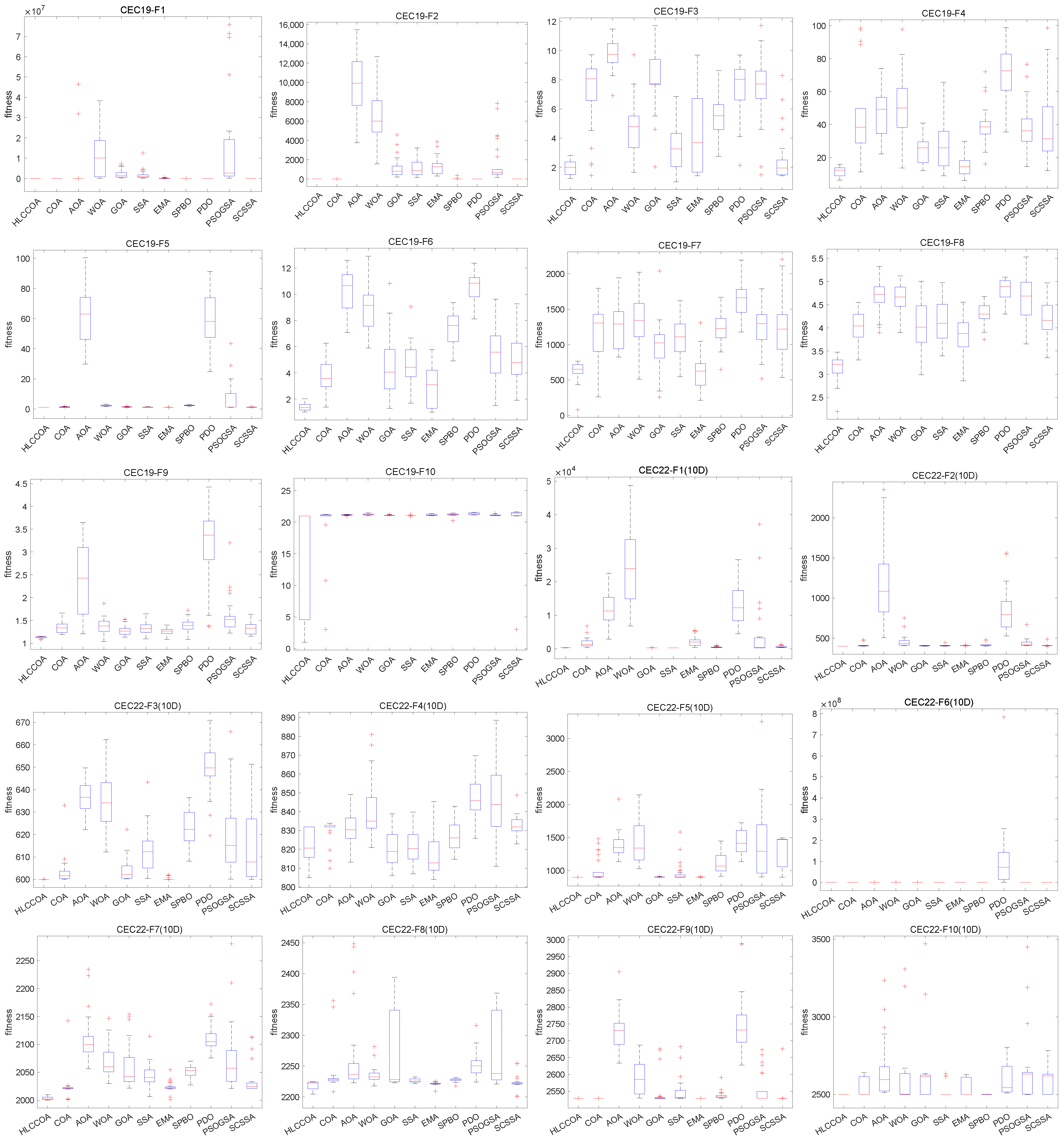
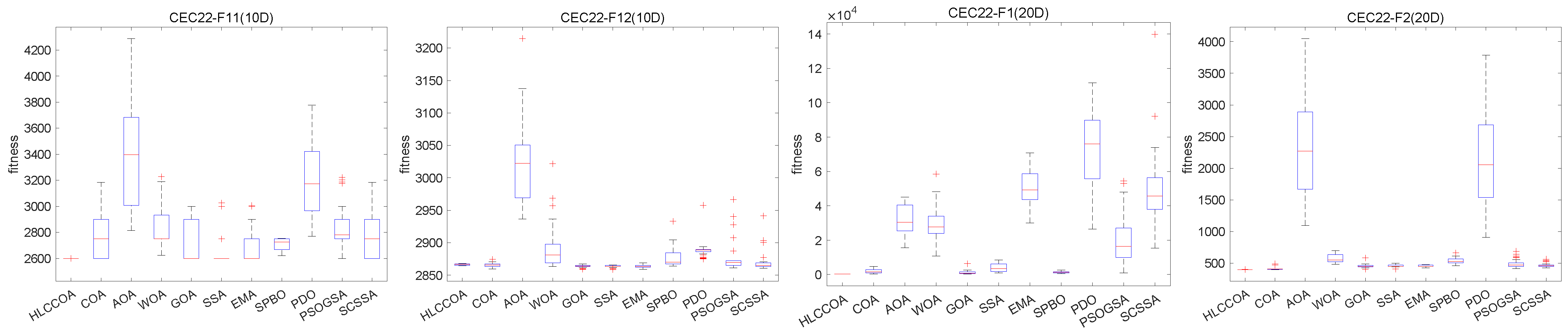
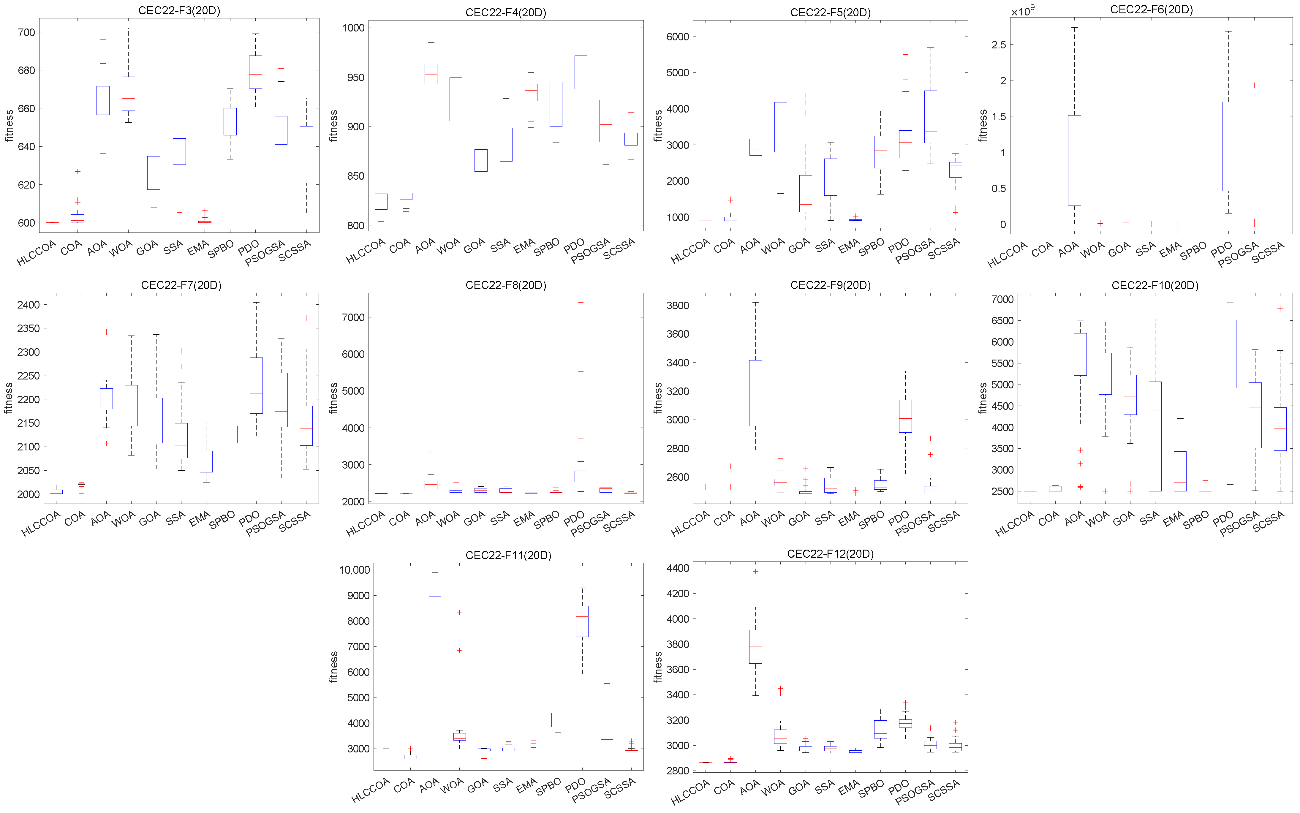
4.4. Analysis of Box Plot Results
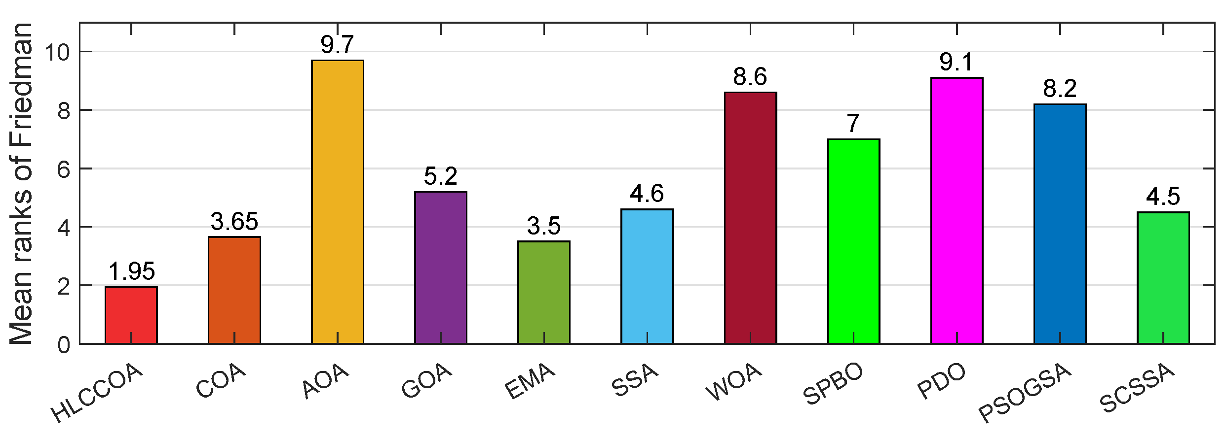
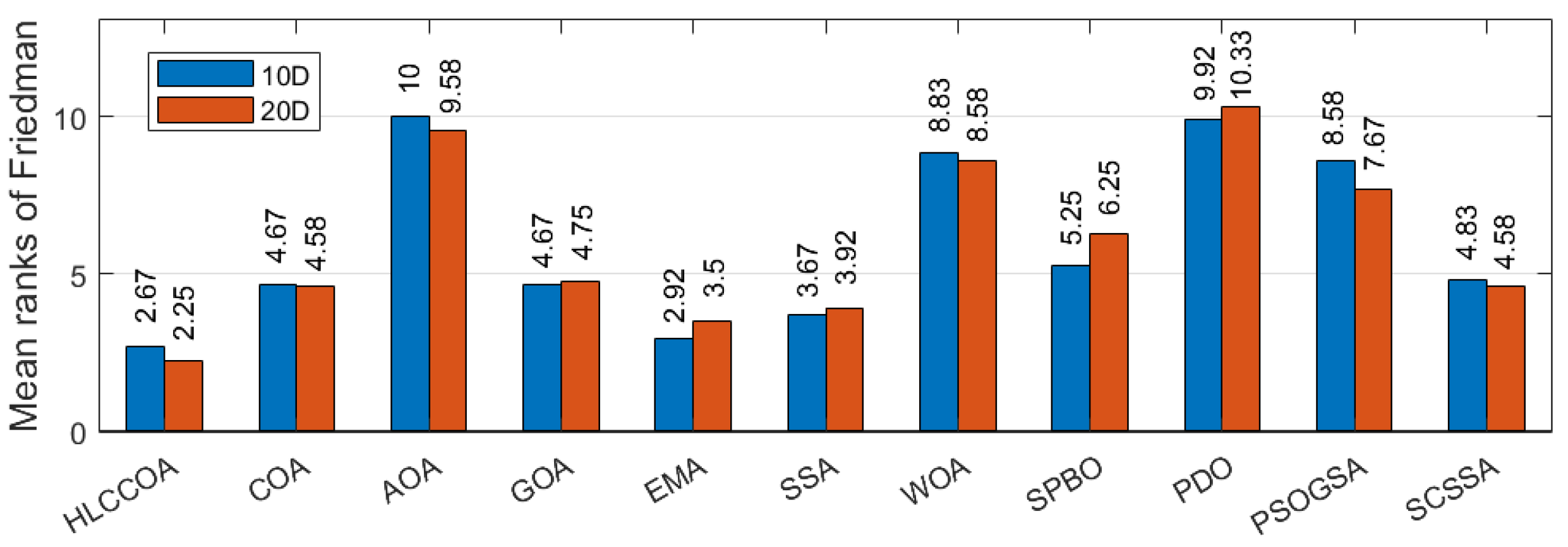
4.5. Friedman Test for the HLCCOA
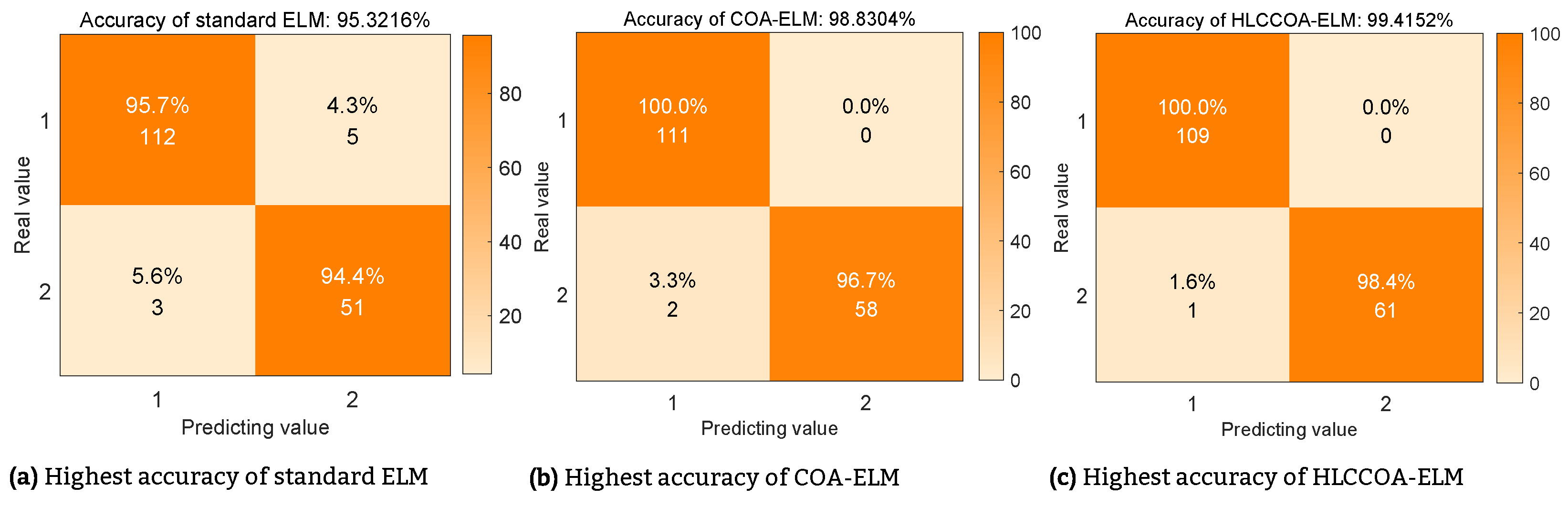
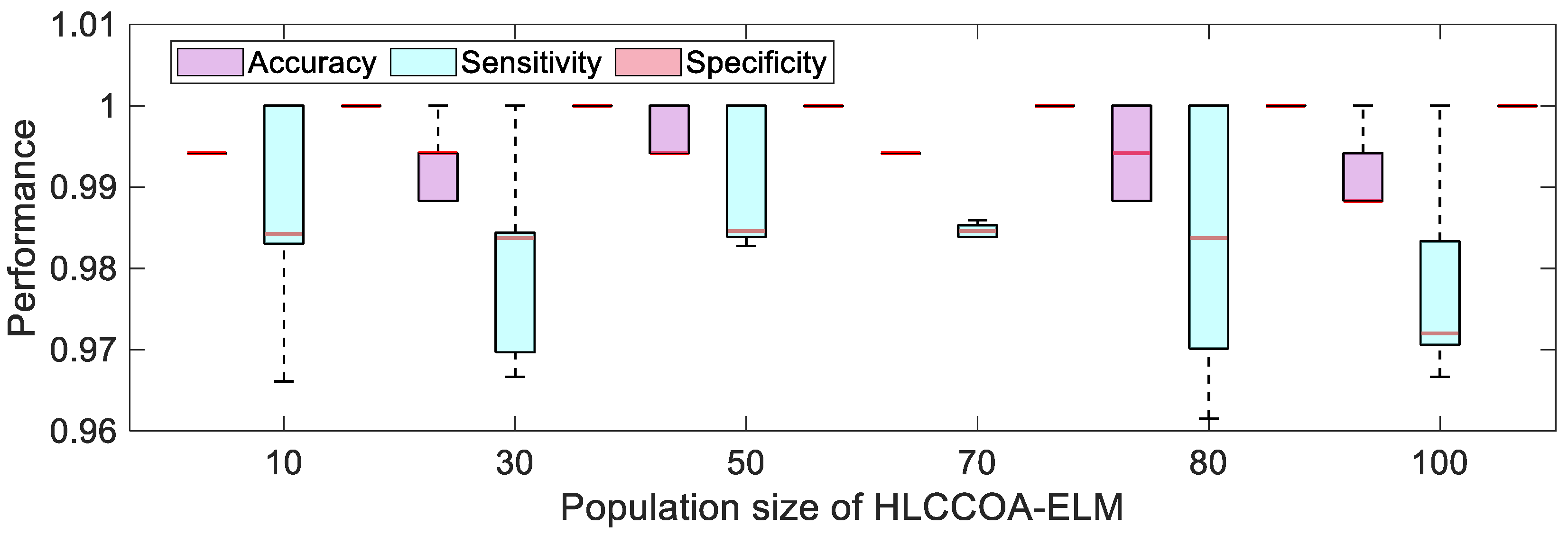
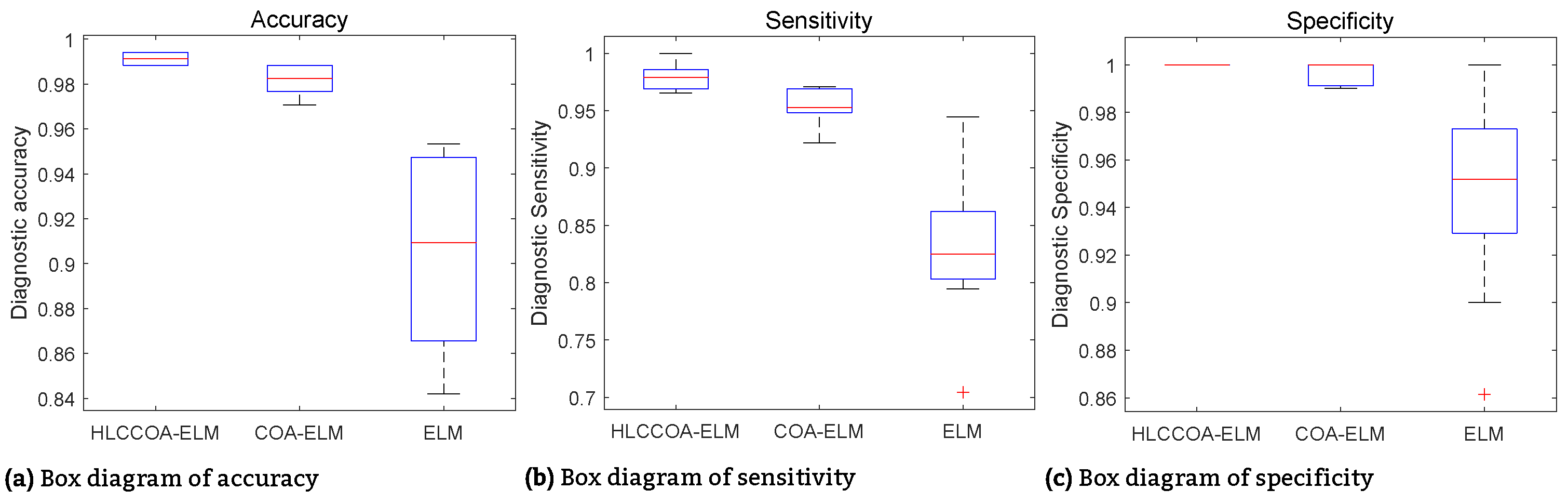
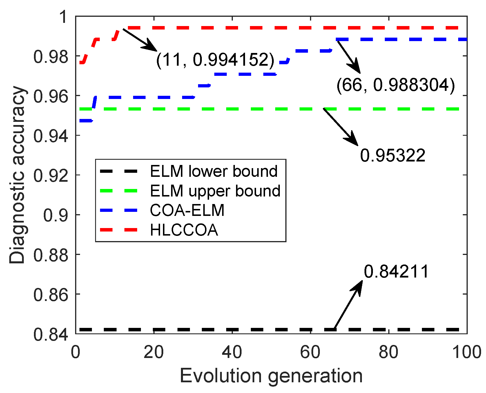
5. Breast Cancer Detection Based on the HLCCOA-ELM
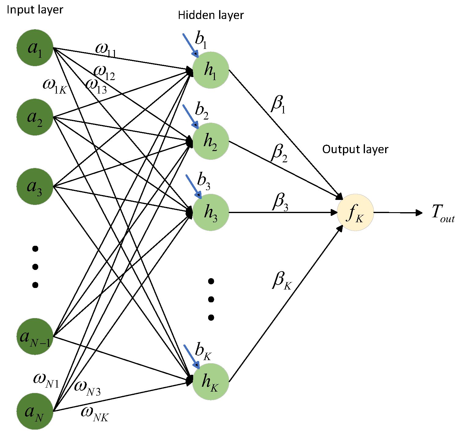
- Assume that the input of the ELM consists of N distinct samples , with a hidden layer composed of K neurons. Further, is the n-dimensional input vector for the i-th sample, and is the l-dimensional output vector for the i-th sample. Random values are assigned to the connection weights (, ) and to the biases () between the input and hidden layers. Subsequently, the hidden layer output matrix H is generated. The expression for H is as follows:
- The output function of the ELM can be expressed as follows:where represents the weight vector connecting the j-th hidden neuron to the output neurons, and denotes the collective set of weight vectors between the hidden layer and the output layer. To achieve the minimum training error for the network, it is necessary to find the least squares solution for the linear system , where T is the real output of the ELM. This training process can be represented through Equations (22) and (23):where represents the Moore–Penrose generalized inverse matrix of H. The final output of the network can be obtained using Equation (24):
6. Conclusions
Author Contributions
Funding
Data Availability Statement
Acknowledgments
Conflicts of Interest
References
- El-kenawy, E.-S.M.; Khodadadi, N.; Mirjalili, S.; Abdelhamid, A.A.; Eid, M.M.; Ibrahim, A. Greylag Goose Optimization: Nature-inspired optimization algorithm. Expert Syst. Appl. 2024, 238, 122–147. [Google Scholar] [CrossRef]
- Halim, A.H.; Ismail, I.; Das, S. Performance assessment of the metaheuristic optimization algorithms: An exhaustive review. Artif. Intell. Rev. 2021, 54, 2323–2409. [Google Scholar] [CrossRef]
- Sang, Y.; Tan, J.; Liu, W. Research on Many-Objective Flexible Job Shop A Modified Sand Cat Swarm Optimization Algorithm Based on Multi-Strategy Fusion and Its Application in Engineering Problems. Mathematics 2024, 12, 2153. [Google Scholar] [CrossRef]
- Zhu, F.; Li, G.; Tang, H.; Li, Y.; Lv, X.; Wang, X. Dung beetle optimization algorithm based on quantum computing and multi-strategy fusion for solving engineering problems. Expert Syst. Appl. 2024, 236, 121219. [Google Scholar] [CrossRef]
- Ozkaya, B.; Duman, S.; Kahraman, H.T.; Guvenc, U. Optimal solution of the combined heat and power economic dispatch problem by adaptive fitness-distance balance based artificial rabbits optimization algorithm. Expert Syst. Appl. 2024, 238, 122272. [Google Scholar] [CrossRef]
- Awwal, A.M.; Yahaya, M.M.; Pakkaranang, N.; Pholasa, N. A New Variant of the Conjugate Descent Method for Solving Unconstrained Optimization Problems and Applications. Mathematics 2024, 12, 2430. [Google Scholar] [CrossRef]
- Abualigah, L.; Elaziz, M.A.; Khasawneh, A.M.; Alshinwan, M.; Ibrahim, R.A.; Al-Qaness, M.A.A.; Mirjalili, S.; Sumari, P.; Gandomi, A.H. Meta-heuristic optimization algorithms for solving real-world mechanical engineering design problems: A comprehensive survey, applications, comparative analysis, and results. Neural Comput. Appl. 2022, 34, 4081–4110. [Google Scholar] [CrossRef]
- Miandoab, A.R.; Bagherzadeh, S.A.; Isfahani, A.H.M. Numerical study of the effects of twisted-tape inserts on heat transfer parameters and pressure drop across a tube carrying Graphene Oxide nanofluid: An optimization by implementation of Artificial Neural Network and Genetic Algorithm. Eng. Anal. Bound. Elem. 2022, 140, 1–11. [Google Scholar] [CrossRef]
- Pavlov-Kagadejev, M.; Jovanovic, L.; Bacanin, N.; Deveci, M.; Zivkovic, M.; Tuba, M.; Strumberger, I.; Pedrycz, W. Optimizing long-short-term memory models via metaheuristics for decomposition aided wind energy generation forecasting. Artif. Intell. Rev. 2024, 57, 45. [Google Scholar] [CrossRef]
- Huang, Q.; Ding, H.; Razmjooy, N. Oral cancer detection using convolutional neural network optimized by combined seagull optimization algorithm. Biomed. Signal Process. Control 2024, 87, 105546. [Google Scholar] [CrossRef]
- Zamani, H.; Nadimi-Shahraki, M.H. An evolutionary crow search algorithm equipped with interactive memory mechanism to optimize artificial neural network for disease diagnosis. Biomed. Signal Process. Control 2024, 90, 105879. [Google Scholar] [CrossRef]
- Deng, L.; Liu, S. Deficiencies of the whale optimization algorithm and its validation method. Expert Syst. Appl. 2024, 237, 121544. [Google Scholar] [CrossRef]
- MunishKhanna; Singh, L.K.; Garg, H. A novel approach for human diseases prediction using nature inspired computing & machine learning approach. Multimed. Tools Appl. 2024, 83, 17773–17809. [Google Scholar] [CrossRef]
- Cavallaro, C.; Cutello, V.; Pavone, M.; Zito, F. Machine Learning and Genetic Algorithms: A case study on image reconstruction. Knowl.-Based Syst. 2024, 284, 111194. [Google Scholar] [CrossRef]
- Formica, G.; Milicchio, F. Kinship-based differential evolution algorithm for unconstrained numerical optimization. Nonlinear Dyn. 2020, 99, 1341–1361. [Google Scholar] [CrossRef]
- Qiao, K.; Liang, J.; Qu, B.; Yu, K.; Yue, C.; Song, H. Differential Evolution with Level-Based Learning Mechanism. Complex Syst. Model. Simul. 2022, 2, 487–516. [Google Scholar] [CrossRef]
- Sulaiman, M.H.; Mustaffa, Z.; Saari, M.M.; Daniyal, H.; Mirjalili, S. Evolutionary mating algorithm. Neural Comput. Appl. 2023, 35, 35–58. [Google Scholar] [CrossRef]
- Pamuk, N.; Uzun, U.E. Optimal allocation of distributed generations and capacitor banks in distribution systems using arithmetic optimization algorithm. Appl. Sci. 2024, 14, 831. [Google Scholar] [CrossRef]
- Xu, M.; Mei, Y.; Zhang, F.; Zhang, M. Genetic Programming and Reinforcement Learning on Learning Heuristics for Dynamic Scheduling: A Preliminary Comparison. IEEE Comput. Intell. Mag. 2024, 19, 18–33. [Google Scholar] [CrossRef]
- Fallah, A.M.; Ghafourian, E.; Shahzamani Sichani, L.; Ghafourian, H.; Arandian, B.; Nehdi, M.L. Novel Neural Network Optimized by Electrostatic Discharge Algorithm for Modification of Buildings Energy Performance. Sustainability 2023, 15, 2884. [Google Scholar] [CrossRef]
- Han, Y.; Chen, W.; Heidari, A.A.; Chen, H.; Zhang, X. Balancing Exploration–Exploitation of Multi-verse Optimizer for Parameter Extraction on Photovoltaic Models. J. Bionic Eng. 2024, 21, 1022–1054. [Google Scholar] [CrossRef]
- Hashim, F.A.; Houssein, E.H.; Mabrouk, M.S.; Al-Atabany, W.; Mirjalili, S. Advances in Henry Gas Solubility Optimization: A Physics-Inspired Metaheuristic Algorithm With Its Variants and Applications. IEEE Access 2024, 12, 26062–26095. [Google Scholar] [CrossRef]
- Wei, Z.; Huang, C.; Wang, X.; Han, T.; Li, Y. Nuclear reaction optimization: A novel and powerful physics-based algorithm for global optimization. IEEE Access 2019, 7, 66084–66109. [Google Scholar] [CrossRef]
- Yu, X.; Zhang, W. A teaching-learning-based optimization algorithm with reinforcement learning to address wind farm layout optimization problem. Appl. Soft Comput. 2024, 151, 111135. [Google Scholar] [CrossRef]
- Das, B.; Mukherjee, V.; Das, D. Applying student psychology-based optimization algorithm to optimize the performance of a thermoelectric generator. Int. J. Green Energy 2024, 21, 1–12. [Google Scholar] [CrossRef]
- Hosseinzadeh, M.; Mohammed, A.H.; Rahmani, A.M.; Alenizi, F.A.; Zandavi, S.M.; Yousefpoor, E.; Ahmed, O.H.; Hussain Malik, M.; Tightiz, L. A secure routing approach based on league championship algorithm for wireless body sensor networks in healthcare. PLoS ONE 2023, 18, e0290119. [Google Scholar] [CrossRef]
- Elyasi, M.; Selcuk, Y.S.; Özener, O.; Coban, E. Imperialist competitive algorithm for unrelated parallel machine scheduling with sequence-and-machine-dependent setups and compatibility and workload constraints. Comput. Ind. Eng. 2024, 190, 110086. [Google Scholar] [CrossRef]
- Hao, Y.; Li, H. Target Damage Calculation Method of Nash Equilibrium Solution Based on Particle Swarm between Projectile and Target Confrontation Game. Mathematics 2024, 12, 2166. [Google Scholar] [CrossRef]
- Liu, Y.; As’ arry, A.; Hassan, M.K.; Hairuddin, A.A.; Mohamad, H. Review of the grey wolf optimization algorithm: Variants and applications. Neural Comput. Appl. 2024, 36, 2713–2735. [Google Scholar] [CrossRef]
- Sait, S.M.; Mehta, P.; Gürses, D.; Yildiz, A.R. Cheetah optimization algorithm for optimum design of heat exchangers. Mater. Test. 2023, 65, 1230–1236. [Google Scholar] [CrossRef]
- Alirezapour, H.; Mansouri, N.; Mohammad Hasani Zade, B. A Comprehensive Survey on Feature Selection with Grasshopper Optimization Algorithm. Neural Process. Lett. 2024, 56, 28. [Google Scholar] [CrossRef]
- Lee, C.-Y.; Le, T.-A.; Chen, Y.-C.; Hsu, S.-C. Application of Salp Swarm Algorithm and Extended Repository Feature Selection Method in Bearing Fault Diagnosis. Mathematics 2024, 12, 1718. [Google Scholar] [CrossRef]
- Abdelaal, A.K.; Alhamahmy, A.I.A.; Attia, H.E.D.; El-Fergany, A.A. Maximizing solar radiations of PV panels using artificial gorilla troops reinforced by experimental investigations. Sci. Rep. 2024, 14, 3562. [Google Scholar] [CrossRef] [PubMed]
- Hosseinzadeh, M.; Rahmani, A.M.; Husari, F.M.; Alsalami, O.M.; Marzougui, M.; Nguyen, G.N.; Lee, S.-W. A Survey of Artificial Hummingbird Algorithm and Its Variants: Statistical Analysis, Performance Evaluation, and Structural Reviewing. Arch. Comput. Methods Eng. 2024. [Google Scholar] [CrossRef]
- Ezugwu, A.E.; Agushaka, J.O.; Abualigah, L.; Mirjalili, S.; Gandomi, A.H. Prairie dog optimization algorithm. Neural Comput. Appl. 2022, 34, 20017–20065. [Google Scholar] [CrossRef]
- Li, A.; Quan, L.; Cui, G.; Xie, S. Sparrow search algorithm combining sine-cosine and cauchy mutation. Neural Comput. Appl. 2022, 58, 91–99. [Google Scholar] [CrossRef]
- Jia, H.; Rao, H.; Wen, C.; Mirjalili, S. Crayfish optimization algorithm. Artif. Intell. Rev. 2023, 56, 1919–1979. [Google Scholar] [CrossRef]
- Zelinka, I.; Celikovskỳ, S.; Richter, H.; Chen, G. Evolutionary Algorithms and Chaotic Systems; Springer: Berlin/Heidelberg, Germany, 2010; Volume 267, pp. 1919–1979. [Google Scholar] [CrossRef]
- Aditya, N.; Mahapatra, S.S. Switching from exploration to exploitation in gravitational search algorithm based on diversity with Chaos. Inf. Sci. 2023, 635, 298–327. [Google Scholar] [CrossRef]
- Tian, D. Particle swarm optimization with chaos-based initialization for numerical optimization. Intell. Autom. Soft Comput. 2017, 1–12. [Google Scholar] [CrossRef]
- Hu, G.; Zhong, J.; Zhao, C.; Wei, G.; Chang, C.-T. LCAHA: A hybrid artificial hummingbird algorithm with multi-strategy for engineering applications. Comput. Methods Appl. Mech. Eng. 2023, 415, 116238. [Google Scholar] [CrossRef]
- Adam, S.P.; Alexandropoulos, S.-A.N.; Pardalos, P.M.; Vrahatis, M.N. No free lunch theorem: A review. Approx. Optim. Algorithms Complex. Appl. 2019, 145, 57–82. [Google Scholar] [CrossRef]
- Wolpert, D.H.; Macready, W.G. No free lunch theorems for optimization. IEEE Trans. Evol. Comput. 1997, 1, 67–82. [Google Scholar] [CrossRef]
- Wang, J.; Li, Y.; Hu, G.; Yang, M. LCAHA: An enhanced artificial hummingbird algorithm and its application in truss topology engineering optimization. Adv. Eng. Inform. 2022, 54, 101761. [Google Scholar] [CrossRef]
- Jia, H.; Zhou, X.; Zhang, J.; Abualigah, L.; Yildiz, A.R.; Hussien, A.G. Modified crayfish optimization algorithm for solving multiple engineering application problems. Artif. Intell. Rev. 2024, 57, 127. [Google Scholar] [CrossRef]
- Allan, E.L.; Froneman, P.W.; Hodgson, A.N. Effects of temperature and salinity on the standard metabolic rate (SMR) of the caridean shrimp Palaemon peringueyi. J. Exp. Mar. Biol. Ecol. 2006, 337, 103–108. [Google Scholar] [CrossRef]
- Xu, Y.-P.; Tan, J.-W.; Zhu, D.-J.; Ouyang, P.; Taheri, B. Model identification of the proton exchange membrane fuel cells by extreme learning machine and a developed version of arithmetic optimization algorithm. Energy Rep. 2021, 7, 2332–2342. [Google Scholar] [CrossRef]
- Lathrop, D. Nonlinear Dynamics and Chaos: With Applications to Physics, Biology, Chemistry, and Engineering. Phys. Today 2015, 68, 54–55. [Google Scholar] [CrossRef]
- Huang, H.; Liang, Q.; Hu, S.; Yang, C. Chaotic heuristic assisted method for the search path planning of the multi-BWBUG cooperative system. Expert Syst. Appl. 2024, 237, 121596. [Google Scholar] [CrossRef]
- Wang, B.; Zhang, Z.; Siarry, P.; Liu, X.; Królczyk, G.; Hua, D.; Brumercik, F.; Li, Z. A nonlinear African vulture optimization algorithm combining Henon chaotic mapping theory and reverse learning competition strategy. Expert Syst. Appl. 2024, 236, 121413. [Google Scholar] [CrossRef]
- Zelinka, I.; Diep, Q.B.; Snášel, V.; Das, S.; Innocenti, G.; Tesi, A.; Schoen, F.; Kuznetsov, N.V. Impact of chaotic dynamics on the performance of metaheuristic optimization algorithms: An experimental analysis. Inf. Sci. 2022, 587, 692–719. [Google Scholar] [CrossRef]
- Epstein, A.; Ergezer, M.; Marshall, I.; Shue, W. GADE with fitness-based opposition and tidal mutation for solving IEEE CEC2019 100-digit challenge. In Proceedings of the 2019 IEEE Congress on Evolutionary Computation (CEC), Wellington, New Zealand, 10–13 June 2019; Volume 7, pp. 395–402. [Google Scholar] [CrossRef]
- Sun, B.; Sun, Y.; Li, W. Multiple Topology SHADE with Tolerance-based Composite Framework for CEC2022 Single Objective Bound Constrained Numerical Optimization. In Proceedings of the 2022 IEEE Congress on Evolutionary Computation (CEC), Padua, Italy, 18–23 July 2022; pp. 1–8. [Google Scholar] [CrossRef]
- Zishan, F.; Akbari, E.; Montoya, O.D.; Giral-Ramírez, D.A.; Molina-Cabrera, A. Efficient PID Control Design for Frequency Regulation in an Independent Microgrid Based on the Hybrid PSO-GSA Algorithm. Electronics 2022, 11, 3886. [Google Scholar] [CrossRef]
- Derrac, J.; García, S.; Molina, D.; Herrera, F. A practical tutorial on the use of nonparametric statistical tests as a methodology for comparing evolutionary and swarm intelligence algorithms. Swarm Evol. Comput. 2011, 1, 3–18. [Google Scholar] [CrossRef]
- Friedman, M. The use of ranks to avoid the assumption of normality implicit in the analysis of variance. J. Am. Stat. Assoc. 1937, 32, 675–701. [Google Scholar] [CrossRef]
- Abhisheka, B.; Biswas, S.K.; Purkayastha, B. A Comprehensive Review on Breast Cancer Detection, Classification and Segmentation Using Deep Learning. Arch. Comput. Methods Eng. 2023, 30, 5023–5052. [Google Scholar] [CrossRef]
- Rakha, E.A.; Tse, G.M.; Quinn, C.M. An update on the pathological classification of breast cancer. Histopathology 2023, 82, 5–16. [Google Scholar] [CrossRef] [PubMed]
- Udmale, S.S.; Nath, A.G.; Singh, D.; Singh, A.; Cheng, X.; Anand, D.; Singh, S.K. An optimized extreme learning machine-based novel model for bearing fault classification. Expert Syst. 2024, 41, e13432. [Google Scholar] [CrossRef]
- Jiang, F.; Zhu, Q.; Tian, T. Breast Cancer Detection Based on Modified Harris Hawks Optimization and Extreme Learning Machine Embedded with Feature Weighting. Neural Process. Lett. 2023, 55, 3631–3654. [Google Scholar] [CrossRef]
- Eshtay, M.; Faris, H.; Obeid, N. Metaheuristic-based extreme learning machines: A review of design formulations and applications. Int. J. Mach. Learn. Cybern. 2019, 10, 1543–1561. [Google Scholar] [CrossRef]
- Kumar, P.; Nair, G.G. An efficient classification framework for breast cancer using hyper parameter tuned Random Decision Forest Classifier and Bayesian Optimization. Biomed. Signal Process. Control 2021, 68, 102682. [Google Scholar] [CrossRef]
- Dalwinder, S.; Birmohan, S.; Manpreet, K. Simultaneous feature weighting and parameter determination of neural networks using ant lion optimization for the classification of breast cancer. Biocybern. Biomed. Eng. 2020, 40, 337–351. [Google Scholar] [CrossRef]
- Wang, S.; Wang, Y.; Wang, D.; Yin, Y.; Wang, Y.; Jin, Y. An improved random forest-based rule extraction method for breast cancer diagnosis. Appl. Soft Comput. 2020, 86, 105941. [Google Scholar] [CrossRef]
- Abdel-Basset, M.; El-Shahat, D.; El-Henawy, I.; De Albuquerque, V.H.C.; Mirjalili, S. A new fusion of grey wolf optimizer algorithm with a two-phase mutation for feature selection. Expert Syst. Appl. 2020, 139, 112824. [Google Scholar] [CrossRef]
- Naik, A.K.; Kuppili, V.; Edla, D.R. Efficient feature selection using one-pass generalized classifier neural network and binary bat algorithm with a novel fitness function. Soft Comput. 2020, 24, 4575–4587. [Google Scholar] [CrossRef]
- Rao, H.; Shi, X.; Rodrigue, A.K.; Feng, J.; Xia, Y.; Elhoseny, M.; Yuan, X.; Gu, L. Feature selection based on artificial bee colony and gradient boosting decision tree. Appl. Soft Comput. 2019, 74, 634–642. [Google Scholar] [CrossRef]
- Wang, H.; Zheng, B.; Yoon, S.W.; Ko, H.S. A support vector machine-based ensemble algorithm for breast cancer diagnosis. Eur. J. Oper. Res. 2018, 267, 687–699. [Google Scholar] [CrossRef]


| Algorithms | Parameters | Values |
|---|---|---|
| HLCCOA | Number of population division layers | |
| Sample selection probability () for layer | ||
| COA [37] | Decreasing coefficient | |
| Ambient temperature | ||
| Coefficient of food size | ||
| Coefficient of food intake | ||
| AOA [18] | Minimum acceleration | 0.2 |
| Maximum acceleration | 0.2 | |
| Control parameter | 0.499 | |
| Sensitive parameter | 5 | |
| GOA [31] | Adaptive parameter c | |
| Intensity of attraction f | 0.5 | |
| Attractive length scale l | 1.5 | |
| EMA [17] | Crossover probability | |
| Probability of encountering the predator r | ||
| SSA [32] | Control parameters , , | |
| WOA [12] | ||
| SPBO [25] | Number of student subjects M | |
| PDO [35] | Account for individual PD difference | |
| Food source alarm | ||
| Old fitness values | ||
| New fitness values | ||
| PSOGSA [54] | Gravitational constant | |
| Velocity inertia weight | ||
| Velocity inertia weight | ||
| SCSSA [36] | Proportion of finders | |
| Proportion of investigators | ||
| Alert threshold |
| NL Changes | Rank | Changes | Rank |
|---|---|---|---|
| COA | 5.6667 | HLCCOA () | 4.3000 |
| HLCCOA (NL = 2) | 1.6000 | HLCCOA () | 2.0667 |
| HLCCOA (NL = 4) | 1.4000 | HLCCOA () | 4.9667 |
| HLCCOA (NL = 6) | 3.7667 | HLCCOA () | 2.3667 |
| HLCCOA (NL = 8) | 3.7000 | HLCCOA () | 3.6667 |
| HLCCOA (NL = 10) | 4.8667 | HLCCOA () | 3.6333 |
| Fun | Index | HLCCOA | COA | AOA | GOA | EMA | SSA | WOA | SPBO | PDO | PSOGSA | SCSSA |
|---|---|---|---|---|---|---|---|---|---|---|---|---|
| F1 | Mean | ≈ | + | + | + | + | + | ≈ | ≈ | + | ≈ | |
| Std | 0 | 0 | 0 | 0 | ||||||||
| F2 | Mean | ≈ | + | + | + | + | + | + | ≈ | + | ≈ | |
| Std | 0 | |||||||||||
| F3 | Mean | + | + | + | ≈ | ≈ | + | + | + | + | ≈ | |
| Std | ||||||||||||
| F4 | Mean | + | + | ≈ | ≈ | ≈ | + | + | + | + | + | |
| Std | ||||||||||||
| F5 | Mean | + | + | + | ≈ | + | + | + | + | + | + | |
| Std | ||||||||||||
| F6 | Mean | + | + | + | ≈ | + | + | + | + | + | + | |
| Std | ||||||||||||
| F7 | Mean | + | + | + | − | + | + | + | + | + | + | |
| Std | ||||||||||||
| F8 | Mean | + | + | + | ≈ | + | + | + | + | + | + | |
| Std | ||||||||||||
| F9 | Mean | + | + | + | + | + | + | + | + | + | + | |
| Std | ||||||||||||
| F10 | Mean | − | ≈ | + | ≈ | + | + | + | + | + | + | |
| Std | ||||||||||||
| Chaos wins | + | 7 | 9 | 9 | 3 | 8 | 10 | 9 | 8 | 10 | 7 | |
| Similar | ≈ | 2 | 1 | 1 | 6 | 2 | 0 | 1 | 2 | 0 | 3 | |
| Competitor wins | - | 1 | 0 | 0 | 1 | 0 | 0 | 0 | 0 | 0 | 0 | |
| Fun | Index | HLCCOA | COA | AOA | GOA | EMA | SSA | WOA | SPBO | PDO | PSOGSA | SCSSA |
|---|---|---|---|---|---|---|---|---|---|---|---|---|
| F1 | Mean | + | + | − | + | − | + | + | + | ≈ | + | |
| Std | ||||||||||||
| F2 | Mean | + | + | + | + | + | + | + | + | + | + | |
| Std | ||||||||||||
| F3 | Mean | + | + | + | − | + | + | + | + | + | + | |
| Std | ||||||||||||
| F4 | Mean | + | + | ≈ | ≈ | ≈ | + | ≈ | + | + | ≈ | |
| Std | ||||||||||||
| F5 | Mean | + | + | ≈ | ≈ | + | + | + | + | + | + | |
| Std | ||||||||||||
| F6 | Mean | + | + | + | + | + | + | + | + | + | + | |
| Std | ||||||||||||
| F7 | Mean | ≈ | + | + | + | + | + | + | + | + | + | |
| Std | ||||||||||||
| F8 | Mean | + | + | + | − | + | + | + | + | + | − | |
| Std | ||||||||||||
| F9 | Mean | + | + | + | − | + | + | + | + | ≈ | + | |
| Std | ||||||||||||
| F10 | Mean | ≈ | + | + | + | ≈ | + | − | + | + | + | |
| Std | ||||||||||||
| F11 | Mean | + | + | + | ≈ | ≈ | + | + | + | + | + | |
| Std | ||||||||||||
| F12 | Mean | − | + | − | − | − | + | + | + | ≈ | − | |
| Std | ||||||||||||
| Chaos wins | + | 9 | 12 | 8 | 5 | 7 | 12 | 10 | 12 | 9 | 9 | |
| Similar | ≈ | 2 | 0 | 2 | 3 | 3 | 0 | 1 | 0 | 3 | 1 | |
| Competitor wins | - | 1 | 0 | 2 | 4 | 2 | 0 | 1 | 0 | 0 | 2 | |
| Fun | Index | HLCCOA | COA | AOA | GOA | EMA | SSA | WOA | SPBO | PDO | PSOGSA | SCSSA |
|---|---|---|---|---|---|---|---|---|---|---|---|---|
| F1 | Mean | + | + | − | + | − | + | − | + | + | + | |
| Std | ||||||||||||
| F2 | Mean | + | + | ≈ | ≈ | ≈ | + | + | + | + | + | |
| Std | ||||||||||||
| F3 | Mean | + | + | + | − | + | + | + | + | + | + | |
| Std | ||||||||||||
| F4 | Mean | ≈ | + | − | + | ≈ | + | + | + | + | + | |
| Std | ||||||||||||
| F5 | Mean | + | + | ≈ | − | ≈ | + | + | + | + | + | |
| Std | ||||||||||||
| F6 | Mean | ≈ | + | + | ≈ | ≈ | + | + | + | + | ≈ | |
| Std | ||||||||||||
| F7 | Mean | ≈ | + | + | − | + | + | + | + | + | + | |
| Std | ||||||||||||
| F8 | Mean | + | + | + | + | + | + | + | + | + | ≈ | |
| Std | ||||||||||||
| F9 | Mean | ≈ | + | + | + | + | + | + | + | + | − | |
| Std | ||||||||||||
| F10 | Mean | + | + | + | + | + | + | − | + | + | + | |
| Std | ||||||||||||
| F11 | Mean | + | + | + | + | ≈ | + | + | + | + | + | |
| Std | ||||||||||||
| F12 | Mean | ≈ | + | ≈ | − | − | + | + | + | ≈ | ≈ | |
| Std | ||||||||||||
| Chaos wins | + | 7 | 12 | 7 | 6 | 5 | 12 | 10 | 12 | 11 | 8 | |
| Similar | ≈ | 4 | 0 | 3 | 2 | 5 | 0 | 0 | 0 | 1 | 3 | |
| Competitor wins | - | 1 | 0 | 2 | 4 | 2 | 0 | 2 | 0 | 0 | 1 | |
| Model | Lowest (%) | Highest (%) | Average (%) | Std (%) | |
|---|---|---|---|---|---|
| Accuracy | BPNN | 84.0237 | 94.0828 | 91.0651 | 3.0108 |
| GRNN | 89.9408 | 89.9408 | 89.9408 | 0.0000 | |
| ELM | 84.2110 | 95.3220 | 90.3510 | 4.0539 | |
| FW-ELM | 94.0828 | 96.4497 | 95.0888 | 0.7026 | |
| FW-HHO-ELM | 97.0414 | 98.8166 | 97.7515 | 0.4428 | |
| FW-WOA-ELM | 96.4497 | 98.8166 | 97.8107 | 0.6509 | |
| FW-AFSA-ELM | 95.8580 | 98.2249 | 97.0414 | 0.7001 | |
| FW-PHHO-ELM | 98.2249 | 99.4083 | 98.7574 | 0.3187 | |
| COA-ELM | 97.0760 | 98.8300 | 98.1290 | 0.6639 | |
| HLCCOA-ELM | 98.8300 | 99.4150 | 99.1230 | 0.3082 | |
| Sensitivity | BPNN | 70.4918 | 95.0820 | 82.9508 | 7.5196 |
| GRNN | 86.8852 | 86.8852 | 86.8852 | 0.0000 | |
| ELM | 70.4230 | 94.4444 | 83.1400 | 6.4359 | |
| FW-ELM | 85.9649 | 91.2281 | 88.7719 | 1.4035 | |
| FW-HHO-ELM | 94.7368 | 98.2456 | 96.3158 | 1.4573 | |
| FW-WOA-ELM | 94.7368 | 96.4912 | 96.1404 | 0.7018 | |
| FW-AFSA-ELM | 92.9825 | 98.2456 | 95.9649 | 1.3702 | |
| FW-PHHO-ELM | 96.4912 | 98.2456 | 97.3684 | 0.8772 | |
| COA-ELM | 92.1880 | 97.1010 | 95.4630 | 1.5433 | |
| HLCCOA-ELM | 96.5520 | 100.0000 | 97.9970 | 1.3076 | |
| Specificity | BPNN | 89.8148 | 99.0741 | 95.6481 | 3.0160 |
| GRNN | 91.6667 | 91.6667 | 91.6667 | 0.0000 | |
| ELM | 86.1390 | 100.0000 | 94.7000 | 4.2570 | |
| FW-ELM | 96.4286 | 100.0000 | 98.3036 | 1.1607 | |
| FW-HHO-ELM | 97.3214 | 100.0000 | 98.4821 | 0.8036 | |
| FW-WOA-ELM | 96.4286 | 100.0000 | 98.6607 | 1.1469 | |
| FW-AFSA-ELM | 95.5357 | 99.1071 | 97.5893 | 1.2012 | |
| FW-PHHO-ELM | 99.1071 | 100.0000 | 99.4643 | 0.4374 | |
| COA-ELM | 99.0100 | 100.0000 | 99.7180 | 0.4545 | |
| HLCCOA-ELM | 100.0000 | 100.0000 | 100.0000 | 0.0000 |
| Reference | Model | Acc (%) | Sens (%) | Spec (%) |
|---|---|---|---|---|
| Proposed model | HLCCOA-ELM | 99.123 | 97.997 | 100 |
| COA-ELM | 98.129 | 95.463 | 99.718 | |
| Feng et al. [60] | FW-PHHHO-ELM | 98.76 | 97.37 | 99.46 |
| Pratheep et al. [62] | FW-BOA-RDF | – | 84 | 100 |
| Singh et al. [63] | FW-ALO-BPNN | 98.37 | 96.43 | 99.52 |
| Wang et al. [64] | IRFRE | 95.09 | 93.4 | 96.09 |
| Abdel-Basset et al. [65] | FS-TMGWO-KNN | 94.82 | – | – |
| Naik et al. [66] | FS-BBA-OGCNN | 93.54 | 90.76 | 95.24 |
| Rao et al. [67] | FS-ABC-GBDT | 92.8 | – | – |
| Wang et al. [68] | SVM-Ensemble | 97.68 | 94.75 | 99.49 |
Disclaimer/Publisher’s Note: The statements, opinions and data contained in all publications are solely those of the individual author(s) and contributor(s) and not of MDPI and/or the editor(s). MDPI and/or the editor(s) disclaim responsibility for any injury to people or property resulting from any ideas, methods, instructions or products referred to in the content. |
© 2024 by the authors. Licensee MDPI, Basel, Switzerland. This article is an open access article distributed under the terms and conditions of the Creative Commons Attribution (CC BY) license (https://creativecommons.org/licenses/by/4.0/).
Share and Cite
Zhang, J.; Diao, Y. Hierarchical Learning-Enhanced Chaotic Crayfish Optimization Algorithm: Improving Extreme Learning Machine Diagnostics in Breast Cancer. Mathematics 2024, 12, 2641. https://doi.org/10.3390/math12172641
Zhang J, Diao Y. Hierarchical Learning-Enhanced Chaotic Crayfish Optimization Algorithm: Improving Extreme Learning Machine Diagnostics in Breast Cancer. Mathematics. 2024; 12(17):2641. https://doi.org/10.3390/math12172641
Chicago/Turabian StyleZhang, Jilong, and Yuan Diao. 2024. "Hierarchical Learning-Enhanced Chaotic Crayfish Optimization Algorithm: Improving Extreme Learning Machine Diagnostics in Breast Cancer" Mathematics 12, no. 17: 2641. https://doi.org/10.3390/math12172641
APA StyleZhang, J., & Diao, Y. (2024). Hierarchical Learning-Enhanced Chaotic Crayfish Optimization Algorithm: Improving Extreme Learning Machine Diagnostics in Breast Cancer. Mathematics, 12(17), 2641. https://doi.org/10.3390/math12172641