CL-NOTEARS: Continuous Optimization Algorithm Based on Curriculum Learning Framework

Abstract

Causal structure learning plays a crucial role in the current field of artificial intelligence, yet existing causal structure learning methods are susceptible to interference from data sample noise and often become trapped in local optima. To address these challenges, this paper introduces a continuous optimization algorithm based on the curriculum learning framework: CL-NOTEARS. The model utilizes the curriculum loss function during training as a priority evaluation metric for curriculum selection and formulates the sample learning sequence of the model through task-level curricula, thereby enhancing the model’s learning performance. A curriculum-based sample prioritization strategy is employed that dynamically adjusts the training sequence based on variations in loss function values across different samples throughout the training process. The results demonstrate a significant reduction in the impact of sample noise in the data, leading to improved model training performance.

1. Introduction

Causal structure learning (CSL) is a crucial component of causal discovery and inference and aims to identify a directed acyclic graph (DAG) that represents causal relationships among variables. The accuracy of the DAG structure directly impacts the precision of subsequent causal inference. In previous studies, experts primarily constructed DAGs through domain knowledge and randomized controlled experiments, which are subjective and time-consuming. With the explosion of data volume, significant attention has been given to learning causal structures purely from observational data [1,2]. However, due to the high-dimensional feature space and substantial time costs, traditional CSL is computationally challenging, especially in high-dimensional and continuous scenarios. CSL finds widespread applications in real-world scenarios, including genetic analysis [3], financial risk prediction [4], biomedical image processing [5], fault diagnosis [6], telemarketing call filtering [7], and more. However, data-driven CSL commonly encounters the following issues: (1) massive data volume leads to exponential computational complexity with increasing feature dimensions, rendering it an NP-hard problem [8] and (2) inconsistent data quality, where sample noise significantly affects the effectiveness of CSL.

CSL helps reveal causal relationships within data, enhancing the interpretability and predictive capabilities of models. Understanding causal structures in complex systems is crucial for causal reasoning and decision-making. Existing CSL methods primarily fall into three categories: (1) Constraint-based (CB) methods, such as the IC (independent causal) [9] and PC (Peter and Clark) algorithms [10], mainly rely on conditional independence (CI) and fidelity constraints. These methods suffer from equivalence class issues in the output structure, preventing them from fully capturing complete causal information. (2) Score-based (SB) methods focus on designing scoring functions and optimizing searches. These methods formalize possible network structures and node parameters into linear descriptions, enhancing the intelligence of learning algorithms and problem-solving capabilities, but they reach certain limits in individual problem domains. (3) Gradient-based (GB) methods have also been formulated. Zheng et al. [11] developed a continuous optimization method for learning causal structures, overcoming the computational cost of non-cyclic constraints. This method models traditional combinatorial optimization problems as continuous optimization problems, improving the precision and efficiency of structure learning. It has been extended to handle intervention data, confounding factors, and time series. Using likelihood-based objectives, Ng et al. [12] formulated the problem as an unconstrained optimization problem involving only soft constraints, while Yu et al. [13] developed an equivalent representation of DAGs, allowing for continuous optimization in DAG space without the need for equality constraints. However, these methods are mainly based on structural equation modeling (SEM) equations of specific structures, and the accuracy of learned structures depends on the quality of the modeled data. As the number of sample nodes increases, algorithm performance quickly deteriorates due to the influence of data noise.

Motivated by this situation, this work explores how to mitigate the impact of sample data noise on algorithms and proposes a continuous optimization algorithm based on curriculum learning (CL): termed CL-NOTEARS. CL, introduced by Bengio in 2009 at ICML [14], mimics human cognitive learning by gradually transitioning from simpler to more complex samples. The ultimate goal is to guide the model’s learning direction, reduce the influence of sample noise, and make machine learning models more efficient and accurate. Over the subsequent years, many researchers have developed CL strategies tailored to specific applications such as weakly supervised object localization, object detection, and neural machine translation [15]. Despite its success across various domains, mainstream research on CL remains relatively limited.

Based on the deep guidance and denoising mechanisms provided by CL, this work constructs a framework for curriculum sample learning aimed at mitigating the impact of sample noise on algorithms. By formulating a curriculum loss function, the framework adaptively adjusts the model’s sample learning sequence. The weights of the final causal diagram are dynamically updated based on the causal structure learned at different curriculum stages. The overall framework is illustrated in Figure 1.

Specifically, the contributions of this work are as follows:

• To evaluate the difficulty of learning data samples, this work proposes a similarity clustering method based on sample features. This method integrates similarity and entropy values among various sample features to classify samples into distinct types.
• To alleviate the interference of data noise, this work designs a loss function to measure the learning difficulty of samples for curriculum-level selection. In each curriculum stage, candidate samples are used as new learning samples for structural learning. The optimal candidate samples are then selected as new curriculum samples for the next stage based on the measurement of the loss function value during the learning process. The order of model sample learning is adaptively adjusted according to the loss function value, leading to the final optimal network structure.
• This work dynamically adjusts the weights of learned edges based on the results from different stages of the curriculum, filtering to obtain the final causal structure.
• Experiments conducted on multiple synthetic datasets with varying scales and on a real dataset demonstrate that CL-NOTEARS exhibits good generalization ability and higher accuracy across networks with different scales and complexities.

Table 1. Symbols and descriptions.

Symbol	Description
$G=(V,E)$	A DAG, where V is the set of nodes/features and E is the set of edges.
V	$V=\left\{v_1,v_2,\dots ,v_d\right\}$ and is the set of nodes (features).
E	$E=\left\{e_1,e_2,\dots ,e_m\right\}$ and is the set of edges.
$d,m$	The number of nodes (features) and edges in G, respectively.
D	$D=\left\{D_1,D_2,\dots ,D_s\right\}$ and is the learning instance/sample dataset.
s	The number of sample/instance in D.
X	$X=(X_1,X_2,\dots ,X_d)$ and is a random vector.
$X_i$	The random variable associated with node $v_i$.
$\mathrm{Pa}\left(X_i\right)$	The parent nodes of $X_i$.
W	The weighted adjacency matrix.
$W_t$	The weighted adjacency matrix at the $t_{th}$ stage.
T	The number of curriculum stages.
$\mathbb{R}$	The set of real numbers.
$A\left(W\right)$	$A\left(W\right)\in {\{0,1\}}^{d\times d}$ and is the adjacency matrix of a directed graph $G\left(W\right)$.
$\lambda$	The regularization parameter for the ${\mathit{\ell }}_1$-regularization term.
z	$z=\left(z_1,z_2,\dots ,z_d\right)$ and is an arbitrary noise vector.
$h\left(W\right)$	$h\left(W\right)=\mathrm{tr}\left(e^{W\circ W}\right)-d=0$ and is a single smooth equality constraint.
n	The number of Gaussian components/clusters.
$\mu ,{\sigma }^2$	The mean and variance of a Gaussian distribution.
$\Theta ,\Phi$	$\Theta =\left\{\mu ,{\sigma }^2\right\}$ and $\Phi =\left\{{\beta }_i,V_i,{\sigma }_i^2,g_i\mid 1\le i\le n\right\}$, and these are the parameters.
${\beta }_i$, $V_i$, and ${\Sigma }_i$	The mixture coefficient, mean vector, and covariance matrix, respectively, of the $i_{th}$ component.
$D_{kj}$	The $j_{th}$ feature of data k.
$g_{ij}$	The relevance of feature j to cluster i.
$V_{ij}$	The mean of feature j for the $i_{th}$ cluster.
${\mu }_k$	${\mu }_k=\left({\mu }_{1k},{\mu }_{2k},\dots ,{\mu }_{nk}\right)$ and is a vector composed of fuzzy membership values.
C	$C=〈C_1,C_2,\dots ,C_T〉$ and is the set of the curriculum/training criteria.
$C_t$	The curriculum/training criteria.
$H(·),O(·)$, and $P(·)$	The entropy, weight, and distribution, respectively.
$X_{C_t}$	The curriculum sample for the $t_{th}$ stage.
$X_{H_t^i}$	The $i_{th}$ candidate sample of the $t_{th}$ stage candidate set.
$G_t$	The DAG learned in the $t_{th}$ stage.
$\rho ,\alpha$	The penalty parameter and the estimate of the Lagrange multiplier.
$\gamma$	The probability threshold.

summarizes the notations and descriptions.

2. Related Work

Mining and inferring causal relationships are crucial for causal reasoning and decision-making in complex systems, especially in biomedical research, disease diagnosis, and public policy evaluation. The learned causal structure is represented as a DAG and is denoted as $G=(V,E)$, where $V=\left\{v_1,v_2,\dots ,v_d\right\}$ represents the set of nodes (features), and $E=\left\{e_1,e_2,\dots ,e_m\right\}$ is the set of edges, representing causal relationships between different variables. The primary objective of causal discovery is to recover the underlying causal structure and the associated conditional probability distributions. Methods for learning causal structures from observational data mainly fall into three categories:

CB methods: CB methods are represented as constraint satisfaction problems and primarily explore causal skeletons by testing conditional independencies among different variables. They then orient edges from the skeleton to Markov equivalence classes. Some noteworthy algorithms in this category include the IC [9], PC [10], and IAMB algorithms [16]. The IC algorithm searches for separation sets in the node set for each pair of variables; if there are no separation sets, the variables remain associated. The PC algorithm laid the foundation for CB methods and was preceded by the SGS algorithm [17]. The PC algorithm relies mainly on efficient CI tests, assuming that causal edges between non-conditionally independent nodes should be retained. It has been effective for discovering causal relationship structures with high-dimensional sparse connections. However, its output depends on the variable processing order, which becomes more pronounced in high-dimensional environments, leading to highly variable results. Consequently, many researchers have studied and improved the PC algorithm. Li et al. [18] alleviated the problem of high-order CI tests by introducing the FEPC algorithm. Additionally, some scholars addressed the instability caused by the PC algorithm’s dependency on node order and proposed the PC-stable algorithm [19] and the PC-parallel algorithm [20]. CB methods can handle a wider range of data types and distributions, and they boast high computational efficiency, making them highly interpretable. However, the accuracy of the learning process depends on the number of CI tests performed and the size of the constraint set. CB methods are sensitive to CI testing and data noise, and higher-order dependencies are unreliable for large-scale networks and complex data. Therefore, some research has introduced enhanced CI tests, including kernel-based causal learning methods such as the kernel-based Hilbert-Schmidt norms [21] and the kernel-based conditional independence test (KCI) [22]. However, these approaches require the assumption that random variables in different statistical tests are independent of each other, and research on such methods is still in its early stages. CB methods are based on the Markov assumption and require certain assumptions to infer CI relationships between variables for causal analysis, but they cannot provide the direction of edges in Markov equivalence classes.

SB methods: SB methods primarily assess the fit between the network structure and data using scoring functions and employ search algorithms to find the optimal structure. Common scoring functions include BIC [23], BDeu [24], MDL [25], and AIC [26]. SB methods mainly consist of two parts: scoring functions and search algorithms. The scoring function measures the fit between the structure and sample data; the better the fit, the higher the score obtained. The search algorithm is then used to find the network structure with the highest score, essentially seeking a network structure $G^{\ast }$ that satisfies:

$$G^{\ast }=arg\underset{G\in G^{\ast }}{max}Score\left(G\right|D).$$

(1)

Many studies have proposed using greedy searches and heuristic searches to solve combinatorial problems and improve algorithm performance, with examples including genetic algorithms [27], particle swarm optimization [28], ant colony optimization [29], and bee algorithms [30]. However, the heuristic nature of these algorithms often leads to local optima. In addition to these heuristic search algorithms, some methods transform combinatorial optimization problems into continuous optimization problems.

GB methods: From the perspective of the data distribution characteristics of the causal mechanism, some scholars model data generation methods based on the structural equation model and transform the combinatorial optimization problem into a continuous optimization problem using gradient-based approaches through the smooth score function and the smooth representation of acyclicity, as represented by the NOTEARS algorithm [11]. The NOTEARS algorithm utilizes the smoothing feature of the weighted adjacency matrix to model the data: aiming to find the optimal structure while satisfying the aperiodic constraints. Subsequently, DAG-GNN [13] and GAE [31] extended the NOTEARS idea to nonlinear scenarios, assuming that all variables undergo a common nonlinear transformation. Gran-DAG [32] models variable distributions using multilayer perceptrons (MLPs) and constructs equivalent weighted adjacency matrices. Zhu et al. [33] utilized reinforcement learning algorithms to search for the best-scoring DAG, resulting in training times that far exceed those of other algorithms due to the exploratory nature of reinforcement learning.

During the training of learning algorithms based on observational data, a common phenomenon emerges: there are significant disparities in performance as the sample size increases and with variations in sampling capabilities. It is evident that both the quality and scale of the data have a considerable impact on algorithm performance. The objective is to explore a hierarchical learning framework that involves designing sample prioritization evaluation metrics to partition samples and to develop curriculum loss functions for the model training process. These steps aim to enable adaptive adjustments to the sequence of training data samples throughout the model training process.

3. Problem Formulation

Let the DAG be represented as $G=(V,E)$, where $V=\left\{v_1,v_2,\dots ,v_d\right\}$ represents the set of nodes, with d being the number of nodes. The set of edges E is defined as $E=\left\{(v_i,v_j)\mid i,j=1,2,\dots ,d\right\}$, indicating edges from node $v_i$ to node $v_j$. Each node $v_i$ is associated with a random variable $X_i$. Probability models associated with G assume data independence such that, given the parent nodes, $X_i$ is independent of its non-descendant nodes. The joint probability distribution of the data can be decomposed into the product of the conditional probabilities of each individual node, given its parent nodes, following the probability chain rule:

$$P\left(X\right)=\prod _{i=1}^{d}P(X_i\mid \mathrm{Pa}\left(X_i\right)),$$

(2)

where $P(X_i\mid \mathrm{Pa}\left(X_i\right))$ represents the conditional probability of $X_i$ given its parent nodes. The parent nodes of $X_i$ are represented as $\mathrm{Pa}\left(X_i\right)=\left\{X_k\mid (v_k,v_j)\in E\right\}$.

Considering the limitations of traditional SEM, where some variables can only be observed and measured empirically, and inspired by recent advancements in continuous optimization, we model X via a SEM defined by the weighted adjacency matrix $W\in {\mathbb{R}}^{d\times d}$. Consequently, we operate not in the discrete space but in ${\mathbb{R}}^{d\times d}$, which is the continuous space of $d\times d$ real matrices.

Let $A\left(W\right)\in {\left\{0,1\right\}}^{d\times d}$ be the binary matrix such that ${\left[A\left(W\right)\right]}_{ij}=1\iff w_{ij}\ne 0$ and is zero otherwise. Then $A\left(W\right)$ defines the adjacency matrix of a directed graph $G\left(W\right)$. In addition to the graph $G\left(W\right)$, $W=\left[w_1\mid w_2\mid \dots \mid w_d\right]$ defines the linear SEM through $X_j=w_j^T$$X+z_j$, where $X=(X_1,X_2,\dots X_d)$ is a random vector, and $z=\left(z_1,z_2,\dots ,z_d\right)$ is an arbitrary noise vector. Assuming z is mutually independent with no unobserved confounding factors, the linear SEM is thus fully defined.

Zheng et al. [12] proved that the matrix $W\in {\mathbb{R}}^{d\times d}$ is a DAG if and only if $h\left(W\right)=\mathrm{tr}\left(e^{W\circ W}\right)$$-d=0$ holds. Here, ∘ denotes the Hadamard product, and $e^W$ is the matrix exponential of W. The resulting continuous constrained optimization problem is:

$$\begin{array}{c}\hfill \begin{array}{cc}min& {\displaystyle \frac{1}{2s}}{∥X-XW∥}_F^2+\lambda {∥W∥}_1\\ \mathrm{subject}\mathrm{to}& h\left(W\right)=\mathrm{tr}\left(e^{W\circ W}\right)-d=0.\end{array}\end{array}$$

(3)

where ${∥·∥}_1$ represents the ${\mathit{\ell }}_1$ norm, which promotes sparsity in the matrix. Specifically, ${∥W∥}_1={∥\mathrm{vec}\left(W\right)∥}_1$, resulting in the regularized score function, with $\lambda$ as the regularization coefficient. Here, ${\displaystyle \frac{1}{2s}}{∥X-XW∥}_F^2$ is the least squares objective, where ${∥·∥}_F$ denotes the Frobenius norm. The Frobenius norm measures the square root of the sum of the absolute squares of the matrix elements.

4. Continuous Optimization Based on CL

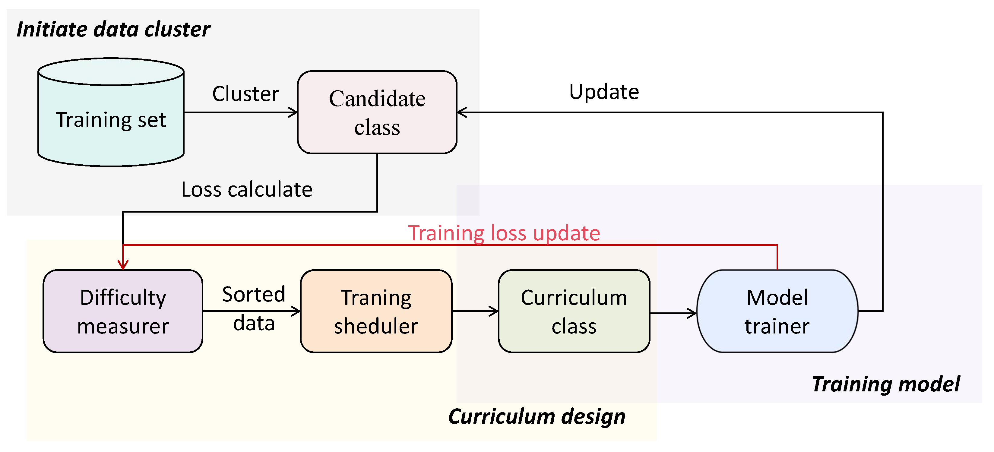
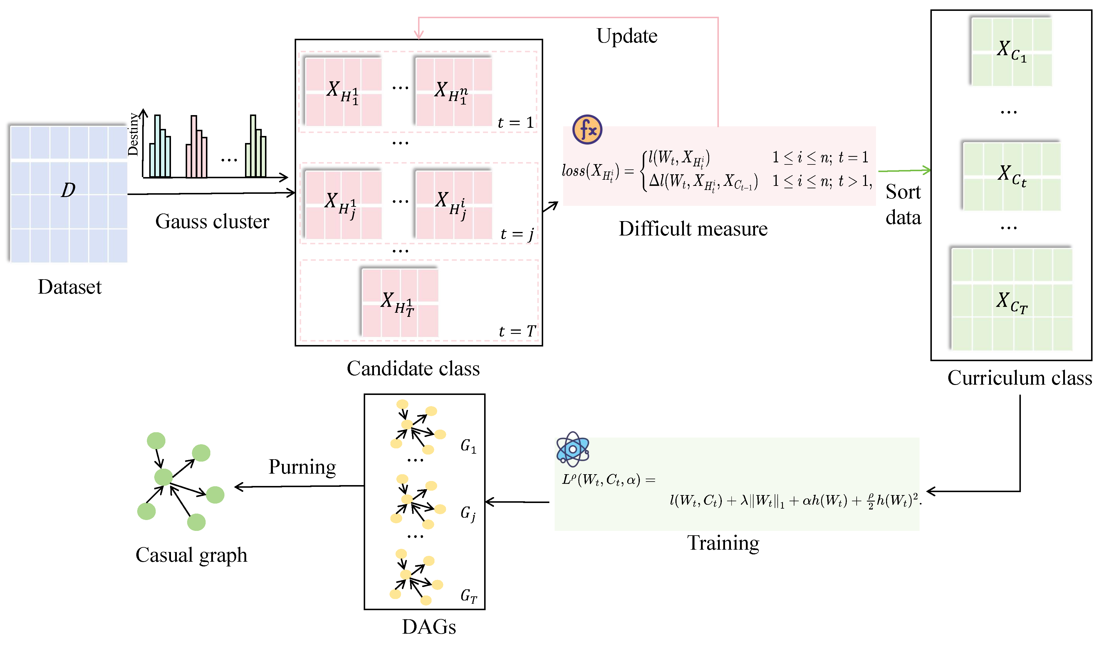
The section begins with constructing a curriculum sample set partitioning model using Gaussian mixture kernel clustering and designing a CSL mechanism based on CL. The constrained problem is then reformulated as an optimization problem using the augmented Lagrangian method (ALM). The final step involves detailing the process of updating causal relationships with dynamic coefficient weighting. The overall framework is illustrated in Figure 2.

4.1. Similarity-Based Dataset Classification

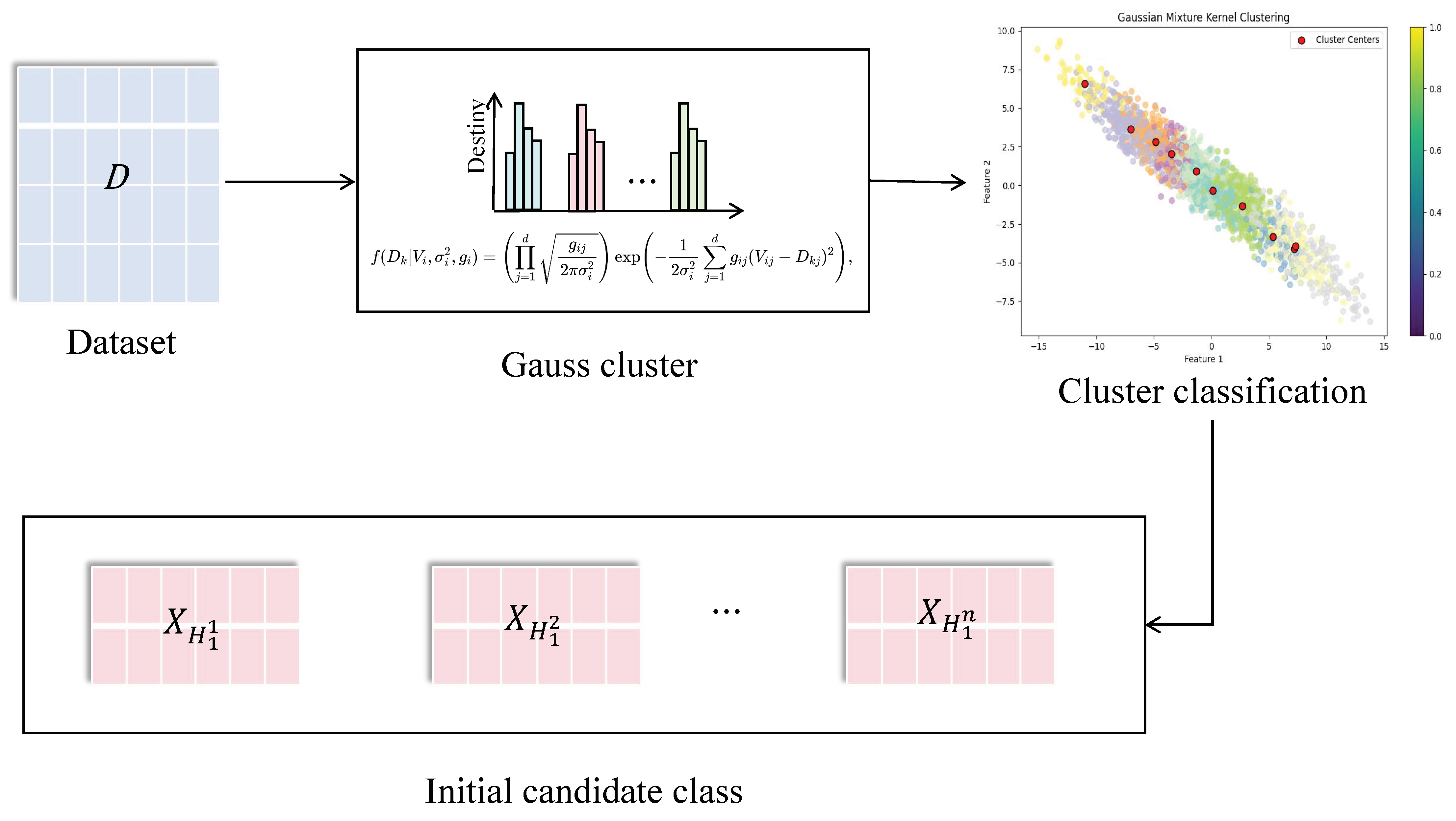
Gaussian distributions have wide practical significance in manufacturing and scientific experiments, as the probability distributions of many random variables can be approximated using Gaussian distributions. For a random variable $X_j$, a Gaussian distribution with mean $\mu$ and variance ${\sigma }^2$ is given by:

$$P\left(X_j\right|\Theta )={\displaystyle \frac{1}{\sqrt{2\pi {\sigma }^2}}}exp\left(-{\displaystyle \frac{{(X_j-\mu )}^2}{2{\sigma }^2}}\right).$$

(4)

Here, $\Theta =\left\{\mu ,{\sigma }^2\right\}$ represents the parameters. $P\left(X_j\right|\Theta )$ describes the probability density function of $X_j$ and indicates how likely different values of $X_j$ are under the Gaussian distribution. Gaussian mixture models offer strong probabilistic interpretations and advantages, such as robustness to noise, and have been widely applied. Leveraging the characteristics of causal learning sample modeling, Gaussian mixture models can cluster the samples that need to be learned, dividing the data sample set into different learning difficulty levels. Assuming the learning sample set is $D=\left\{D_1,D_2,\dots ,D_s\right\}$, where $D_k\in {\mathbb{R}}^d$ (i.e., each sample $D_k$ is a vector of real numbers in d-dimensional space) and each $D_k$ is drawn from a mixture density composed of n Gaussian components, the probability density function is given by:

$$F(D_k;\Theta )=\sum _{i=1}^n{\beta }_{i}f(D_k\mid V_i,{\Sigma }_i),$$

(5)

where ${\beta }_i$, $V_i$, and ${\Sigma }_i$ represent the mixture coefficient, mean vector, and covariance matrix of the $i_{th}$ component, respectively; $f(D_k\mid V_i,{\Sigma }_i)$ is the Gaussian density function of the $i_{th}$ component. Due to the involvement of numerous features in causal sample data that belong to high-dimensional space, traditional clustering methods are difficult to apply directly. Peng et al. [34] introduced information entropy into an extended Gaussian mixture model to address subspace clustering of high-dimensional data, specializing in the covariance matrix of Gaussian vectors:

$${\Sigma }_i={\sigma }_i^{2}diag(g_{i1}^{-1},g_{i2}^{-1},\dots ,g_{id}^{-1}),$$

(6)

where $\mathrm{diag}(g_{i1}^{-1},$$g_{i2}^{-1},\dots ,g_{id}^{-1})$ represents a diagonal matrix with diagonal elements $g_{i1}^{-1},$$g_{i2}^{-1},$$\dots ,g_{id}^{-1}$, where $g_{ij}$ represents the relevance of feature j to cluster i. The term ${\sigma }_i^2$ represents the local variance of cluster i. The probability density function of the $i_{th}$ Gaussian component is:

$$\begin{array}{cc}\hfill f\left(D_k\right|V_i,{\sigma }_i^2,g_i)& =\left(\prod _{j=1}^d\sqrt{{\displaystyle \frac{g_{ij}}{2\pi {\sigma }_i^2}}}\right)exp\left(-{\displaystyle \frac{1}{2{\sigma }_i^2}}\sum _{j=1}^d{g}_{ij}{(V_{ij}-D_{kj})}^2\right),\hfill \end{array}$$

(7)

where $V_{ij}$ is the mean of feature j for the $i_{th}$ cluster, $D_{kj}$ is the $j_{th}$ feature of data k, and $g_{ij}$ adjusts the relevance of feature j for the $i_{th}$ cluster.

By minimizing the Kullback–Leibler (KL) divergence [34] to estimate parameters $\Phi =\left\{{\beta }_i,V_i,{\sigma }_i^2,g_i\mid 1\le i\le n\right\}$, we obtain:

$$\begin{array}{c}\hfill G({\mu }_k,{\beta }_i,V_i,{\sigma }_i^2,g_i)={\displaystyle \frac{1}{n}}\sum _{i=1}^n\sum _{k=1}^s{\mu }_{ik}\left[-log{\beta }_i+\sum _{j=1}^d\left({\displaystyle \frac{g_{ij}}{2{\sigma }_i^2}}{(V_{ij}-D_{kj})}^2-log\sqrt{{\displaystyle \frac{g_{ij}}{2\pi {\sigma }_i^2}}}\right)+log{\mu }_{ik}\right],\end{array}$$

(8)

where ${\mu }_k=\left({\mu }_{1k},{\mu }_{2k},\dots ,{\mu }_{nk}\right)$ is a vector composed of fuzzy membership values.

Building on the research conducted by Peng et al. [34], this work employs the Gaussian mixture kernel clustering method to group causal sample datasets with high-dimensional features. This approach results in curriculum sample sets characterized by high inter-feature similarity, as illustrated in Figure 3. Given that the dataset is modeled using SEM, it is posited that samples with higher similarity tend to exhibit higher quality and have a more significant impact on CSL algorithms. Consequently, the quality of the partitioned curriculum sample sets directly influences the effectiveness of subsequent adaptive training processes.

4.2. The Self-Training Curriculum Framework

CL [35] refers to a series of training criteria over T training steps: $C=〈C_1,C_2,\dots ,C_T〉$, where each criterion $C_t$ involves the reweighting of the target training distribution $P\left(D_i\right)$:

$$C_t\left(D_i\right)\propto O_t\left(D_i\right)P\left(D_i\right)\forall \mathrm{example}{D}_i\in \mathrm{training}\mathrm{set}D,$$

(9)

such that the following three conditions are satisfied:

• The entropy of distributions gradually increases:

  $$H\left(X_{C_t}\right)<H\left(X_{C_{t+1}}\right).$$

  (10)
• The weight for any example increases:

  $$O_t\left(D_i\right)<O_{t+1}\left(D_i\right).$$

  (11)
• The model finally learns all the samples:

  $$C_T\left(D_i\right)=P\left(D_i\right).$$

  (12)

CL is a training strategy for machine learning models that involves using a curriculum to guide the learning process. In Equation (10), it is suggested that the diversity and informativeness of the training set should gradually increase. This means that in later stages, the probability of sampling more challenging examples is increased through reweighting. Equation (11) indicates that more training samples are gradually introduced, thereby enlarging the training set. Finally, Equation (12) signifies that at the end of the process, all sample weights become uniform, and training is conducted on the complete target training set.

Some scholars [36,37] elucidate that CL, from the perspectives of optimization and data distribution, involves progressive learning from “clean” (low-noise) samples to samples with increasing noise. This approach encourages models to focus more on easier data and less on harder data, thereby leading to noise reduction.

Inspired by the CL to mitigate the impact of noise in samples, a CL mechanism is employed to facilitate the adaptive training of these samples. Based on their performance during training, samples are categorized into curriculum samples and candidate samples. Through iterative training, the performance of candidate samples is continually updated, and the next stage of curriculum samples is determined accordingly. Ultimately, the entire set of training samples D is learned.

To achieve adaptive training of curriculum samples, this work designs a curriculum loss function based on acyclicity constraints to evaluate the performance of different samples during the training process. This paper primarily investigates linear SEM and the LS loss $l(W,X)={\displaystyle \frac{1}{2s}}{\parallel X-XW\parallel }_F^2$. Although the results are applicable to any smooth loss function defined on ${\mathbb{R}}^{d\times d}$, extensive research has focused on the statistical properties of the LS loss in scoring DAGs. It has been shown that minimizing the LS loss can recover the true DAG with high probability in finite samples and for high dimensions ($d\gg s$). Thus, for both Gaussian SEM [38,39] and non-Gaussian SEM [40], the LS loss is consistent.

$$\begin{array}{cc}\hfill loss\left(X_{H_t^i}\right)& =\left\{\begin{array}{cc}l(W_t,X_{H_t^i})\hfill & 1\le i\le n;t=1\hfill \\ \Delta l(W_t,X_{H_t^i},X_{C_{t-1}})\hfill & 1\le i\le n;t>1,\hfill \end{array}\right.\hfill \end{array}$$

(13)

where $X_{C_t}$ represents a curriculum sample for the $t_{th}$ stage, and $X_{H_t^i}$ represents the $i_{th}$ candidate sample of the $t_{th}$ stage candidate set. $W_t$ denotes the weighted adjacency matrix of the $t_{th}$ stage.

The loss function for each candidate set in the first curriculum stage is computed using the LS loss $l(W_t,X_{H_t^i})$. In contrast, the difference loss function $\Delta l(W_t,X_{H_t^i},X_{C_{t-1}})$ for the candidate curriculum stages is defined as the difference between the LS loss of the current candidate set and the LS loss of the curriculum sample from the previous stage.

$$l(W_t,X_{H_t^i})={\displaystyle \frac{1}{2s}}{∥X_{H_t^i}-X_{H_t^i}{W}_t∥}_F^2$$

(14)

$$\Delta l(W_t,X_{H_t^i},X_{C_{t-1}})={\displaystyle \frac{1}{2s}}{∥X_{H_t^i}-X_{H_t^i}{W}_t∥}_F^2-l(W_t,X_{C_{t-1}}).$$

(15)

The model adjusts the order of sample learning and updates the curriculum samples and candidate samples based on the losses obtained during the training process. The sample with the minimum loss is selected as the curriculum sample for the next stage, and this sample is removed from the candidate set.

$$\begin{array}{c}\hfill \left\{\begin{array}{cc}{X}_{C_t}=X_{H_t^i}^{\ast }=\underset{i}{min}loss\left(X_{H_t^i}\right)\hfill & 1\le i\le n;1\le t\le T;\hfill \\ X_{H_t}=X_{H_{t-1}}/X_{C_t}\hfill & 1\le i\le n;1\le t\le T;.\hfill \end{array}\right.\end{array}$$

(16)

In each stage, the goal is to learn the causal structure $G_t$ of that stage from the curriculum sample $X_{C_t}$:

$$\begin{array}{c}\hfill \begin{array}{ccc}& \underset{W_t\in R^{d\times d}}{min}& l(W_t,C_t)+\lambda {∥W_t∥}_1\\ & \mathrm{subject}\mathrm{to}& h\left(W_t\right)=0.\end{array}\end{array}$$

(17)

Inspired by NOTEARS, the augmented Lagrangian method (ALM) is employed to transform constrained equations into a series of unconstrained problems. The ALM constructs the scoring function L to optimize the given constrained formulation. The corresponding augmented Lagrangian formula is as follows:

$$L^{\rho }(W_t,C_t,\alpha )=l(W_t,C_t)+\lambda {∥W_t∥}_1+\alpha h\left(W_t\right)+{\displaystyle \frac{\rho }{2}}h{\left(W_t\right)}^2.$$

(18)

When $\rho >0$, it denotes the penalty parameter, and $\alpha$ represents the estimate of the Lagrange multiplier. As $\rho$ tends to infinity, minimizing $L^{\rho }$ necessitates satisfying $h\left(W_t\right)=0$. By gradually increasing $\rho$, the augmented Lagrangian is minimized, and the Lagrange multipliers $\alpha$ are updated to converge to the optimal conditions. In the special case where $\lambda =0$, the nonsmooth term vanishes, and the problem reduces to unconstrained smooth minimization, which can be solved using the L-BFGS approximation algorithm [41]. When $\lambda >0$, the problem can be approximately solved using the PQN method [42].

4.3. Pruning

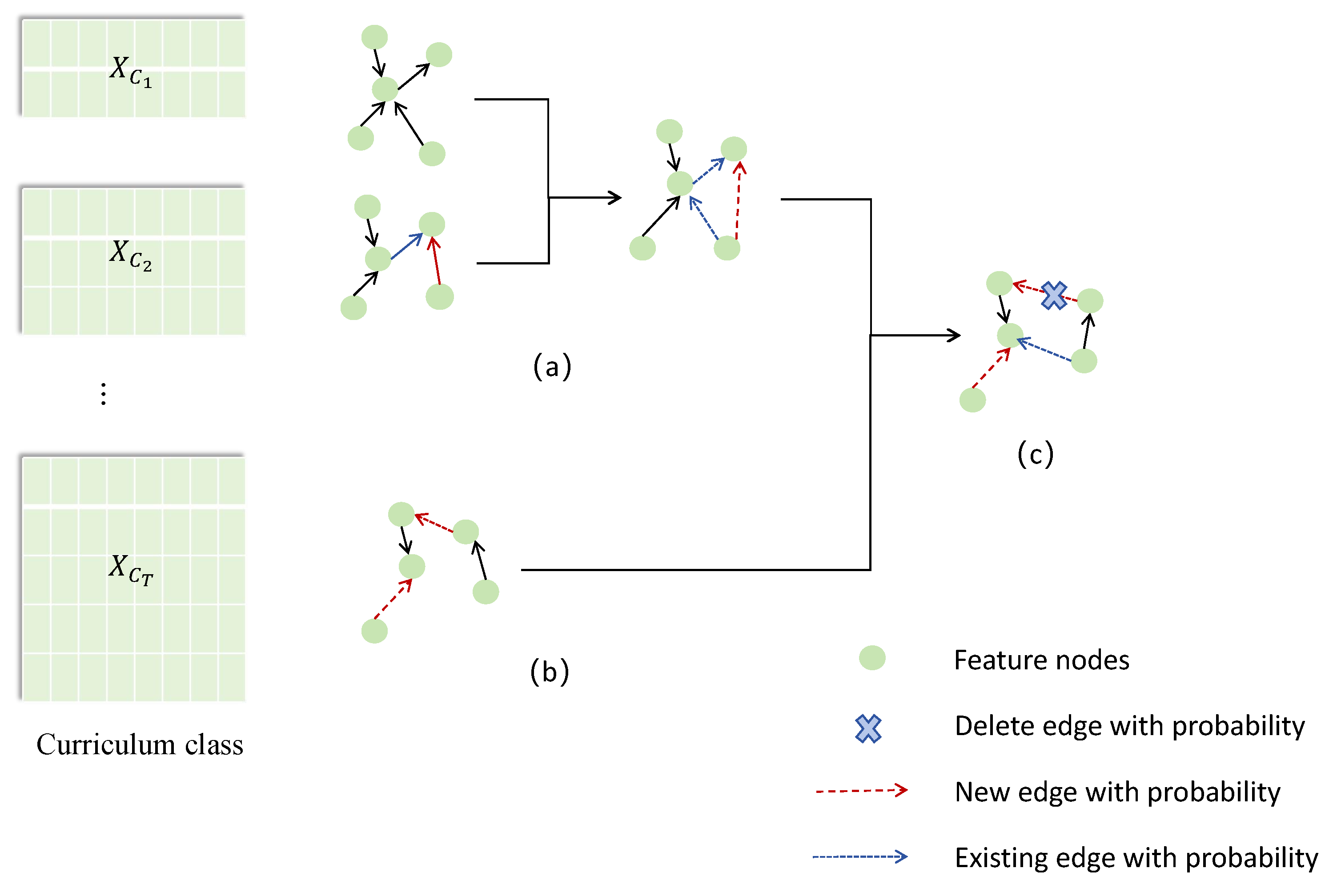
To manage the curriculum iteration process, edge weights are dynamically updated to identify causal edges for generating new samples in subsequent rounds. New causal edges are added to the previously established edge set. After each training update, a probability threshold ($\gamma =0.5$) is applied to determine whether to retain or discard these edges. Figure 4 illustrates this process: (a) shows the causal graph for the first two curriculum stages, (b) represents the $t_{th}$ curriculum stage, and (c) displays the updated result based on (a) and (b). The density of the dashed lines in the figure reflects the probability of the causal edges. To iteratively learn the causal structure across curriculum stages, edge weights and scores are computed.

• Set the edge weights ($B_t$, $M_t$, $N_t$).

  $$\begin{array}{c}\hfill \left\{\begin{array}{c}{B}_t=E_1+E_2+\cdots +E_{C_t}\hfill \\ M_t=E_t-E_{t-1}\hfill \\ N_t=E_{t-1}-E_t,\hfill \end{array}\right.\end{array}$$

  where $E_t$ represents the weight matrix of the edges in the $t_{th}$ stage. Specifically: (1) $B_t$ represents the weight matrix of the edges that always appear in or before the $t_{th}$ stage; (2) $M_t$ represents the weight matrix of new edges appearing in the next curriculum stage; (3) $N_t$ represents the weight matrix of edges that appear in previous curriculum stages and then disappear. The initial curriculum weight is set to ${\displaystyle \frac{t-1}{t}}$, where t is the number of curriculum stages. Subsequent curriculum stages are weighted in decreasing order according to the stage number because the initial curriculum stage has the least data noise, and the learned edges are therefore more reliable.
• Compute score ($S_{\Delta BIC}$). BIC [23] uses the log-likelihood to measure how well the structure fits the data, assuming the samples are independent and identically distributed. The BIC scoring function is given by:

  $$\begin{array}{c}\hfill BIC\left(G\right|D)=\sum _{i=1}^n\sum _{j=1}^{q_i}\sum _{k=1}^{r_i}{m}_{ijk}log{\theta }_{ijk}-{\displaystyle \frac{1}{2}}\sum _{i=1}^n{q}_i(r_i-1)logs.\end{array}$$

  (19)

  where s represents the number of datasets, $m_{ijk}$ represents the probability associated with the $k_{th}$ value when the parent node takes the $j_{th}$ combined value, and ${\sum }_{i=1}^n{q}_i(r_i-1)$ denotes the number of parameters in the network.
  Determine whether the edges in $M_i$ and $N_i$ are retained by calculating the BIC score:

  $$S_{\Delta BIC}=\left\{\begin{array}{cc}1\hfill & BIC\left(G^{\ast }\right|D)-BIC\left(G\right|D)>0\hfill \\ 0\hfill & BIC\left(G^{\ast }\right|D)-BIC\left(G\right|D)\le 0,\hfill \end{array}\right.$$

  (20)

  where G represents the DAG composed of variables $X=\left[X_1,X_2,\dots ,X_d\right]$, and $G^{\ast }$ is the DAG with additional edges from $M_t$ or $N_t$. The term $q_i$ indicates the number of possible values for the parent node of the variable $x_i$, $r_i$ is the number of values of the variable $X_i$, $m_{ijk}$ is the number of samples for which the parent node of $X_i$ takes the value j and $X_i$ takes the value k. The conditional likelihood probability ${\theta }_{ijk}={\displaystyle \frac{m_{ijk}}{m_{ij}}}$, where $0\le {\theta }_{ijk}\le 1$ and ${\sum }_k{\theta }_{ijk}=1$.

Based on the above-mentioned setting, the weight matrix for the $t_{th}$ round, $W_t$, is given by:

$$W_t=B_t+S_{\Delta BIC}{M}_t+S_{\Delta BIC}{N}_t.$$

(21)

4.4. The CL-NOTEARS Algorithm

Based on the analysis above, the CL-NOTEARS algorithm was developed. The algorithm involves three steps: (1) obtaining the initial candidate dataset using a Gaussian mixture kernel clustering method (lines 4–5), (2) computing the loss values for each candidate dataset at various curriculum stages and updating the curriculum dataset based on comparisons (lines 6–15), and (3) updating the weight matrix and iteratively refining the causal structure throughout the CL process (lines 16–17). The pseudocode for the CL-NOTEARS algorithm is provided in Algorithm 1.

Algorithm 1 CL-NOTEARS

Require:     1: $D=\left\{D_1,D_2,\dots ,D_s\right\}$: the dataset;  2: T: the number of curriculum stages;  3: n: the number of Gaussian components.  4: Initialize Initialize weight matrix W with $d\times d$ dimension. Ensure:  DAG: the casual graph  5: Generate an initial set of candidates: $X_{H_1}\Leftarrow Gauss(D,n)$  6: Update weight matrix W using Equation (18) and calculate the loss of candidate datasets using Equation (14)  7: while $t<T$ do  8:     if $t=1$ then  9:          Update the curriculum dataset: $X_{C_1}={min}_{i\in \left[1,n\right]}loss\left(X_{H_1^i}\right)$ 10:         Update the candidate dataset: $X_{H_2}=X_{H_1}/X_{C_1}$ 11:     else 12:         Update weight matrix W using Equation (18) 13:         Calculate the loss of candidate datasets using Equation (15) 14:         Update the curriculum dataset: $X_{C_t}={min}_{i\in \left[1,n\right]}\Delta loss(X_{H_t^i};X_{C_{t-1}})$ 15:         Update the candidate dataset: $X_{H_t}=X_{H_{t-1}}/X_{C_{t-1}}$ 16:     end if 17:     Calculate the score $S_{\Delta BIC}$ 18:     Update causal graph matrix W using Equation (21) 19: end while

5. Experiments

To encompass more general and challenging cases in the CSL scenario, this work addresses the following three research questions:

• $RQ1$: In scenarios involving linear Gaussian (LG) noise and linear non-Gaussian (LN) noise, is the CL-NOTEARS algorithm superior to other models?
• $RQ2$: Are the curriculum mechanism and continual update strategy effective for CSL?
• $RQ3$: In real-world scenarios, can the CL-NOTEARS algorithm still reduce noise in the data and provide a greater advantage?

5.1. General Settings

All the experiments were performed on a computer equipped with an Intel(R) Core(TM) i7-1165G7 CPU at 2.80 GHz and 16 GB of memory, and the compiler environment is PyCharm 2021.1.2.

Datasets Following previous research, we generated six types of synthetic datasets to answer RQ1. For RQ2, we chose four types of LN noise datasets. For RQ3, we utilized real BN data from Sachs.

• Simulated data: The work employed two graph sampling schemes—Erdős–Rényi (ER) and scale-free (SF) [43]—varying across four aspects: the data generation process, number of nodes, edge sparsity, and graph type. The data generation process included LG/LN ANM. For the LG autoregressive model, data were sampled as $X_j=A^T\left(X_{pa\left(j\right)}\right)+N_j$, with independent noise $N_j\sim N(0,I_{d\times d})$. For the LN autoregressive model, the work compared two noise distributions: additive noise $N_j$ from either an exponential or uniform distribution with uniformly sampled variances. Each dataset type was randomly sampled according to ER or SF schemes, and graphs with nodes $(10,30,50)$ and edges $(1.5d,2d,3d)$ were considered.
• Real BN data: The work adopts a real BN dataset—specifically, the Sachs dataset. Sachs is a multivariate proteomic dataset that is widely used in causal discovery. It contains measurements of various proteins and phospholipids found in human immune system cells, including 11 phosphorylated proteins and phospholipids (PKC, PKA, P38, Jnk, Raf, Mek, Erk, Akt, Plcg, PIP2, and PIP3).

The details are shown in

Table 2. Summary of the synthetic and real datasets.

RQ	Dataset	Data Generation Process	Features	Edges	Instances
RQ1	ER-1.5	LG/LN	10/30/50	15/45/75	1000
	ER-2	LG/LN		20/60/100
	ER-3	LG/LN		30/90/150
	SF-1.5	LG/LN	10/30/50	15/45/75	1000
	SF-2	LG/LN		20/60/100
	SF-3	LG/LN		30/90/150
RQ2	ER-2	LG	10/30/50	20/60/100	1000
	ER-3	LG		30/90/150
	SF-2	LG	10/30/50	20/60/100	1000
	SF-3	LG		30/90/150
RQ3	Sachs	Real	11	17	853

ER and SF: graph sampling schemes; instances: number of samples needed for learning.

.

Evaluation index: The work evaluates the quality of learned network structures using the proposed CL-NOTEARS approach through the following measurements:

• Structural Hamming distance (SHD): The SHD is a standard distance used to compare graphs by using their adjacency matrices. It involves calculating the differences between two (binary) adjacency matrices: each missing or non-existent edge in the target graph is considered an error. The smaller the SHD, the fewer incorrect edges are learned, and the better the learning effect.
• True positive rate (TPR): In binary classification, the TPR, also known as sensitivity or recall, measures the proportion of actual positive cases that are correctly identified by a classification model. It is calculated as the number of true positive predictions divided by the sum of true positive and false negative predictions.
• False discovery rate (FDR): The FDR is the ratio of all discoveries that are incorrect or reversed in direction. The FDR helps determine potential false discoveries. The smaller the FDR, the lower the error rate of the learned network structure, and the better the algorithm’s performance.

Using the SHD, TPR, and FDR to measure the benefits of DAG provides a comprehensive evaluation, assessing the network structure, classification accuracy, and performance of feature selection from different perspectives.

Baseline: On the dataset, the work compared CL-NOTEARS against several classical and state-of-the-art methods, including PC [10], NOTEARS [11], DAG-GNN [13], GraN-DAG [32], and DirectLiNGAM [44]. The codes for these baseline methods are available in the pyagrum, case-learn2, and gCastle3 packages. Since PC may learn undirected edges, MCSL [45] was used to treat undirected edges as true edges if the true graph has a directed edge instead.

5.2. Comparison of Linear Models with Gaussian Noise

This section evaluates the proposed methods using LG models with equal-variance Gaussian noise and LiNGAM [46] data models, where the true DAGs are known to be identifiable [47]. The parameters $h\in \{1.5,2,3\}$ and $d\in \{10,30,50\}$ are used to generate the observed data.

In this section, we first present a comparison between CL-NOTEARS and state-of-the-art methods using synthetic datasets generated by linear SEMs.

Table 3. FDR and SHD on ER graphs with linear SEMs, Gaussian noise, and 10/30/50 nodes.

Nodes	Algorithm	ER-2		ER-3
		FDR (↓)	SHD (↓)	FDR (↓)	SHD (↓)
d = 10	PC	0.35 ± 0.11	9.60 ± 2.19	0.49 ± 0.15	19.80 ± 7.66
	NOTEARS	0.06 ± 0.09	3.20 ± 2.68	0.05 ± 0.07	7.40 ± 2.67
	DAG-GNN	0.06±0.08	1.80±2.95	0.08±0.07	3.20 ± 2.86
	Gran-DAG	0.29 ± 0.08	13.80 ± 3.11	0.30 ± 0.07	19.00 ± 1.87
	DirectLiNGAM	0.48 ± 0.19	15.40 ± 8.45	0.49 ± 0.14	21.20 ± 7.63
	Ours	0.00 ± 0.00	1.80 ± 1.30	0.07 ± 0.03	5.60 ± 2.07
d = 30	PC	0.49 ± 0.13	50.60 ± 14.87	0.61 ± 0.07	97.00 ± 10.27
	NOTEARS	0.03 ± 0.03	5.00 ± 1.87	0.14 ± 0.10	26.60 ± 18.01
	DAG-GNN	0.12 ± 0.03	8.80 ± 3.03	0.17 ± 0.11	25.80 ± 16.39
	Gran-DAG	0.38 ± 0.14	53.20 ± 12.38	0.66 ± 0.05	104.60 ± 13.90
	DirectLiNGAM	0.71 ± 0.09	72.40 ± 16.40	0.69 ± 0.04	130.20 ± 16.47
	Ours	0.00 ± 0.01	2.60 ± 0.89	0.02 ± 0.02	9.00 ± 2.83
d = 50	PC	0.42 ± 0.14	65.80 ± 28.42	0.64 ± 0.09	169.60 ± 19.82
	NOTEARS	0.08 ± 0.07	16.00 ± 9.17	0.11 ± 0.09	34.80 ± 22.87
	DAG-GNN	0.09 ± 0.07	16.00 ± 13.69	0.12 ± 0.03	32.20 ± 10.13
	Gran-DAG	0.49 ± 0.17	106.00 ± 21.71	0.71 ± 0.05	194.40 ± 28.16
	DirectLiNGAM	0.70 ± 0.07	149.60 ± 51.16	0.77 ± 0.06	254.60 ± 23.27
	Ours	0.02 ± 0.03	8.00 ± 4.41	0.03 ± 0.02	14.40 ± 7.02

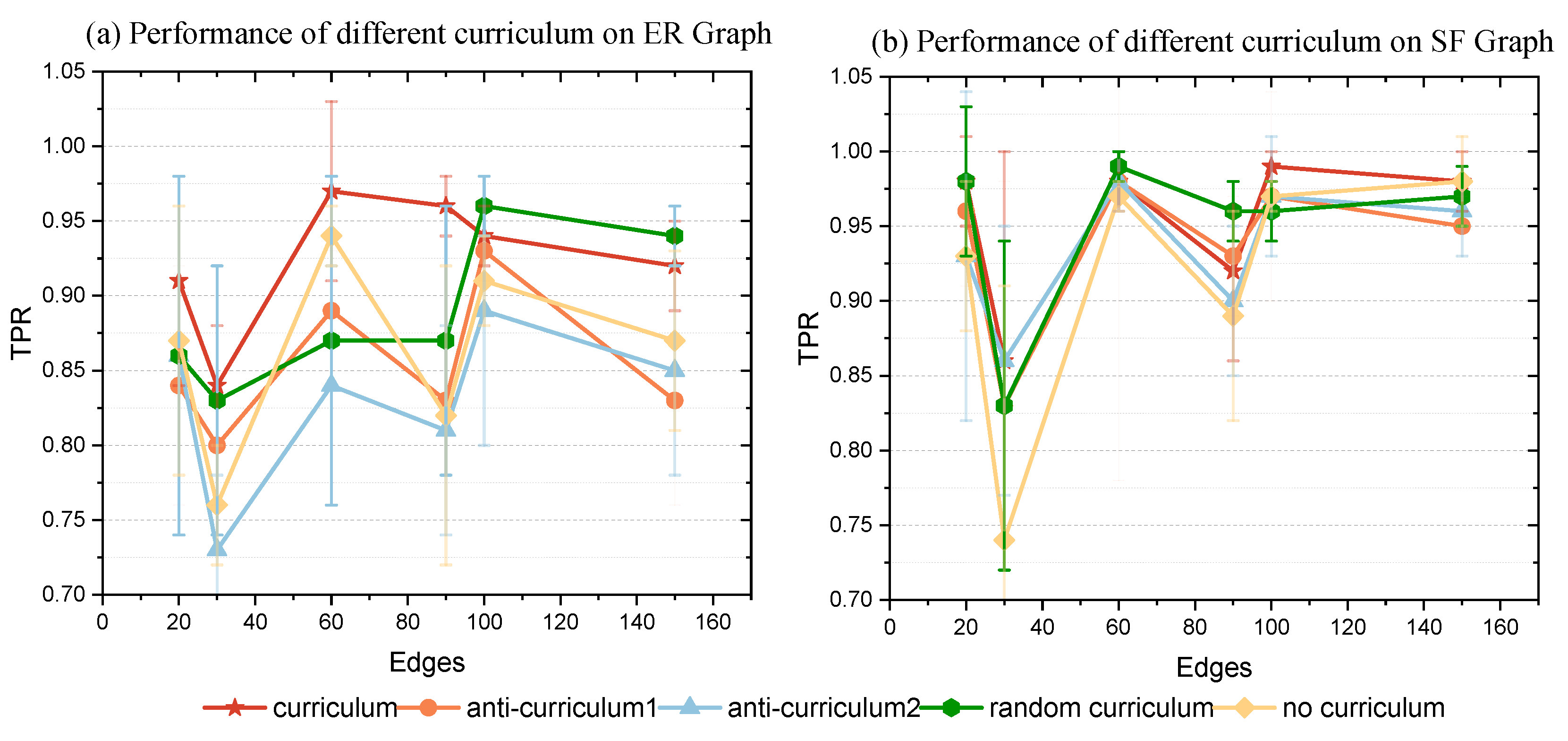
The bold values represent the optimal values within the methods, with the values following ± indicating the standard deviation of the method’s performance across five iterations of training.

and

Table 4. FDR and SHD on SF graphs with linear SEMs, Gaussian noise, and 10/30/50 nodes.

Nodes	Algorithm	SF-2		SF-3
		FDR (↓)	SHD (↓)	FDR (↓)	SHD (↓)
d = 10	PC	0.34 ± 0.14	9.00 ± 3.55	0.50 ± 0.10	18.00 ± 3.24
	NOTEARS	0.07 ± 0.07	0.60 ± 1.14	0.11 ± 0.11	7.40 ± 5.13
	DAG-GNN	0.02 ± 0.03	0.60 ± 0.89	0.06 ± 0.07	2.60 ± 2.70
	Gran-DAG	0.26 ± 0.19	13.20 ± 2.17	0.22 ± 0.18	16.20 ± 3.96
	DirectLiNGAM	0.58 ± 0.28	16.00 ± 8.25	0.60 ± 0.04	20.80 ± 1.10
	Ours	0.00 ± 0.00	0.40 ± 0.55	0.10 ± 0.08	6.80 ± 3.56
d = 30	PC	0.54 ± 0.09	52.00 ± 6.43	0.60 ± 0.07	84.40 ± 6.73
	NOTEARS	0.01 ± 0.01	2.00 ± 1.22	0.09 ± 0.11	16.40 ± 15.26
	DAG-GNN	0.19 ± 0.10	18.80 ± 10.85	0.18 ± 0.05	23.80 ± 6.14
	Gran-DAG	0.34 ± 0.21	52.20 ± 8.04	0.46 ± 0.18	80.20 ± 10.18
	DirectLiNGAM	0.66 ± 0.07	70.80 ± 8.93	0.71 ± 0.08	120.60 ± 15.53
	Ours	0.01 ± 0.01	1.20 ± 1.22	0.08 ± 0.08	13.00 ± 11.55
d = 50	PC	0.52 ± 0.11	98.10 ± 41.26	0.65 ± 0.10	154.40 ± 18.39
	NOTEARS	0.01 ± 0.01	3.00 ± 1.58	0.01 ± 0.01	4.20 ± 4.15
	DAG-GNN	0.23 ± 0.10	38.60 ± 15.61	0.20 ± 0.10	55.40 ± 23.09
	Gran-DAG	0.42 ± 0.16	92.60 ± 8.76	0.60 ± 0.23	162.40 ± 25.59
	DirectLiNGAM	0.69 ± 0.02	140.75 ± 2.87	0.76 ± 0.07	238.20 ± 30.07
	Ours	0.01 ± 0.01	1.40 ± 1.14	0.00 ± 0.00	3.80 ± 2.77

The bold values represent the optimal values within the methods. The values following ± indicate the standard deviation of the method’s performance across five iterations of training.

show the variations in FDR and SHD for the CL-NOTEARS model on ER- and SF-sampled datasets of LG ANM, respectively. Figure 5 illustrates the TPR performance of CL-NOTEARS across these six classes of datasets. The following observations can be made: (1) PC performs poorly due to the dense graphs in the generated data. (2) Both NOTEARS and DAG-GNN exhibit high performance in causal discovery. (3) GraN-DAG performs worse because it uses a two-layer feedforward neural network to model causal relationships, which limits its ability to effectively learn the ideal causal structures. (4) When $d=10$, the CL-NOTEARS algorithm does not show significant superiority over DAG-GNN, whereas when $d=50$, CL-NOTEARS demonstrates strong advantages. Moreover, with the same number of nodes, CL-NOTEARS exhibits increasing superiority as the number of edges grows. This is because with the increase in both nodes and edges, the network becomes more complex, introducing relatively more noise into the sampled datasets. CL-NOTEARS leverages the curriculum-grained framework for noise reduction, allowing it to learn relatively accurate causal structures even in higher-noise datasets, thus demonstrating significant advantages. (5) For each node-size dataset, the FDR value of the CL-NOTEARS algorithm ranges between 0 and 0.01, confirming that the CL framework effectively mitigates the impact of data noise and reduces the occurrence of erroneous edges.

5.3. Comparison of Linear Models with Non-Gaussian Noise

LN data models were evaluated with noise types set to exponential and uniform distributions. For both cases, $h\in \left\{2,3\right\}$ and $d\in \left\{10,30\right\}$, generating observational data with 2000 instances per dataset. Four causal learning algorithms were compared: the traditional CB method PC algorithm, the GB methods DAG-GNN and GraN-DAG, and the NOTEARS algorithm.

For ER and SF graphs of SEM with LN noise, the experimental results are presented in

Table 5. FDR and SHD on ER/SF graphs with linear SEMs, exponential noise, and 10/30 nodes.

Nodes	Algorithm	ER-2		ER-3
		TPR (↑)	SHD (↓)	TPR (↑)	SHD (↓)
d = 10	PC	0.59 ± 0.20	12.60 ± 9.94	0.35 ± 0.09	21.80 ± 4.82
	NOTEARS	0.89 ± 0.11	2.40 ± 2.07	0.79 ± 0.04	7.20 ± 0.84
	DAG-GNN	0.94 ± 0.10	3.60 ± 5.13	0.94 ± 0.06	5.20 ± 3.71
	Gran-DAG	0.22 ± 0.15	13.40 ± 6.66	0.11 ± 0.08	24.20 ± 5.64
	Ours	0.86 ± 0.08	3.00 ± 1.22	0.73 ± 0.09	9.40 ± 2.88
d = 30	PC	0.51 ± 0.08	47.00 ± 11.77	0.27 ± 0.03	90.80 ± 8.23
	NOTEARS	0.91 ± 0.30	7.60 ± 3.29	0.89 ± 0.05	12.00 ± 7.59
	DAG-GNN	0.94 ± 0.05	16.60 ± 13.52	0.88 ± 0.06	42.00 ± 26.41
	Gran-DAG	0.11 ± 0.04	53.80 ± 8.89	0.15 ± 0.05	83.80 ± 7.29
	Ours	0.94 ± 0.05	5.40 ± 4.51	0.91 ± 0.04	10.40 ± 5.27
		SF-2		SF-3
		TPR (↑)	SHD (↓)	TPR (↑)	SHD (↓)
d = 10	PC	0.61 ± 0.17	8.40 ± 2.79	0.41 ± 0.14	16.80 ± 0.35
	NOTEARS	0.85 ± 0.22	3.80 ± 5.50	0.82 ± 0.11	6.20 ± 3.12
	DAG-GNN	0.98 ± 0.03	0.20 ± 0.45	0.97 ± 0.04	1.60 ± 2.08
	Gran-DAG	0.44 ± 0.14	12.20 ± 3.56	0.35 ± 0.13	17.20 ± 1.64
	Ours	0.91 ± 0.06	1.80 ± 1.40	0.83 ± 0.07	4.20 ± 1.64
d = 30	PC	0.53 ± 0.12	43.00 ± 13.56	0.35 ± 0.06	76.60 ± 8.14
	NOTEARS	0.97 ± 0.02	1.40 ± 1.14	0.93 ± 0.07	8.60 ± 10.45
	DAG-GNN	0.87 ± 0.08	15.00 ± 23.10	0.84 ± 0.11	39.20 ± 19.87
	Gran-DAG	0.31 ± 0.07	49.40 ± 6.47	0.22 ± 0.04	89.40 ± 15.54
	Ours	0.98 ± 0.02	1.20 ± 1.10	0.95 ± 0.01	5.40 ± 1.67

The bold values represent the optimal values within the methods, with the values following ± indicating the standard deviation of the method’s performance across five iterations of training.

and

Table 6. FDR and SHD on ER/SF graphs with linear SEMs, uniform noise, and 10/30 nodes.

Nodes	Algorithms	ER-2		ER-3
		TPR (↑)	SHD (↓)	TPR (↑)	SHD (↓)
d = 10	PC	0.48 ± 0.20	16.20 ± 6.50	0.44 ± 0.15	19.20 ± 6.10
	NOTEARS	0.61 ± 0.11	8.80 ± 2.86	0.48 ± 0.06	17.00 ± 2.65
	DAG-GNN	0.92 ± 0.11	1.80 ± 2.49	0.86 ± 0.12	6.00 ± 4.31
	Gran-DAG	0.48 ± 0.18	10.40 ± 2.50	0.35 ± 0.20	21.60 ± 7.16
	Ours	0.68 ± 0.08	8.00 ± 1.22	0.51 ± 0.05	15.00 ± 2.00
d = 30	PC	0.50 ± 0.13	48.80 ± 16.12	0.27 ± 0.06	92.00 ± 10.75
	NOTEARS	0.76 ± 0.05	14.80 ± 3.27	0.61 ± 0.06	48.80 ± 7.26
	DAG-GNN	0.91 ± 0.06	11.20 ± 5.40	0.94 ± 0.04	16.00 ± 10.77
	Gran-DAG	0.28 ± 0.08	48.40 ± 12.68	0.22 ± 0.11	95.60 ± 30.14
	Ours	0.80 ± 0.03	13.60 ± 0.81	0.73 ± 0.04	30.20 ± 4.87
		SF-2		SF-3
		TPR (↑)	SHD (↓)	TPR (↑)	SHD (↓)
d = 10	PC	0.58 ± 0.05	9.20 ± 0.84	0.39 ± 0.09	17.40 ± 1.95
	NOTEARS	0.76 ± 0.18	4.00 ± 3.09	0.76 ± 0.09	6.40 ± 2.19
	DAG-GNN	0.86 ± 0.14	4.40 ± 4.39	0.98 ± 0.04	0.80 ± 1.4
	Gran-DAG	0.44 ± 0.26	11.20 ± 4.44	0.30 ± 0.09	20.40 ± 3.29
	Ours	0.85 ± 0.08	3.00 ± 1.87	0.78 ± 0.11	6.00 ± 2.23
d = 30	PC	0.52 ± 0.11	44.80 ± 13.95	0.31 ± 0.07	79.80 ± 8.41
	NOTEARS	0.82 ± 0.12	12.40 ± 9.34	0.79 ± 0.08	21.40 ± 8.56
	DAG-GNN	0.91 ± 0.09	11.40 ± 10.36	0.84 ± 0.12	33.00 ± 20.96
	Gran-DAG	0.25 ± 0.07	63.00 ± 15.87	0.21 ± 0.05	80.40 ± 16.02
	Ours	0.89 ± 0.02	6.60 ± 1.34	0.85 ± 0.07	14.80 ± 6.50

The bold values represent the optimal values within the methods, with the values following ± indicating the standard deviation of the method’s performance across five iterations of training.

. The results show that DAG-GNN significantly outperforms the other algorithms. This is due to its ability to capture complex interactions and nonlinear transformations among features in linear models under non-Gaussian noise. In contrast, the CL-NOTEARS model performs less effectively with non-Gaussian noise compared to Gaussian noise. This is because the initial partitioning of the CL-NOTEARS algorithm relies on Gaussian mixture models, making it sensitive to the clustering effects of non-Gaussian noise.

5.4. The Effect of Different Curriculum Difficulty Levels on the Learning Process

This work revisited Bengio’s proposed CL prototype model, as highlighted in the literature discussion in Section 5. It explored various challenges in the curriculum mechanism by considering three cases:

• Curriculum mechanism: a basic setup that progresses from easy to difficult, where learning begins with simple sample examples and gradually advances to more complex ones.
• Anti-curriculum mechanism: under anti-curriculum conditions, two mechanisms based on the original CL-NOTEARS model architecture were designed: (1) initially learning from difficult sample tasks and then transitioning from simple to complex samples in subsequent learning phases and (2) learning progresses from complex samples to simple samples throughout the entire process.
• Random curriculum mechanism: learning from samples of varying difficulties selected randomly.

The specific design is illustrated in Figure 6.

Based on these three curriculum mechanisms, the CL-NOTEARS algorithm was integrated and compared with the NOTEARS algorithm, which lacks a curriculum mechanism. Observational data were generated with $h=\{2,3\}$ and $d=\{10,30,50\}$, with each dataset containing 2000 instances.

Table 7. FDR and SHD of different curriculum mechanisms on ER/SF graph with linear SEM and 10/30/50 nodes.

Nodes	Algorithm	ER-2		ER-3
		FDR (↓)	SHD (↓)	FDR (↓)	SHD (↓)
d = 10	Curriculum	0.03 ± 0.05	3.00 ± 2.31	0.07 ± 0.03	6.80 ± 2.49
	Anti-curriculum 1	0.07 ± 0.07	3.80 ± 2.32	0.06 ± 0.06	7.00 ± 2.34
	Anti-curriculum 2	0.12 ± 0.11	3.80 ± 3.12	0.13 ± 0.05	10.60 ± 2.51
	Random curriculum	0.05 ± 0.07	3.20 ± 3.12	0.06 ± 0.04	5.60 ± 2.97
	No curriculum	0.06 ± 0.09	3.20 ± 2.68	0.05 ± 0.07	7.40 ± 2.67
d = 30	Curriculum	0.00 ± 0.01	2.60 ± 0.89	0.02 ± 0.02	9.00 ± 2.83
	Anti-curriculum 1	0.05 ± 0.02	8.60 ± 3.5	0.11 ± 0.06	23.40 ± 9.72
	Anti-curriculum 2	0.14 ± 0.11	16.80 ± 11.8	0.13 ± 0.08	26.00 ± 11.58
	Random curriculum	0.09 ± 0.14	12.60 ± 15.32	0.13 ± 0.12	22.40 ± 18.02
	No curriculum	0.03 ± 0.03	5.00 ± 1.87	0.14 ± 0.10	26.60 ± 18.01
d = 50	Curriculum	0.02 ± 0.03	8.00 ± 4.41	0.03 ± 0.02	14.40 ± 7.02
	Anti-curriculum 1	0.04 ± 0.02	11.20 ± 4.08	0.14 ± 0.12	45.40 ± 31.30
	Anti-curriculum 2	0.09 ± 0.09	18.80 ± 15.34	0.11 ± 0.06	35.80 ± 15.89
	Random curriculum	0.04 ± 0.04	7.60 ± 5.98	0.02 ± 0.02	11.00 ± 5.24
	No curriculum	0.08 ± 0.07	16.00 ± 9.17	0.11 ± 0.09	34.80 ± 22.87
		SF-2		SF-3
		FDR (↓)	SHD (↓)	FDR (↓)	SHD (↓)
d = 10	Curriculum	0.00 ± 0.00	0.40 ± 0.55	0.10 ± 0.08	6.80 ± 3.56
	Anti-curriculum 1	0.02 ± 0.05	0.80 ± 1.30	0.10 ± 0.15	5.80 ± 5.54
	Anti-curriculum 2	0.01 ± 0.02	1.40 ± 1.67	0.07 ± 0.13	5.00 ± 4.53
	Random curriculum	0.01 ± 0.02	0.60 ± 1.34	0.05 ± 0.05	4.40 ± 2.97
	No Curriculum	0.07 ± 0.07	0.60 ± 1.14	0.11 ± 0.11	7.40 ± 5.13
d = 30	Curriculum	0.01 ± 0.01	1.20 ± 1.22	0.08 ± 0.08	13.00 ± 11.55
	Anti-curriculum 1	0.01 ± 0.02	1.20 ± 1.78	0.06 ± 0.05	9.80 ± 6.46
	Anti-curriculum 2	0.01 ± 0.02	1.20 ± 1.78	0.10 ± 0.06	16.00 ± 8.71
	Random curriculum	0.01 ± 0.01	0.40 ± 0.55	0.02 ± 0.01	4.00 ± 2.00
	No Curriculum	0.01 ± 0.01	2.00 ± 1.22	0.09 ± 0.11	16.40 ± 15.26
d = 50	Curriculum	0.01 ± 0.01	0.98 ± 0.02	0.00 ± 0.00	3.80 ± 2.77
	Anti-curriculum 1	0.03 ± 0.06	5.80 ± 11.86	0.04 ± 0.05	12.60 ± 9.53
	Anti-curriculum 2	0.05 ± 0.09	6.60 ± 11.99	0.04 ± 0.04	12.00 ± 9.00
	Random curriculum	0.01 ± 0.01	1.40 ± 1.52	0.01 ± 0.01	6.00 ± 4.06
	No Curriculum	0.01 ± 0.01	3.00 ± 1.58	0.01 ± 0.01	4.20 ± 4.15

The bold values represent the optimal values within the methods, with the values following ± indicating the standard deviation of the method’s performance across five iterations of training. ¹ Description of anti-curriculum method 1. ² Description of anti-curriculum method 2.

shows the FDR and SHD performances for different curriculum mechanisms on the datasets, while Figure 7 visually demonstrates the causal relationships captured by the different curriculum mechanisms. Observations indicate: (1) curriculum ≥ anti-curriculum 1 ≥ anti-curriculum 2; the first anti-curriculum mechanism performs better than the second one, as it only changes the difficulty of the initial learning task, resulting in less disturbance from noise compared to the second mechanism. (2) The random curriculum mechanism exhibits more variable performance compared to the curriculum mechanism. Figure 7 shows that the errors associated with the random curriculum mechanism are significantly larger and essentially encompass the range of errors found with the curriculum mechanism. This variability is due to the random sampling approach, which introduces randomness into the learning process, occasionally leading to better outcomes than those achieved with the curriculum mechanism.

5.5. The Impact of the Number of Curriculum Stages on Algorithms

The number of curriculum stages in the algorithm influences the size of the learning sample set at different stages, which in turn affects the accuracy of separating the sample set at various noise levels. To investigate the effect of the curriculum stage size on the algorithm, four different sizes were considered: $T=\{5,10,15,20\}$. Observation data were generated with $h=\left\{2,3\right\}$ and $d=\left\{10,30\right\}$. The dataset was randomly sampled using the ER scheme to create a real DAG consisting of 2000 sample instances. Evaluation metrics included TPR and SHD. Each experimental result was averaged over five sets of data, and the results are summarized in

Table 8. TPR and SHD of different curriculum stages on an ER graph with linear SEM and 10/30 nodes.

Nodes	Curriculum Stages	ER-2		ER-3
		TPR (↑)	SHD (↓)	TPR (↑)	SHD (↓)
d = 10	T = 5	0.85 ± 0.09	4.00 ± 2.45	0.72 ± 0.12	10.00 ± 4.47
	T = 10	0.90 ± 0.07	3.00 ± 2.31	0.81 ± 0.06	6.80 ± 2.49
	T = 15	0.76 ± 0.08	6.20 ± 2.86	0.63 ± 0.09	12.60 ± 4.04
	T = 20	0.82 ± 0.10	5.40 ± 3.21	0.63 ± 0.10	13.00 ± 3.39
d = 30	T = 5	0.87 ± 0.05	10.20 ± 4.21	0.81 ± 0.12	30.20 ± 20.22
	T = 10	0.97 ± 0.06	6.40 ± 5.68	0.96 ± 0.02	12.20 ± 3.42
	T = 15	0.84 ± 0.09	17.40 ± 11.65	0.80 ± 0.08	32.00 ± 14.97
	T = 20	0.85 ± 0.05	15.20 ± 7.53	0.81 ± 0.13	29.40 ± 17.34

The bold values represent the optimal values within the methods, with the values following ± indicating the standard deviation of the method’s performance across five iterations of training.

.

It can be seen from Table 8 that the best performance occurs when the number of curriculum stages is 10. Based on the experimental data, we speculate that if the number of curriculum stages is too large, sample division becomes too fine, making it difficult for the algorithm to differentiate between noise and signals in small samples, which results in poor learning performance. Conversely, if the number of curriculum stages is too small, the sample division is too coarse, and the sample set learned in each stage becomes noisy, and the model fails to balance noise differences effectively. Therefore, when dividing curriculum stages, the size of each stage should be adjusted based on the size of the sample set for that stage.

5.6. Real Data

The Sachs dataset [48], which contains 11 nodes and 17 edges, is widely used in the study of graph models. The expression levels of proteins and phospholipids in this dataset can be used to uncover the underlying protein signaling network. This dataset is a common benchmark in graph modeling, and its experimental annotations are widely accepted by the biological community and encompass both observational and interventional aspects. The observational dataset includes $m=853$ samples and is used to discover causal structures. The work also uses Gaussian process regression to simulate causality and to calculate the score. Since the real network structure is sparse, the SHD of an empty graph can be as low as 17. Comparing the best available algorithms, detailed results of the estimated graphs constructed by the different algorithms are shown in

Table 9. Comparison of different algorithms on the Sachs network.

	NOTEARS	DAG-GNN	Gran-DAG	CL-NOTEARS
Total Edges	20	15	10	13
Correct Edges	6	6	5	6
SHD	19	16	13	13

The bold values represent the optimal values within the methods.

. This includes the total number of edges, the number of correct edges, and the SHD. The PC algorithm, which outputs many undirected edges, is not included in this comparison.

As shown in Table 9, the CL-NOTEARS algorithm demonstrates a significant advantage over other methods, achieving an optimal value of 13. Although the CL-NOTEARS algorithm identifies the same number of correct edges as the NOTEARS algorithm, it exhibits a substantial reduction in the SHD and a marked decrease in the number of erroneous edges. This improvement is attributed to the CL framework, which mitigates the impact of data noise on the algorithm, thereby significantly reducing the number of erroneous edges detected.

6. Conclusions

The work proposes a continuous optimization algorithm based on the CL framework, called CL-NOTEARS. This algorithm addresses the challenge of sample learning by evaluating the performance of the loss function on different sample sets, transforming the combinatorial optimization problem in discrete space into a numerical continuous optimization problem within various curriculum frameworks. Additionally, a dynamic weight adaptation method is employed for different curriculum stages to adjust the learning network’s structure. This reduces the impact of data noise on CSL algorithms and helps prevent the algorithm from falling into local optima. Extensive experiments on various synthetic datasets have demonstrated the effectiveness of the proposed approach.

In the future, we plan to further investigate batch adaptive mechanisms and noise-check evaluation methods in CSL to further reduce the impact of data noise on the algorithm and explore the universality of this mechanism for other algorithms.

References

1. Squires, C. Causal Structure Learning: A Combinatorial Perspective. Found. Comput. Math. 2023, 23, 1781–1815. [Google Scholar] [CrossRef] [PubMed]
2. Zhou, F.; He, K.; Ni, Y. Causal discovery with heterogeneous observational data. In Proceedings of the Thirty-Eighth Conference on Uncertainty in Artificial Intelligence, Eindhoven, The Netherlands, 1–5 August 2022; Volume 180, pp. 2383–2393. [Google Scholar]
3. Wang, L.; Chignell, M.; Jiang, H.; Lokuge, S.; Mason, G.; Fotinos, K.; Katzman, M. Discovering the Causal Structure of the Hamilton Rating Scale for Depression Using Causal Discovery. In Proceedings of the 2021 IEEE EMBS International Conference on Biomedical and Health Informatics (BHI), Athens, Greece, 27–30 July 2021; pp. 1–4. [Google Scholar] [CrossRef]
4. Wan, C.X. Financial causal sentence recognition based on BERT-CNN text classification. J. Supercomput. 2022, 78, 6503–6527. [Google Scholar] [CrossRef]
5. Umesh Kumar Lilhore, M.P.; Algarni, A.D. Hybrid Model for Detection of Cervical Cancer Using Causal Analysis and Machine Learning Techniques. Comput. Math. Methods Med. 2022, 2022, 4688327. [Google Scholar] [CrossRef]
6. Xu, J.; Wang, Q.; Zhou, J.; Zhou, H.; Chen, J. Improved Bayesian network-based for fault diagnosis of air conditioner system. Int. J. Metrol. Qual. Eng. 2023, 14, 10. [Google Scholar] [CrossRef]
7. Qin, W.; Zhang, H.; Hong, R.; Lim, E.P.; Sun, Q. Causal Interventional Training for Image Recognition. IEEE Trans. Multimed. 2023, 25, 1033–1044. [Google Scholar] [CrossRef]
8. Chickering, D.M. Learning Bayesian networks is NP-complete. Learn. Data Artif. Intell. Stat. V 1996, 112, 121–130. [Google Scholar] [CrossRef]
9. Neuberg, L.G. CAUSALITY: MODELS, REASONING, AND INFERENCE, by Judea Pearl, Cambridge University Press, 2000. Econom. Theory 2003, 19, 675–685. [Google Scholar] [CrossRef]
10. Spirtes, P.; Glymour, C.; Scheines, R. Causation, Prediction, and Search; The MIT Press: Cambridge, MA, USA, 2001. [Google Scholar] [CrossRef]
11. Zheng, X.; Aragam, B.; Ravikumar, P.; Xing, E.P. DAGs with NO TEARS: Continuous optimization for structure learning. In Proceedings of the 32nd International Conference on Neural Information Processing Systems, NIPS’18, Red Hook, NY, USA, 2–8 December 2018; pp. 9492–9503. [Google Scholar]
12. Ng, I.; Zhu, S.; Chen, Z.; Fang, Z. A Graph Autoencoder Approach to Causal Structure Learning. arXiv 2019, arXiv:1911.07420. [Google Scholar]
13. Yu, Y.; Chen, J.; Gao, T.; Yu, M. DAG-GNN: DAG Structure Learning with Graph Neural Networks. In Proceedings of the 36th International Conference on Machine Learning, Long Beach, CA, USA, 9–15 June 2019; Proceedings of Machine Learning Research. Chaudhuri, K., Salakhutdinov, R., Eds.; Curran Associates, Inc.: Mount Kisco, NY, USA, 2019; Volume 97, pp. 7154–7163. [Google Scholar]
14. Bengio, Y.; Louradour, J.; Collobert, R.; Weston, J. Curriculum learning. In Proceedings of the 26th Annual International Conference on Machine Learning, ICML’09, New York, NY, USA, 14–18 June 2009; pp. 41–48. [Google Scholar] [CrossRef]
15. Platanios, E.A.; Stretcu, O.; Neubig, G.; Poczos, B.; Mitchell, T. Competence-based Curriculum Learning for Neural Machine Translation. In Proceedings of the 2019 Conference of the North American Chapter of the Association for Computational Linguistics: Human Language Technologies, Volume 1 (Long and Short Papers); Burstein, J., Doran, C., Solorio, T., Eds.; Association for Computational Linguistics: Stroudsburg, PA, USA, 2019; pp. 1162–1172. [Google Scholar] [CrossRef]
16. Tsamardinos, I.; Aliferis, C.; Statnikov, A. Algorithms for Large Scale Markov Blanket Discovery. FLAIRS 2003, 2, 376–381. [Google Scholar]
17. Spirtes, P.; Glymour, C.; Scheines, R. From probability to causality. Philos. Stud. 1991, 64, 1–36. [Google Scholar] [CrossRef]
18. Li, Y.; Yang, Y.; Zhu, X.; Yang, W. From probability to causality. Wuhan Univ. J. Nat. Sci. 2015, 20, 214–220. [Google Scholar] [CrossRef]
19. Colombo, D.; Maathuis, M.H. Order-Independent Constraint-Based Causal Structure Learning. J. Mach. Learn. Res. 2014, 15, 3741–3782. [Google Scholar]
20. Le, T.D.; Hoang, T.; Li, J.; Liu, L.; Liu, H.; Hu, S. A fast PC algorithm for high dimensional causal discovery with multi-core PCs. IEEE/ACM Trans. Comput. Biol. Bioinform. 2016, 16, 1483–1495. [Google Scholar] [CrossRef]
21. Sun, X.; Janzing, D.; Schölkopf, B.; Fukumizu, K. A kernel-based causal learning algorithm. In Proceedings of the 24th International Conference on Machine Learning, ICML’07, Corvallis, OR, USA, 20–24 June 2007; pp. 855–862. [Google Scholar] [CrossRef]
22. Zhang, K.; Peters, J.; Janzing, D.; Schölkopf, B. Kernel-based conditional independence test and application in causal discovery. In Proceedings of the Twenty-Seventh Conference on Uncertainty in Artificial Intelligence, UAI’11, Arlington, Barcelona, Spain, 14–17 July 2011; pp. 804–813. [Google Scholar]
23. David Heckerman, D.G.; Chickering, D.M. Learning Bayesian networks: The combination of knowledge and statistical data. Mach. Learn. 1995, 20, 197–243. [Google Scholar] [CrossRef]
24. Hiramatsu, K.; Matsumiya, Y.; Kitada, S. Introduction of Suitable Stock-recruitment Relationship by a Comparison of Statistical Models. Fish. Sci. 1994, 60, 411–414. [Google Scholar] [CrossRef]
25. Bouckaert, R.R. Probalistic Network Construction Using the Minimum Description Length Principle. In Proceedings of the European Conference on Symbolic and Quantitative Approaches to Reasoning and Uncertainty, ECSQARU ’93, Granada, Spain, 8–10 November 1993; pp. 41–48. [Google Scholar]
26. Schwarz, G. Estimating the Dimension of a Model. Ann. Stat. 1978, 6, 461–464. [Google Scholar] [CrossRef]
27. Gheisari, S.; Meybodi, M. BNC-PSO: Structure learning of Bayesian networks by Particle Swarm Optimization. Inf. Sci. 2016, 348, 272–289. [Google Scholar] [CrossRef]
28. Wang, T.; Yang, J. A heuristic method for learning Bayesian networks using discrete particle swarm optimization. Knowl. Inf. Syst. 2010, 24, 269–281. [Google Scholar] [CrossRef]
29. Daly, R.; Shen, Q. Learning Bayesian network equivalence classes with Ant Colony optimization. J. Artif. Int. Res. 2009, 35, 391–447. [Google Scholar] [CrossRef]
30. Yang, C.; Gao, H.; Yang, X.; Huang, S.; Kan, Y.; Liu, J. BnBeeEpi: An Approach of Epistasis Mining Based on Artificial Bee Colony Algorithm Optimizing Bayesian Network. In Proceedings of the 2019 IEEE International Conference on Bioinformatics and Biomedicine (BIBM), San Diego, CA, USA, 18–21 November 2019; pp. 232–239. [Google Scholar] [CrossRef]
31. Chickering, D.M. Optimal structure identification with greedy search. J. Mach. Learn. Res. 2003, 3, 507–554. [Google Scholar] [CrossRef]
32. Lachapelle, S.; Brouillard, P.; Deleu, T.; Lacoste-Julien, S. Gradient-Based Neural DAG Learning. arXiv 2019, arXiv:1906.02226. [Google Scholar]
33. Zhu, S.; Ng, I.; Chen, Z. Causal Discovery with Reinforcement Learning. arXiv 2019, arXiv:1906.04477. [Google Scholar]
34. Peng, L.; Zhang, J. An entropy weighting mixture model for subspace clustering of high-dimensional data. Pattern Recognit. Lett. 2011, 32, 1154–1161. [Google Scholar] [CrossRef]
35. Wang, X.; Chen, Y.; Zhu, W. A Survey on Curriculum Learning. IEEE Trans. Pattern Anal. Mach. Intell. 2022, 44, 4555–4576. [Google Scholar] [CrossRef] [PubMed]
36. Weinshall, D.; Cohen, G.; Amir, D. Curriculum Learning by Transfer Learning: Theory and Experiments with Deep Networks. In Proceedings of the 35th International Conference on Machine Learning, Stockholm, Sweden, 10–15 July 2018; Proceedings of Machine Learning Research. Dy, J., Krause, A., Eds.; International Machine Learning Society (IMLS): Cambridge, MA, USA, 2018; Volume 80, pp. 5238–5246. [Google Scholar] [CrossRef]
37. Gong, T.; Zhao, Q.; Meng, D.; Xu, Z. Why Curriculum Learning & Self-Paced Learning Work in Big/Noisy Data: A Theoretical Perspective. Big Data Inf. Anal. 2017, 1, 111–127. [Google Scholar]
38. van de Geer, S.; Bühlmann, P. 0 -penalized maximum likelihood for sparse directed acyclic graphs. Ann. Stat. 2013, 41, 536–567. [Google Scholar] [CrossRef]
39. Aragam, B.; Amini, A.A.; Zhou, Q. Learning Directed Acyclic Graphs with Penalized Neighbourhood Regression. arXiv 2015, arXiv:1511.08963. [Google Scholar]
40. Loh, P.L.; Bühlmann, P. High-dimensional learning of linear causal networks via inverse covariance estimation. J. Mach. Learn. Res. 2014, 15, 3065–3105. [Google Scholar]
41. Byrd, R.H.; Lu, P.; Nocedal, J.; Zhu, C. A Limited Memory Algorithm for Bound Constrained Optimization. SIAM J. Sci. Comput. 1995, 16, 1190–1208. [Google Scholar] [CrossRef]
42. Zhong, K.; Yen, I.E.H.; Dhillon, I.S.; Ravikumar, P. Proximal quasi-Newton for computationally intensive 1-regularized M-estimators. In Proceedings of the 27th International Conference on Neural Information Processing Systems—Volume 2, NIPS’14, Cambridge, MA, USA, 8–13 December 2014; pp. 2375–2383. [Google Scholar]
43. Barabási, A.L. Scale-Free Networks: A Decade and Beyond. Science 2009, 325, 412–413. [Google Scholar] [CrossRef] [PubMed]
44. Shimizu, S.; Inazumi, T.; Sogawa, Y.; Hyvärinen, A.; Kawahara, Y.; Washio, T.; Hoyer, P.O.; Bollen, K. DirectLiNGAM: A Direct Method for Learning a Linear Non-Gaussian Structural Equation Model. J. Mach. Learn. Res. 2011, 12, 1225–1248. [Google Scholar]
45. Ng, I.; Zhu, S.; Fang, Z.; Li, H.; Chen, Z.; Wang, J. Masked Gradient-Based Causal Structure Learning. In Proceedings of the 2022 SIAM International Conference on Data Mining (SDM), Hartford, CT, USA, 28–30 April 2022; pp. 424–432. [Google Scholar] [CrossRef]
46. Peters, J.; Bühlmann, P. Identifiability of Gaussian structural equation models with equal error variances. Biometrika 2013, 101, 219–228. [Google Scholar] [CrossRef]
47. Shimizu, S.; Hoyer, P.O.; Hyvärinen, A.; Kerminen, A. A Linear Non-Gaussian Acyclic Model for Causal Discovery. J. Mach. Learn. Res. 2006, 7, 2003–2030. [Google Scholar]
48. Sachs, K.; Perez, O.D.; Pe’er, D.; Lauffenburger, D.A.; Nolan, G.P. Causal Protein-Signaling Networks Derived from Multiparameter Single-Cell Data. Science 2005, 308, 523–529. [Google Scholar] [CrossRef]
Figure 1. The overall framework of the CL-NOTEARS model mainly consists of three parts: the initial data clustering design, curriculum design, and training model design.
Mathematics 12 02640 g001
Figure 2. CL-NOTEARS model framework.
Mathematics 12 02640 g002
Figure 3. Data classification based on similarity: the dataset is divided into n candidate datasets by the Gaussian mixed kernel clustering model.
Mathematics 12 02640 g003
Figure 4. Dynamic iterative update process of cause and effect diagrams.
Mathematics 12 02640 g004
Figure 5. TPR values on a Gaussian linear dataset on an ER graph.
Mathematics 12 02640 g005
Figure 6. The design of the curriculum difficulty in the sample examples.
Mathematics 12 02640 g006
Figure 7. Dynamic iterative update process of cause and effect diagrams.
Mathematics 12 02640 g007