Uniformly Continuous Generalized Sliding Mode Control

Abstract

This paper explores a general class of singular kernels with the objective of designing new families of uniformly continuous sliding mode controllers. The proposed controller results from filtering a discontinuous switching function by means of a Sonine integral, producing a uniformly continuous control signal, preserving finite-time sliding motion and robustness against continuous but unknown and not necessarily integer-order differentiable disturbances. The principle of dynamic memory resetting is considered to demonstrate finite-time stability. A set of sufficient conditions to design singular kernels, preserving the above characteristics, is presented, and several examples are exposed to propose new families of continuous sliding mode approaches. Simulation results are studied to illustrate the feasibility of some of the proposed schemes.

1. Introduction

Sliding mode techniques are highly regarded by the interested community, as they are reliable, simple and robust control methods [1]. Nevertheless, classical structures induce harmful-chattering (high-frequency components in the control signal) and self-sustained oscillations in the system response. The harmful-chattering problem, due to a discontinuous controller implementation, can be alleviated by using continuous sliding mode schemes that result from integrating the signum function [2,3]. However, in the integer-order case, continuous sliding mode controllers assume the integer-order differentiability of the coupled disturbance, which is very restrictive in several application scenarios. During the last decade, different versions of continuous fractional sliding structures were proposed, which enforce robustness against continuous but not necessarily differentiable disturbances [4], nonetheless requiring an estimation for the least upper bound of the order of differentiability of the disturbance, thus obtaining conservative formulations, and leading to responses that are similar to those obtained by means of a discontinuous controller implementation. From a practical point of view, adaptive fractional nonlinear controllers offer a solution to the estimation of the order of differentiability [5], but from a theoretical point of view, the attractive property of finite-time sliding motion is lost.

On the one hand, integer-order sliding mode control spans a wide range of applications, such as the robust tracking of robotic manipulators [6], the control of chemical processes [7], power control in wind turbines [8,9], anti-lock brake systems [10], glucose regulation [11], etc. On the other hand, fractional-order sliding mode control has demonstrated a superior performance for several different cases: for fractional-order sliding phase-based controllers, we can find successful implementations in robotic manipulators [12], vehicle suspension systems [13], and wind turbines [14], among others; nevertheless, there are fewer examples that consider fractional-order reaching phase-based controllers, since their complexity increases [15,16,17]. Additional successful implementations of integer and fractional sliding mode schemes can be found in [18,19,20,21,22,23,24,25]. Inspired by these aforementioned contributions, a generalized reaching phase control paradigm is considered in this paper, where robustness and finite-time convergence rely on the principle of dynamic memory resetting.

This paper studies the plausibility of a general class of singular kernels to design robust and continuous sliding mode controllers. A particular version of these non-singular kernels are those functions used to define fractional-order operators, leading to the so-called fractional sliding mode control. However, more general structures are still unknown, not to mention their properties such as stability, robustness and convergence in finite time. The motivation is clear, as the proposed generalization produces sliding mode controllers able to reject non-differentiable disturbances with a continuous control signal. The given disturbances are more general than Hölder (fractional-order differentiable) or Lipschitz (integer-order differentiable) functions.

The main contribution of this paper can be itemized as follows:

• It is demonstrated that a general class of singular kernels can be used to define novel families of uniformly continuous sliding mode controllers.
• The emerging continuous sliding mode controllers are capable of rejecting non-differentiable disturbances, which include Hölder continuous disturbances as particular cases, being more general than Lipschitz or integer-order differentiable disturbances.
• Several examples of generalization are given for a broader choice of singular kernels.

The implications of this paper would be of particular interest for designing robust controllers for autonomous systems, which are expected to operate with a high degree of accuracy, and in uncertain environments. Potential applications could be found in robotic manipulators, autonomous vehicles, renewable energy conversion systems, among others.

Integro-differential operators with singular kernels were suggested in [26], and later, additional properties for these operators and some generalization strategies were given in the inspiring works [27,28,29]. The stability and stabilization of a class of dynamic systems described by general operators were studied in [30], although several problems are still unresolved, such as the stability of non-smooth systems that are associated to kernels that do not have a Laplace transform. The use of Sonine operators was considered to design a more general class of robust proportional–integral-like controllers [31], inducing additional advantages with respect to conventional integer- and fractional-order schemes. Other applications of Sonine operators are given in [32] to analyze systems with variable-order operators in a consistent way, such that for every variable-order integral there is a well-suited left-inverse operator, or variable-order derivative. This change in perspective is applied in [33] to study variable-order fractional relaxation processes. It is worth mentioning that the search for new Sonine kernels still goes on [34]. Non-singular kernel based operators are also attractive for several applications [35,36], but these are out of the scope of this document since the methods proposed in this paper rely on the singularity of the kernel to induce a finite-time sliding motion.

The rest of this paper is organized as follows: Section 2 gives the required framework on generalized operators. Section 3 states the required assumptions, presents the control proposal and demonstrates finite-time stability. Section 4 presents some examples of uniformly continuous sliding mode controllers. Section 5 presents two cases of simulation. Finally, Section 6 discusses the obtained results, states some unresolved problems and comments on potential future work, and Section 7 discusses the main conclusions.

2. Sonine Operators

The central tool of this paper is the definition of a kernel pair in the Sonine sense, which is of preponderant importance in the study of generalized calculus [27,28,29]. In this paper, the controller definition relies on a Sonine operator, such that its regularity and robustness can be modulated by means of the design of the kernel function.

The following definition is considered:

Definition 1.

Let $\kappa \left(t\right)$ and $\lambda \left(t\right)\in {\mathcal{L}}_{loc}^1[0,\infty )$ be two non-negative and strictly monotonically decreasing functions that satisfy the so-called Sonine condition

$${\int }_0^t\lambda (t-\tau )\kappa \left(\tau \right)d\tau =1for arbitraryt\ge 0.$$

(1)

Functions $\kappa \left(t\right)$ and $\lambda \left(t\right)$ constitute a kernel pair.

In this paper, we also consider that if $\kappa \left(t\right)$ belongs to a kernel pair, satisfies the following properties [30]:

• ${\displaystyle \underset{t\to 0}{lim}\kappa \left(t\right)=\infty }$,
• ${\displaystyle \underset{t\to \infty }{lim}\kappa \left(t\right)=0}$,
• ${\displaystyle \underset{t\to 0}{lim}{\int }_0^t\kappa \left(\tau \right)d\tau =0}$,
• ${\displaystyle \underset{t\to \infty }{lim}{\int }_0^t\kappa \left(\tau \right)d\tau =\infty }$.

The following definitions are important for the subsequent analysis and the control proposal: [27,30]:

Definition 2

(Generalized integral). Let $f\in {\mathcal{L}}_{loc}^{\infty }[a,\infty )$ and $\kappa \in {\mathcal{L}}_{loc}^1[0,\infty )$, with $\kappa \left(t\right)$ an absolutely continuous functions on $[t_0,t]$, for any $t_0>0$. The function

$${\mathcal{I}}_a^{\kappa \left(t\right)}f\left(t\right)={\int }_a^t\kappa (t-\tau )f\left(\tau \right)d\tau ,$$

(2)

for $t\ge a$, is the generalized integral of $f\left(t\right)$ with respect to the kernel $\kappa \left(t\right)$.

Definition 3

(Generalized derivative). Let $y\left(t\right)$ be a sufficiently regular continuous function, such that the expression

$${\mathcal{D}}_a^{\lambda \left(t\right)}y\left(t\right)=\lambda (t-a)[y\left(t\right)-y\left(a\right)]+{\int }_a^t{\displaystyle \frac{\partial \lambda (t-\tau )}{\partial \tau }}[y\left(t\right)-y\left(\tau \right)]d\tau$$

(3)

is real-valued. Then, ${\mathcal{D}}_a^{\lambda \left(t\right)}y\left(t\right)$ is the generalized derivative of $y\left(t\right)$ with respect to $\lambda \left(t\right)$, and with lower terminal $a\in \mathbb{R}$.

Definition 4

(Generalized differentiability). Whenever $\lambda \left(z\right)\left|y\right(t+z)-y(t\left)\right|$ is locally bounded, for all $t\ge a$ and $z\ge 0$, for some $a\in \mathbb{R}$, function $y\left(t\right)$ is called marginally ${\mathcal{D}}^{\lambda }$-differentiable (for lower terminal a). In addition, if $y\left(t\right)$ satisfies

$$\underset{z\to 0}{lim}\lambda \left(z\right)|y(t+z)-y\left(t\right)|=0.$$

(4)

Then, $y\left(t\right)$ is called ${\mathcal{D}}^{\lambda }$-differentiable (for lower terminal a).

The following proposition relates the Definitions 3 and 4:

Proposition 1.

Let $y\left(t\right)$ be a locally bounded and ${\mathcal{D}}^{\lambda }$-differentiable function, for some lower terminal $a\in \mathbb{R}$. Then, ${\mathcal{D}}_a^{\lambda \left(t\right)}y\left(t\right)$ is locally bounded.

Proof. 

The term $\lambda (t-a)\left[y\right(t)-y(a\left)\right]$ in the right-hand side of (3) is locally bounded since $z=t-a\ge 0$ leads to $\lambda \left(z\right)\left[y\right(a+z)-y(a\left)\right]$, which vanishes at $z\to 0$.

Let us set some $t>a$. Thus, consider a constant $L_t>0$, such that

$$\lambda (t-\tau )|y\left(t\right)-y\left(\tau \right)|\le L_t.$$

(5)

Then, for an arbitrarily small $\epsilon >0$, we have

$$\begin{array}{c}\hfill \begin{array}{cc}\hfill \left|{\int }_a^{t-\epsilon }{\displaystyle \frac{\partial \lambda (t-\tau )}{\partial \tau }}[y\left(t\right)-y\left(\tau \right)]d\tau \right|& \le {\int }_a^{t-\epsilon }{\displaystyle \frac{\partial \lambda (t-\tau )}{\partial \tau }}|y\left(t\right)-y\left(\tau \right)|d\tau \hfill \\ \hfill & \le L_t{\int }_a^{t-\epsilon }{\displaystyle \frac{\partial \lambda (t-\tau )}{\partial \tau }}{\displaystyle \frac{1}{\lambda (t-\tau )}}d\tau \hfill \\ \hfill & \le L_t{\int }_{t-a}^{\epsilon }{\displaystyle \frac{{\lambda }^{\prime }\left(z\right)}{\lambda \left(z\right)}}dz\hfill \\ \hfill & =ln{\left[{\displaystyle \frac{\lambda \left(\epsilon \right)}{\lambda (t-a)}}\right]}^{L_t},\hfill \end{array}\end{array}$$

(6)

which is finite. In addition, consider

$${\int }_{t-\epsilon }^t{\displaystyle \frac{\partial \lambda (t-\tau )}{\partial \tau }}[y\left(t\right)-y\left(\tau \right)]d\tau \le {\int }_{t-\epsilon }^t{\displaystyle \frac{\partial \lambda (t-\tau )}{\partial \tau }}|y\left(t\right)-y\left(\tau \right)|d\tau ,$$

(7)

as well as the sequence of functions

$$f_n\left(\tau \right)={\displaystyle \frac{\lambda (t-\tau )-\lambda (t-[\tau -\delta /n\left]\right)}{\delta /n}},$$

(8)

for a sufficiently small $\delta >0$. It is clear that $f_n\left(\tau \right)\ge 0$ for all $n\in \mathbb{N}$, and that $f_n\left(\tau \right)\to {\displaystyle \frac{\partial \lambda (t-\tau )}{\partial \tau }}$ as $n\to \infty$. Thus, using the Fatou’s Lemma, we obtain

$$\begin{array}{c}\hfill \begin{array}{cc}\hfill & {\int }_{t-\epsilon }^t{\displaystyle \frac{\partial \lambda (t-\tau )}{\partial \tau }}|y\left(t\right)-y\left(\tau \right)|d\tau \hfill \\ \hfill & \le \underset{n\to \infty }{lim}{\int }_{t-\epsilon }^t{\displaystyle \frac{\lambda (t-\tau )-\lambda (t-[\tau -\delta /n\left]\right)}{\delta /n}}|y\left(t\right)-y\left(\tau \right)|d\tau \hfill \\ \hfill & =\underset{n\to \infty }{lim}{\displaystyle \frac{n}{\delta }}{\int }_{t-\epsilon }^t\left\{\lambda (t-\tau )\left|y\right(t)-y(\tau \left)\right|-\lambda (t-[\tau -\delta /n\left]\right)\left|y\right(t)-y(\tau \left)\right|\right\}d\tau .\hfill \end{array}\end{array}$$

(9)

Moreover, as $\lambda (t-\tau )>\lambda (t-[\tau -\delta /n\left]\right)$ for any $n\in \mathbb{N}$, both $\lambda (t-\tau )$ and $\lambda (t-[\tau -\delta /n\left]\right)$ are non-negative, and $\lambda (t-\tau )\left|y\right(t)-y(\tau \left)\right|$ is integrable and goes to zero as $\tau \to t$, the integral in the right-hand side of the last inequality vanishes as $\epsilon \to 0$. Thus, given $\eta >0$, we can chose $\epsilon >0$ as small as required, such that

$${\int }_{t-\epsilon }^t{\displaystyle \frac{\partial \lambda (t-\tau )}{\partial \tau }}|y\left(t\right)-y\left(\tau \right)|d\tau <\eta ,$$

(10)

consequently,

$$\left|{\mathcal{D}}_a^{\lambda \left(t\right)}y\left(t\right)\right|\le \lambda (t-a)|y\left(t\right)-y\left(a\right)|+ln{\left[{\displaystyle \frac{\lambda \left(\epsilon \right)}{\lambda (t-a)}}\right]}^{L_t}+\eta .$$

(11)

The limit case $t\to a$ is obtained in a similar fashion by choosing $t=a+\epsilon$, and repeating the above process for ${\int }_{t-\epsilon }^t{\displaystyle \frac{\partial \lambda (t-\tau )}{\partial \tau }}|y\left(t\right)-y\left(\tau \right)|d\tau$, obtaining ${lim}_{t\to a}{\mathcal{D}}_a^{\lambda \left(t\right)}y\left(t\right)=0$. □

In a more general case when $y\left(t\right)$ is only marginally ${\mathcal{D}}^{\lambda }$-differentiable, it is difficult to show that ${\mathcal{D}}_a^{\lambda \left(t\right)}y\left(t\right)$ exists. Nonetheless, in accordance with [30], if $y\left(t\right)$ can be written as a constant plus the generalized integral with respect to $\kappa \left(t\right)$ of some function $\phi \in {\mathcal{L}}_{loc}^{\infty }[0,\infty )$, this is, $y\left(t\right)=y\left(a\right)+{\mathcal{I}}_a^{\kappa \left(t\right)}\phi \left(t\right)$, it results that $\phi \left(t\right)={\mathcal{D}}_a^{\lambda \left(t\right)}y\left(t\right)$.

In order to prove that the generalized differentiability notion is weaker than integer-order differentiability, consider the following:

Proposition 2.

Let $y\left(t\right)$ be a Lipschitz continuous real-valued function. Then $y\left(t\right)$ is ${\mathcal{D}}^{\lambda }$-differentiable.

Proof. 

By virtue of $y\left(t\right)$ is Lipschitz continuous, there is some constant $L>0$, such that

$$\left|y\right(t+z)-y(t\left)\right|\le Lz,$$

(12)

for any real t and z. Therefore, for $t,z>0$, we have

$$\lambda \left(z\right)\left|y\right(t+z)-y(t\left)\right|\le L\lambda \left(z\right)z.$$

(13)

Then, as both $\lambda \left(z\right)$ and z are continuous functions for $z>0$, the function $\lambda \left(z\right)z$ is continuous, and thus locally bounded for any $z>0$.

For the limit case $z\to 0$, consider that $\lambda \left(z\right)\le \lambda \left(t\right)$ whenever $t\le z$. Whereby, integrating with respect to t from 0 to z, we obtain

$$\begin{array}{c}\hfill \begin{array}{cc}\hfill \lambda \left(z\right)z& =\lambda \left(z\right){\int }_0^{z}dt\hfill \\ \hfill & ={\int }_0^z\lambda \left(z\right)dt\hfill \\ \hfill & \le {\int }_0^z\lambda \left(t\right)dt.\hfill \end{array}\end{array}$$

(14)

Therefore, as the last integral vanishes when $z\to 0$, it follows that the Lipchitz continuous function $y\left(t\right)$ is ${\mathcal{D}}^{\lambda }$-differentiable. □

It is worth remembering that (3) coincides with the generalized Caputo-like derivative ${ }^C{\mathcal{D}}_a^{\lambda \left(t\right)}y\left(t\right)={\mathcal{I}}_a^{\lambda \left(t\right)}\dot{y}\left(t\right)$, whenever $y\left(t\right)$ is Lipschitz continuous.

The following translation properties are also useful to prove that other important properties are preserved independently of the lower terminal [30].

Proposition 3.

Let $x\left(t\right)$ be a function with well-posed generalized integral ${\mathcal{I}}_a^{\kappa \left(t\right)}x\left(t\right)$ and $y\left(t\right)$ be at least marginally ${\mathcal{D}}^{\lambda }$-differentiable function. Then,

$$\begin{array}{cc}\hfill {\mathcal{I}}_a^{\kappa \left(t\right)}x\left(t\right){|}_{t=\overline{t}+a}& ={\mathcal{I}}_0^{\kappa \left(\overline{t}\right)}\overline{x}\left(\overline{t}\right),\hfill \end{array}$$

(15)

$$\begin{array}{cc}\hfill {\mathcal{D}}_a^{\lambda \left(t\right)}y\left(t\right){|}_{t=\overline{t}+a}& ={\mathcal{D}}_0^{\lambda \left(\overline{t}\right)}\overline{y}\left(\overline{t}\right),\hfill \end{array}$$

(16)

where $\overline{x}\left(\overline{t}\right)=x(\overline{t}+a)$ and $\overline{y}\left(\overline{t}\right)=y(\overline{t}+a)$.

An interesting property of the fractional integral in (2) is unveiled as follows:

Proposition 4.

Let $f\in {\mathcal{L}}_{loc}^{\infty }[0,\infty )$. Then, $F\left(t\right)={\mathcal{I}}_0^{\kappa \left(t\right)}f\left(t\right)$ is continuous over $[0,\infty )$.

Proof. 

Let $\epsilon >0$ be arbitrarily small. Consider a couple of instants t and $t^{\prime }\in [0,\infty )$, and without loss of generality assume $t<t^{\prime }$ (as the case $t=t^{\prime }$ is trivial and the case $t^{\prime }>t$ is analogous), this is, $t^{\prime }=t+\delta$, for some $\delta >0$. Then, we obtain

$$\begin{array}{c}\hfill \begin{array}{cc}\hfill |F\left(t^{\prime }\right)-F\left(t\right)|& =\left|{\int }_0^{t^{\prime }}\kappa (t^{\prime }-\tau )f\left(\tau \right)d\tau -{\int }_0^t\kappa (t-\tau )f\left(\tau \right)d\tau \right|\hfill \\ \hfill & =\left|{\int }_0^{t+\delta }\kappa (t+\delta -\tau )f\left(\tau \right)d\tau -{\int }_0^t\kappa (t-\tau )f\left(\tau \right)d\tau \right|\hfill \\ \hfill & \le \left|{\int }_t^{t+\delta }\kappa (t+\delta -\tau )f\left(\tau \right)d\tau \right|\hfill \\ & +\left|{\int }_0^t[\kappa (t+\delta -\tau )-\kappa (t-\tau )]f\left(\tau \right)d\tau ]\right|.\hfill \end{array}\end{array}$$

(17)

First, if we define ${\gamma }_f=\mathrm{ess}{sup}_{\tau [0,t+\delta )}\left|f\left(\tau \right)\right|$, since $\kappa \left(\sigma \right)>0$ for every $\sigma >0$, we obtain

$$\begin{array}{c}\hfill \begin{array}{cc}\hfill \left|{\int }_t^{t+\delta }\kappa (t+\delta -\tau )f\left(\tau \right)d\tau \right|& \le {\gamma }_f{\int }_t^{t+\delta }\kappa (t+\delta -\tau )d\tau \hfill \\ \hfill & ={\gamma }_f{\int }_0^{\delta }\kappa \left(z\right)dz,\hfill \end{array}\end{array}$$

(18)

where the change of variable $z=t+\delta -\tau$ and terminals inversion were performed to obtain the last integral. Moreover, as ${\int }_0^{\delta }\kappa \left(\tau \right)d\tau$ is absolutely continuous, there is a small enough $\delta >0$, such that ${\int }_0^{\delta }\kappa \left(\tau \right)d\tau <{\displaystyle \frac{\epsilon }{2{\gamma }_f}}$.

Secondly, we have

$$\begin{array}{c}\hfill \begin{array}{cc}\hfill \left|{\int }_0^t[\kappa (t+\delta -\tau )-\kappa (t-\tau )]f\left(\tau \right)d\tau ]\right|& \le {\gamma }_f{\int }_0^t[\kappa (t-\tau )-\kappa (t+\delta -\tau )]d\tau \hfill \\ \hfill & ={\gamma }_f\left({\int }_0^t\kappa (t-\tau )d\tau -{\int }_0^t\kappa (t+\delta -\tau )d\tau \right)\hfill \\ \hfill & ={\gamma }_f\left({\int }_0^t\kappa \left(\tau \right)d\tau -{\int }_{\delta }^{t+\delta }\kappa \left(\tau \right)d\tau \right).\hfill \end{array}\end{array}$$

(19)

In the above expression, we can notice that

$$\begin{array}{c}\hfill \begin{array}{cc}\hfill {\int }_{\delta }^{t+\delta }\kappa \left(\tau \right)d\tau & ={\int }_0^{t+\delta }\kappa \left(\tau \right)d\tau -{\int }_0^{\delta }\kappa \left(\tau \right)d\tau \hfill \\ \hfill & ={\int }_0^t\kappa \left(\tau \right)d\tau +{\int }_t^{t+\delta }\kappa \left(\tau \right)d\tau -{\int }_0^{\delta }\kappa \left(\tau \right)d\tau .\hfill \end{array}\end{array}$$

(20)

Therefore,

$$\begin{array}{c}\hfill \begin{array}{cc}\hfill \left|{\int }_0^t[\kappa (t+\delta -\tau )-\kappa (t-\tau )]f\left(\tau \right)d\tau ]\right|& \le {\gamma }_f{\int }_0^{\delta }\kappa \left(\tau \right)d\tau -{\gamma }_f\underset{\ge 0}{\underbrace{{\int }_t^{t+\delta }\kappa \left(\tau \right)d\tau }}\hfill \\ \hfill & \le {\gamma }_f{\int }_0^{\delta }\kappa \left(\tau \right)d\tau \hfill \\ \hfill & <{\displaystyle \frac{\epsilon }{2}}.\hfill \end{array}\end{array}$$

(21)

Therefore, $|F\left(t^{\prime }\right)-F\left(t\right)|<{\displaystyle \frac{\epsilon }{2}}+{\displaystyle \frac{\epsilon }{2}}=\epsilon ,$ and the generalized integral of a locally bounded function is continuous. □

The following two Corollaries expose additional properties:

Corollary 1.

If $f\in {\mathcal{L}}_{loc}^{\infty }[0,\infty )$ is replaced by $f\in {\mathcal{L}}^{\infty }[0,\infty )$, we verify that $F\left(t\right)={\mathcal{I}}_0^{\kappa \left(t\right)}f\left(t\right)$ is uniformly continuous on $[0,\infty )$.

Corollary 2.

Let $x\in [0,\infty )\to \mathbb{R}$ be a Lebesgue measurable function. Then, the function $\theta \left(t\right)={\mathcal{I}}_0^{\kappa \left(t\right)}\mathrm{sign}\left(x\left(t\right)\right)$ is uniformly continuous on $[0,\infty )$.

3. Generalized Sliding Mode Control

Consider a dynamical system described by the first-order differential equation

$$\dot{x}\left(t\right)=u\left(t\right)+\Delta (t,x\left(t\right)),$$

(22)

where $x:[0,\infty )\to \mathbb{R}$ is the system output, $u:[0,\infty )\to \mathbb{R}$ is the control input and $\Delta :[0,\infty )\times \mathbb{R}\to \mathbb{R}$ is an unknown but continuous disturbance. Additionally, the following assumption is taken on $\Delta (t,x(t\left)\right)$.

Assumption 1.

Disturbance $\Delta (t,x(t\left)\right)$ is globally bounded and satisfies the condition

$$[\Delta (t,x\left(t\right))-\Delta (a,x\left(a\right))]\in {\mathcal{I}}_a^{\kappa \left(t\right)}\left[{\mathcal{L}}^{\infty }[a,\infty )\right],$$

(23)

for arbitrary lower terminal $a\in \mathbb{R}$.

The above implies that there is a function $d\in {\mathcal{L}}^{\infty }[a,\infty )$, with

$$\Delta (t,x\left(t\right))=\Delta (a,x\left(a\right))+{\mathcal{I}}_a^{\kappa \left(t\right)}d(t,x\left(t\right)).$$

(24)

In accordance with [30], the above condition on $\Delta$, can be guaranteed (strengthened) whenever both the disturbance $\Delta (t,x(t\left)\right)$ and the kernel $\kappa \left(t\right)$ have well-defined Laplace transforms and

$$\underset{z\to 0}{lim}\lambda \left(z\right)|\Delta (t+z,x(t+z))-\Delta (t,x\left(t\right))|=0,$$

(25)

for $t,z>0$, and $\lambda \left(t\right)$ the kernel function that is paired with $\kappa \left(t\right)$. The condition on $\Delta (t,x(t\left)\right)$ in (25) is a weaker condition (for functions that have a Laplace transform) than integer-order, or even fractional-order, differentiability. In such a case, the function $d(t,x(t\left)\right)$ acts as the generalized derivative of $\Delta (t,x(t\left)\right)$ with respect to $\lambda \left(t\right)$.

In addition to the properties stated in the above section, the following condition on the kernel $\kappa \left(t\right)$ is required to develop the control scheme of this paper.

Assumption 2.

The solution $\xi \left(t\right)$ of the non-autonomous and singular integro-differential equation

$$t{\xi }^{\prime }\left(t\right)+\xi \left(t\right)={\int }_0^t\kappa \left(\tau \right)d\tau ,$$

(26)

with initial condition $\xi \left(0\right)=0$, is locally Lipschitz continuous, and satisfies the following differential inequality for any $t\ge 0$:

$${\xi }^{\prime }\left(t\right)\ge {\displaystyle \frac{1}{1+\alpha }}\kappa \left(t\right),$$

(27)

and some $\alpha \in (0,1)$.

The above assumption induces some interesting characteristics on $\kappa \left(t\right)$, which are presented in the following:

Proposition 5.

If $\kappa \left(t\right)$ and $\xi \left(t\right)$ satisfy (27), then $\xi \left(t\right)$ is strictly monotonically increasing and concave for any $t\ge 0$. In addition, the range of $\xi \left(t\right)$ is $[0,\infty )$.

Proof. 

Since $\kappa \left(t\right)$ is a real positive function for $t>0$, function $\xi \left(t\right)$ is strictly monotonically increasing. Furthermore, taking the derivative in both sides of (26), we obtain

$$t{\xi }^{″}\left(t\right)+2{\xi }^{\prime }\left(t\right)=\kappa \left(t\right).$$

(28)

Then, considering (27), we arrive at

$$\begin{array}{c}\hfill \begin{array}{cc}\hfill t{\xi }^{″}\left(t\right)& =\kappa \left(t\right)-2{\xi }^{\prime }\left(t\right)\hfill \\ \hfill & \le \kappa \left(t\right)-{\displaystyle \frac{2}{1+\alpha }}\kappa \left(t\right)\hfill \\ \hfill & =-{\displaystyle \frac{1-\alpha }{1+\alpha }}\kappa \left(t\right)\hfill \\ \hfill & <0,\hfill \end{array}\end{array}$$

(29)

concluding that $\xi \left(t\right)$ is a concave function for $t\ge 0$.

Finally, integrating (27) produces

$$\begin{array}{c}\hfill \begin{array}{cc}\hfill \underset{t\to \infty }{lim}\xi \left(t\right)& \ge \underset{t\to \infty }{lim}{\displaystyle \frac{1}{1+\alpha }}{\int }_0^t\kappa \left(\tau \right)d\tau \hfill \\ \hfill & =\infty ,\hfill \end{array}\end{array}$$

(30)

and $\xi \left(t\right)$ being continuous means that it assumes all the points in $[0,\infty )$. □

The uniformly continuous controller and the stability of the closed-loop system are presented in the next main result:

Theorem 1.

Consider system (22) closed by the uniformly continuous controller

$$u\left(t\right)=u\left(t_n\right)-\gamma {\int }_{t_n}^t\kappa (t-\tau )\mathrm{sign}\left(x\left(\tau \right)\right)d\tau ,$$

(31)

with the kernel function $\kappa \left(t\right)$ designed in accordance with Assumption 2, for some $\alpha >0$, and γ the feedback gain that satisfies

$$\gamma >{\displaystyle \frac{3+\alpha }{1-\alpha }},$$

(32)

with $t_n$, such that $x\left(t_n\right)=0$. Then, there is a finite time $t_s\in \mathbb{R}$, such that $x\left(t\right)\to 0$ as $t\to t_s$, and remains invariant thereafter.

Proof. 

The proof of Theorem 1 is broken into Lemmas 1–5. □

The closed-loop system can be rewritten as

$$\dot{x}\left(t\right)=\dot{x}\left(t_n\right)-{\mathcal{I}}_{t_n}^{\kappa \left(t\right)}[\gamma \mathrm{sign}\left(x\left(t\right)\right)-d(t,x\left(t\right))].$$

(33)

It is noticeable that the existence of solutions, $x\left(t\right)$, for the above nonlinear and singular integro-differential equation is supported, as $\mathrm{sign}\left(x\right(t\left)\right)$ and $d(t,x(t\left)\right)$ are locally integrable, and these functions are uniformly continuous in every time interval $[t_n,t_{n+1}]$. In the case of this paper, we are not particularly interested in the uniqueness of the solution $(x\left(t\right),\dot{x}\left(t\right))$, which cannot be taken for granted, but rather in the property that all solutions of (33) converge to the origin before a finite time, and remain invariant thereafter.

Lemma 1.

For the case $\dot{x}\left(t_0\right)=x\left(t_0\right)=0$, we have $x\left(t\right)=0$ for all $t\ge t_0$.

Proof. 

This case is straightforward as it can be appreciated that

$$x\left(t\right)\dot{x}\left(t\right)=-x\left(t\right){\mathcal{I}}_{t_0}^{\kappa \left(t\right)}[\gamma \mathrm{sign}\left(x\left(t\right)\right)-d(t,x\left(t\right))]$$

(34)

Then, as $\gamma >sup\left|d\right(t,x\left(t\right)\left)\right|$, we verify that the sliding mode condition

$$\begin{array}{c}\hfill \begin{array}{cc}\hfill {\displaystyle \frac{d}{dt}}\left[{\displaystyle \frac{1}{2}}{x}^2\left(t\right)\right]& =x\left(t\right)\dot{x}\left(t\right)\hfill \\ & \le 0\hfill \end{array}\end{array}$$

(35)

sustains for all $t\ge t_0$. Therefore, $\dot{x}\left(t_0\right)=x\left(t_0\right)=0$ is invariant for any $t\ge t_0$. □

From now on, we consider the case $\dot{x}\left(t_0\right)\ne 0$. As $x\left(t\right)$ is a continuous function and $[0,\infty )$ is a Lindelöf space, the set ${\left\{t_n\right\}}_{n\in {\mathbb{N}}_0}$ of points where $x\left(t\right)$ crosses, or hits, the zero value is at most a countable set. Thus, the problem is in demonstrating that $t_s={lim}_{n\to \infty }{t}_n<\infty$ and ${lim}_{n\to \infty }\dot{x}\left(t_n\right)=0$, producing ${lim}_{t\to t_s}x\left(t\right)=0$, with $x\left(t\right)=0$ an invariant sliding mode for any $t\ge t_s$.

It is clear that $t_0$, the first instant with $x\left(t_0\right)=0$, is finite. Then, let us start the analysis of $t\in [t_0,t_1]$, considering without loss of generality that $\dot{x}\left(t_0\right)>0$. Consider the functions ${\psi }_1\left(t\right)$ and ${\psi }_2\left(t\right)$, with

$$\begin{array}{c}\hfill \begin{array}{cc}\hfill {\dot{\psi }}_1\left(t\right)& =\dot{x}\left(t_0\right)-(\gamma +{\gamma }_d)I\kappa (t-t_0),\hfill \\ \hfill {\dot{\psi }}_2\left(t\right)& =\dot{x}\left(t_0\right)-(\gamma -{\gamma }_d)I\kappa (t-t_0),\hfill \\ \hfill {\psi }_1\left(t\right)& =\dot{x}\left(t_0\right)(t-t_0)-(\gamma +{\gamma }_d)I^2\kappa (t-t_0),\hfill \\ \hfill {\psi }_2\left(t\right)& =\dot{x}\left(t_0\right)(t-t_0)-(\gamma -{\gamma }_d)I^2\kappa (t-t_0).\hfill \end{array}\end{array}$$

(36)

for ${\gamma }_d=\mathrm{ess}{sup}_{t\in [0,\infty )}\left|d(t,x\left(t\right))\right|$, $I\kappa \left(t\right)={\int }_0^t\kappa \left(\tau \right)d\tau$ and $I^2\kappa \left(t\right)={\int }_0^{t}I\kappa \left(\tau \right)d\tau$.

Lemma 2.

For $x\left(t_0\right)>0$, the time $t_1$, when $x\left(t_1\right)=0$, is bounded by

$$\begin{array}{c}\hfill \begin{array}{cc}\hfill \xi (t_1-t_0)& \le \xi (t_{{\psi }_2}-t_0)\hfill \\ \hfill & ={\displaystyle \frac{\dot{x}\left(t_0\right)}{\gamma -{\gamma }_d}},\hfill \end{array}\end{array}$$

(37)

and

$$I\kappa (t_{{\psi }_2}-t_0)\le {\displaystyle \frac{1+\alpha }{\gamma -{\gamma }_d}}\dot{x}\left(t_0\right).$$

(38)

with $t_{{\psi }_2}>t_0$, such that ${\psi }_2\left(t_{{\psi }_2}\right)=0$.

Proof. 

It is possible to determine for $t\in [t_0,t_1]$, that

$$\begin{array}{c}\hfill \begin{array}{cc}\hfill & {\dot{\psi }}_1\left(t\right)\le \dot{x}\left(t\right)\le {\dot{\psi }}_2\left(t\right),\hfill \\ \hfill & {\psi }_1\left(t\right)\le x\left(t\right)\le {\psi }_2\left(t\right).\hfill \end{array}\end{array}$$

(39)

In addition, it can be deducted that $t_1\le t_{{\psi }_2}$, where $t_{{\psi }_2}$ can be resolved from ${\psi }_2\left(t_{{\psi }_2}\right)=0$, producing

$$\xi (t_{{\psi }_2}-t_0)={\displaystyle \frac{\dot{x}\left(t_0\right)}{\gamma -{\gamma }_d}}$$

(40)

since the function $\xi \left(t\right)$ in (26) satisfies $\xi \left(t\right)={\displaystyle \frac{I^2\kappa \left(t\right)}{t}}$, and its range is $[0,\infty )$. Thus, combining the integral of (27) from 0 to $(t_{{\psi }_2}-t_0)$ we obtain

$$\xi (t_{{\psi }_2}-t_0)\ge {\displaystyle \frac{1}{1+\alpha }}I\kappa (t_{{\psi }_2}-t_0).$$

(41)

Thus, the first part of the proof follows from the fact $\xi \left(t\right)$ is non-decreasing, while the second part follows by substituting (40) into (41). □

The next step is to analyze the behavior of $\dot{x}\left(t\right)$ around $t_1$. which is bounded from below by ${\dot{\psi }}_1\left(t_{{\psi }_2}\right)$.

Lemma 3.

Under the conditions of Theorem 1 and Lemma 2, we have

$$|\dot{x}\left(t_1\right)|\le \mu |\dot{x}\left(t_0\right)|,$$

(42)

for

$$\mu =-1+(1+\alpha ){\displaystyle \frac{\gamma +{\gamma }_d}{\gamma -{\gamma }_d}},$$

(43)

with $\mu \in (0,1)$.

Proof. 

Signal $\dot{x}\left(t\right)$ is bounded from below by ${\dot{\psi }}_1\left(t_{{\psi }_2}\right)$ in $[t_0,t_{{\psi }_2}]$, where

$$\begin{array}{c}\hfill \begin{array}{cc}\hfill {\dot{\psi }}_1\left(t_{{\psi }_2}\right)& =\dot{x}\left(t_0\right)-(\gamma +{\gamma }_d)I\kappa (t_{{\psi }_2}-t_0)\hfill \\ \hfill & \ge \dot{x}\left(t_0\right)-(1+\alpha ){\displaystyle \frac{\gamma +{\gamma }_d}{\gamma -{\gamma }_d}}\dot{x}\left(t_0\right)\hfill \\ \hfill & \ge -\mu \dot{x}\left(t_0\right),\hfill \end{array}\end{array}$$

(44)

for

$$\mu =-1+(1+\alpha ){\displaystyle \frac{\gamma +{\gamma }_d}{\gamma -{\gamma }_d}}.$$

(45)

Besides, as $\gamma >{\gamma }_d$ from (32), it is clear that $\mu >0$. In addition, the tuning of $\gamma$ in (32) guarantees that $\mu <1$. □

The convergence time $t_s$ is analyzed as follows:

Lemma 4.

Under the conditions of Theorem 1 and Lemma 2, we have $\dot{x}\left(t\right)$ and $x\left(t\right)\to 0$ as $t\to t_s$, for

$$t_s\le t_0+{\displaystyle \frac{1}{1-\mu }}{\xi }^{-1}\left({\displaystyle \frac{|\dot{x}\left(t_0\right)|}{\gamma -{\gamma }_d}}\right).$$

(46)

Proof. 

This proof is divided in three parts:

Part I. Convergence $\dot{x}\left(t\right)\to 0$:

Considering the dynamic memory resetting and repeating the process for any time interval $[t_{n-1},t_n]$, we have $|\dot{x}\left(t_n\right)|\le \mu |x\left(t_{n-1}\right)|$, which implies that $|\dot{x}\left(t_n\right)|\le {\mu }^n\left|x\left(t_0\right)\right|$, producing $\dot{x}\left(t_n\right)\to 0$ as $n\to \infty$.

Part II. Convergence of $x\left(t\right)\to 0$ as $t\to t_s$:

We try finding ${max}_{[t_0,t_1]}x\left(t\right)$, which can be estimated from ${max}_{[t_0,t_{{\psi }_2}]}{\psi }_2\left(t\right)$. Additionally, as ${\psi }_2\left(t\right)$ is a concave function (its second derivative is negative almost everywhere), we can rely on

$$\underset{[t_0,t_1]}{max}x\left(t\right)\le {\psi }_2\left(t_{{\psi }_2}^{\prime }\right),$$

(47)

for $t_{{\psi }_2}^{\prime }$ resolved from ${\dot{\psi }}_2\left(t_{{\psi }_2}^{\prime }\right)=0$ (note that the continuity of ${\dot{\psi }}_2\left(t\right)$ and the fact that ${\psi }_2\left(t\right)$ becomes negative after $t_{{\psi }_2}$ imply that ${\psi }_{2M}<\infty$, and assure that $t_{{\psi }_2}^{\prime }\in [t_0,t_{{\psi }_2}]$), where

$$(t_{{\psi }_2}^{\prime }-t_0)=I{\kappa }^{-1}\left({\displaystyle \frac{\dot{x}\left(t_0\right)}{\gamma -{\gamma }_d}}\right),$$

(48)

which leads to

$${\psi }_2\left(t_{{\psi }_2}^{\prime }\right)\le \dot{x}\left(t_0\right)I{\kappa }^{-1}\left({\displaystyle \frac{\dot{x}\left(t_0\right)}{\gamma -{\gamma }_d}}\right).$$

(49)

Remembering that $I{\kappa }^{-1}\left(t\right)$ is monotonically increasing, and its greatest lower bound is zero, the value of ${max}_{[t_0,t_1]}\left|x\right(t\left)\right|$ increases or decreases as $|\dot{x}\left(t_0\right)|$ does. Repeating this process for every interval $[t_{n+1},t_n]$, we conclude that

$$\underset{[t_n,t_{n+1}]}{max}\left|x\right(t\left)\right|\le {\mu }^n\left|\dot{x}\left(t_0\right)\right|I{\kappa }^{-1}\left({\displaystyle \frac{{\mu }^n\left|\dot{x}\left(t_0\right)\right|}{\gamma -{\gamma }_d}}\right).$$

(50)

Therefore, ${max}_{[t_n,t_{n+1}]}\left|x\right(t\left)\right|\to 0$ as $n\to \infty$.

Part III. Time of convergence:

Since $\xi \left(z\right)$ is non-decreasing and concave for $z\ge 0$, function ${\xi }^{-1}\left(z\right)$ is convex for $z\ge 0$. Now, as $\xi \left(0\right)=0$ and $\xi \left(t\right)$ is bijective for $t\ge 0$, we have

$${\xi }^{-1}\left(\mu z\right)\le \mu {\xi }^{-1}\left(z\right),$$

(51)

for any $\mu \in (0,1)$ and $z\ge 0$. Thus, the bound for the time of convergence can be estimated from

$$t_s=t_0+\underset{N\to \infty }{lim}{T}_N,$$

(52)

where the partial sum $T_N={\sum }_{n=0}^{N-1}(t_{n+1}-t_n)=t_N-t_0$ satisfies

$$\begin{array}{c}\hfill \begin{array}{cc}\hfill T_N& =\sum _{n=0}^{N-1}(t_{n+1}-t_n)\hfill \\ \hfill & \le \sum _{n=0}^{N-1}{\xi }^{-1}\left({\displaystyle \frac{|\dot{x}\left(t_n\right)|}{\gamma -{\gamma }_d}}\right)\hfill \\ \hfill & \le \sum _{n=0}^{N-1}{\xi }^{-1}\left({\displaystyle \frac{{\mu }^n\left|\dot{x}\left(t_0\right)\right|}{\gamma -{\gamma }_d}}\right)\hfill \\ \hfill & \le {\xi }^{-1}\left({\displaystyle \frac{|\dot{x}\left(t_0\right)|}{\gamma -{\gamma }_d}}\right)\sum _{n=0}^{N-1}{\mu }^n\hfill \\ \hfill & \le {\xi }^{-1}\left({\displaystyle \frac{|\dot{x}\left(t_0\right)|}{\gamma -{\gamma }_d}}\right){\displaystyle \frac{1-{\mu }^N}{1-\mu }}.\hfill \end{array}\end{array}$$

(53)

Therefore, the results follow by taking the limit $N\to \infty$.

□

The following result completes the proof of Theorem 1:

Lemma 5.

Under the conditions of Theorem 1 and Lemma 2, we have $\dot{x}\left(t\right)=x\left(t\right)=0$ for all $t\ge t_s$.

Proof. 

Consider the time instant $t^{\prime }>t_s$, such that $x\left(t^{\prime }\right)\ne 0$. This leads to a contradiction, since that would imply that $x\left(t\right)$ will cross the zero value at some time $t_{{\omega }_0+1}>t^{\prime }$ that is not in the set ${\left\{t_n\right\}}_{n\in {\mathbb{N}}_0}$. This is also evident from considering the candidate Lyapunov function $V\left(x\left(t\right)\right)={\displaystyle \frac{1}{2}}{x}^2\left(t\right)$, which has the time derivative $\dot{V}\left(x\left(t\right)\right)=-x\left(t\right){\mathcal{I}}_{t_s}^{\kappa \left(t\right)}[\gamma \mathrm{sign}\left(x\left(t\right)\right)-d(t,x\left(t\right))]$. Therefore, the result is evident after realizing that $V\left(x\left(t_s\right)\right)=0$ and $\dot{V}\left(x\left(t\right)\right)\le 0$ after $t=t_s$. □

Remark 1.

Considering the limit case $\alpha \to 1$ in the requirement of Theorem 1 would imply adjusting γ to an infinite value, which contradicts the fact that $\gamma \in \mathbb{R}$. For this reason, we should refrain from proposing kernel functions that satisfy (27), for positive α which are not strictly lesser than some positive number, in turns lesser than 1. Therefore, appealing kernels of the form $\kappa \left(t\right)={\int }_0^1{t}^{\alpha -1}d\alpha$ are not supported by Theorem 1, and its study still remains as an unresolved problem.

4. Examples

Example 1

(Fractional sliding mode control). The simple kernel $\kappa \left(t\right)=t^{\alpha -1}$, for $\alpha \in (0,1)$, stands for a suitable design, satisfying the constraints of Theorem 1. It is possible to verify that $\xi \left(t\right)={\displaystyle \frac{t^{\alpha }}{\alpha (1+\alpha )}}$, resulting in

$$\begin{array}{c}\hfill \begin{array}{cc}\hfill {\xi }^{\prime }\left(t\right)-{\displaystyle \frac{1}{1+\alpha }}\kappa \left(t\right)& ={\displaystyle \frac{t^{\alpha -1}}{1+\alpha }}-{\displaystyle \frac{t^{\alpha -1}}{1+\alpha }}=0.\hfill \end{array}\end{array}$$

(54)

The control formulation that arises in Equation (31) is referred to as continuous fractional sliding mode [4].

In order to design a new family of uniformly continuous sliding mode controllers, consider the following definition and proposition.

Definition 5.

The Mittag–Leffler function of two parameters is defined as

$$E_{\alpha ,\beta }\left(\sigma \right)=\sum _{k=0}^{\infty }{\displaystyle \frac{{\sigma }^k}{\mathsf{\Gamma }(k\alpha +\beta )}},$$

(55)

for parameters $\alpha ,\beta \in \mathbb{C}$, and variable argument $\sigma \in \mathbb{C}$. The function $\mathsf{\Gamma }:\mathbb{C}\to \mathbb{C}$ is the Euler’s gamma function that satisfies $\mathsf{\Gamma }(\nu +1)=\nu \mathsf{\Gamma }\left(\nu \right)$ whenever $\Re \left\{\nu \right\}>0$.

Proposition 6.

Let α, $\beta \in (0,1)$ and $\varrho >0$. Then,

$$(1+\beta )E_{\alpha ,\beta +2}(-\varrho t^{\alpha })-E_{\alpha ,\beta +1}(-\varrho t^{\alpha })\ge 0,$$

(56)

for all $t\ge 0$.

The proof of the above proposition is given in the Appendix A.

It is worth mentioning that there are other values of $\alpha$ and $\beta$ that would work in the above proposition, but those are not of interest for the controller design suggested below.

Example 2

(Mittag–Leffler sliding mode control). An interesting generalization arises by considering $0<\alpha \le \beta <1$ and $\varrho >0$. Then, the kernel

$$\kappa \left(t\right)=t^{\beta -1}{E}_{\alpha ,\beta +1}(-\varrho t^{\alpha })$$

(57)

produces

$${\xi }^{\prime }\left(t\right)=t^{\beta -1}{E}_{\alpha ,\beta +2}(-\varrho t^{\alpha }).$$

(58)

It can be noticed that the last proposition guarantees ${\xi }^{\prime }\left(t\right)\ge {\displaystyle \frac{1}{1+\beta }}\kappa \left(t\right)$.

It is also clear that $\kappa \left(t\right)$ satisfy the first two properties given in Section 2. For the third property, we have

$${\int }_0^t\kappa \left(\tau \right)d\tau =\sum _{k=0}^{\infty }{\displaystyle \frac{{(-\varrho )}^k{t}^{k\alpha +\beta }}{(k\alpha +\beta )\mathsf{\Gamma }(k\alpha +\beta +1)}},$$

(59)

indicating that ${lim}_{t\to 0}{\int }_0^t\kappa \left(\tau \right)d\tau =0$. Finally, for the fourth property, we consider that

$${\int }_0^{\infty }{\displaystyle \frac{f\left(t\right)}{t}}d\tau ={\int }_0^{\infty }\mathcal{F}\left(s\right)ds,$$

(60)

where $F\left(s\right)$ is the Laplace transform of $f\left(t\right)$. Thus, noticing that

$$\kappa \left(t\right)={\displaystyle \frac{t^{\beta }{E}_{\alpha ,\beta +1}(-\varrho t^{\alpha })}{t}},$$

(61)

and that the Laplace transform of $t^{\beta }{E}_{\alpha ,\beta +1}(-\varrho t^{\alpha })$ is

$$\mathcal{L}\left\{t^{\beta }{E}_{\alpha ,\beta +1}(-\varrho t^{\alpha })\right\}={\displaystyle \frac{s^{\alpha -(\beta +1)}}{s^{\alpha }+\varrho }},$$

(62)

we have

$${\int }_0^{\infty }\kappa \left(\tau \right)d\tau ={\int }_0^{\infty }{\displaystyle \frac{s^{\alpha -(\beta +1)}}{s^{\alpha }+\varrho }}ds.$$

(63)

For the case of $\alpha =\beta$, we have for any $\epsilon \in (0,1)$

$$\begin{array}{c}\hfill \begin{array}{cc}\hfill {\int }_0^{\infty }\kappa \left(\tau \right)d\tau & \ge {\int }_{\epsilon }^1{\displaystyle \frac{1}{s(s^{\alpha }+\varrho )}}ds\hfill \\ \hfill & \ge {\displaystyle \frac{1}{1+\varrho }}{\int }_{\epsilon }^1{\displaystyle \frac{ds}{s}}\hfill \\ \hfill & ={\displaystyle \frac{ln\left({\epsilon }^{-1}\right)}{1+\varrho }},\hfill \end{array}\end{array}$$

(64)

concluding that ${\int }_0^{\infty }\kappa \left(\tau \right)d\tau$ is greater than any real number.

Now, for the case of $\alpha <\beta$, and an arbitrarily small positive number ε, we obtain

$$\begin{array}{c}\hfill \begin{array}{cc}\hfill {\int }_0^{\infty }\kappa \left(\tau \right)d\tau & \ge {\int }_{\epsilon }^1{\displaystyle \frac{s^{\alpha -\beta -1}}{s^{\alpha }+\varrho }}ds\hfill \\ \hfill & \ge {\displaystyle \frac{1}{1+\varrho }}{\int }_{\epsilon }^1{s}^{\alpha -\beta -1}ds\hfill \\ \hfill & ={\displaystyle \frac{{\epsilon }^{-(\beta -\alpha )}-1}{(\beta -\alpha )(1+\varrho )}},\hfill \end{array}\end{array}$$

(65)

leading again to ${\int }_0^{\infty }\kappa \left(\tau \right)d\tau =\infty$. The condition $\beta \ge \alpha$ induces a non-integrable singularity around the origin, as was shown above.

The form of the Mittag–Leffler function-based kernel in the above example is given to facilitate the demonstration of the properties in Assumption 2. Other choices would, possibly, satisfy Assumption 2, but induce cumbersome derivations.

Remark 2.

In order to see that $\alpha >\beta$ induces ill-behaved kernel pairs, consider

$$\begin{array}{c}\hfill \begin{array}{cc}\hfill {\int }_0^{\infty }\kappa \left(\tau \right)d\tau & ={\int }_0^{\infty }{\displaystyle \frac{s^{\alpha -\beta -1}}{s^{\alpha }+\varrho }}ds\hfill \\ \hfill & ={\int }_0^1{\displaystyle \frac{s^{\alpha -\beta -1}}{s^{\alpha }+\varrho }}ds+{\int }_1^{\infty }{\displaystyle \frac{s^{\alpha -\beta -1}}{s^{\alpha }+\varrho }}ds\hfill \\ \hfill & \le {\displaystyle \frac{1}{\varrho }}{\int }_0^1{s}^{\alpha -\beta -1}ds+{\int }_1^{\infty }{\displaystyle \frac{s^{\alpha -\beta -1}}{s^{\alpha }}}ds\hfill \\ \hfill & ={\displaystyle \frac{1}{\varrho (\alpha -\beta )}}+{\displaystyle \frac{1}{\beta }}.\hfill \end{array}\end{array}$$

(66)

Thus, for $\alpha >\beta$ function $\kappa \left(\tau \right)$ fails to be a Sonine kernel, which is catastrophic as we cannot guarantee that the range of $\xi \left(t\right)$ is $[0,\infty )$, and the derivative of the disturbance with respect to $\lambda \left(t\right)$ possesses intricate characteristics, beyond the scope of this paper.

Example 3

(Multi-order sliding mode control). It can be seen that if $\kappa \left(t\right)$ satisfies (27), then $c_0\kappa \left(t\right)$ also satisfies (27) for arbitrary constant $c_0>0$. Additionally, if the kernels ${\kappa }_1\left(t\right)$ and ${\kappa }_2\left(t\right)$ satisfy (27) for ${\alpha }_1,{\alpha }_2\in (0,1)$. Then, the kernel function $\kappa \left(t\right)=c_1{\kappa }_1\left(t\right)+c_2{\kappa }_2\left(t\right)$ also satisfies (27) for $\alpha =max({\alpha }_1,{\alpha }_2)$. Following this reasoning, for the finite set of kernels ${\left\{{\kappa }_i\left(t\right)\right\}}_{i=1}^N$ that satisfy (27) for corresponding ${\left\{{\alpha }_i\right\}}_{i=1}^n$ in $(0,1)$, we have $\kappa \left(t\right)={\sum }_{i=1}^N{c}_i{\kappa }_i\left(t\right)$ satisfying (27) for $\alpha =max{\left\{{\alpha }_i\right\}}_{i=1}^N$ and a set of non-negative and not all zero constants ${\left\{c_i\right\}}_{i=1}^n$.

Example 4

(Distributed-order sliding mode control). To further generalize the above designs, consider the kernel ${\kappa }_{\alpha }\left(t\right)$, satisfying (27) for some $\alpha \in ({\alpha }_m,{\alpha }_M)⊊(0,1)$, that is ${\xi }_{\alpha }^{\prime }\left(t\right)\ge {\displaystyle \frac{1}{1+\alpha }}{\kappa }_{\alpha }\left(t\right),$ where ${\xi }_{\alpha }\left(t\right)$ is computed from ${\kappa }_{\alpha }\left(t\right)$. Multiplying the above inequality by a distribution function $c\left(\alpha \right):(0,1)\to [0,\infty )$, with $c\left(\alpha \right)>0$ for some $\alpha \in ({\alpha }_m,{\alpha }_M)$, and integrating with respect to α over $({\alpha }_m,{\alpha }_M)$, we obtain

$$\begin{array}{c}\hfill \begin{array}{cc}\hfill & c\left(\alpha \right){\xi }_{\alpha }^{\prime }\left(t\right)\ge {\displaystyle \frac{1}{1+\alpha }}c\left(\alpha \right){\kappa }_{\alpha }\left(t\right)\hfill \\ \hfill \Rightarrow & {\int }_{{\alpha }_m}^{{\alpha }_M}c\left(\alpha \right){\xi }_{\alpha }^{\prime }\left(t\right)d\alpha \ge {\int }_{{\alpha }_m}^{{\alpha }_M}{\displaystyle \frac{c\left(\alpha \right)}{1+\alpha }}{\kappa }_{\alpha }\left(t\right)d\alpha \hfill \\ \hfill \Rightarrow & {\int }_{{\alpha }_m}^{{\alpha }_M}c\left(\alpha \right){\xi }_{\alpha }^{\prime }\left(t\right)d\alpha \ge {\displaystyle \frac{1}{1+{\alpha }_M}}{\int }_{{\alpha }_m}^{{\alpha }_M}c\left(\alpha \right){\kappa }_{\alpha }\left(t\right)d\alpha \hfill \\ \hfill \Rightarrow & {\xi }^{\prime }\left(t\right)\ge {\displaystyle \frac{1}{1+{\alpha }_M}}\kappa \left(t\right)\hfill \end{array}\end{array}$$

(67)

where $\kappa \left(t\right)={\int }_{{\alpha }_m}^{{\alpha }_M}c\left(\alpha \right){\kappa }_{\alpha }\left(t\right)d\alpha$, and $\xi \left(t\right)$ is computed accordingly.

5. Simulations

Simulation and numerical implementations of continuous-time controllers face several challenges, such as discretization, fast dynamics and non-smooth effects, as well as other issues that are inherent to each control scheme.

The plant is the disturbed first-order integrator Equation (22), with initial conditions $x\left(0\right)=0$ and $\dot{x}\left(0\right)=1$. It is worth mentioning that the objective of this paper is to show the validity of the proposed scheme in a particular application scenario, not to show superiority with respect to previously reported results. However, the single integrator system (22) represents a large class of sliding dynamics, where $x\left(t\right)$ stands for the sliding variable that must be driven to zero to assure that the whole system evolves ideally, without the effect of disturbances and uncertainties.

The simulations were programmed in Matlab, where the controller was obtained by considering the Euler method to compute the convolution. In the same sense, the Euler method with a sampling time of $dt=0.1$ ms is considered.

Two different case are considered: (i) a disturbance free case and (ii) a disturbed case, to allow for a better comparison of the controllers that are presented. For these cases, the controllers of Examples 1 and 2 are studied. The fractional sliding mode controller considers the kernel $\kappa \left(t\right)=t^{\beta -1}$, with $\beta =0.5$, and the kernel for the Mittag–Leffler sliding mode controller relies on the same $\beta$ (for a fair comparison), and $\alpha =0.4$ and $\rho =0.1$.

The same feedback gain value $\gamma$ is chosen for both schemes, depending on each case, whose value can be determined based on a heuristic way (trial and error or educated guess), by gradually increasing its value to obtain an acceptable performance. The principle of dynamic memory resetting is applied every time when the condition $x\left(t\right)x(k+dt)<0$ is fulfilled.

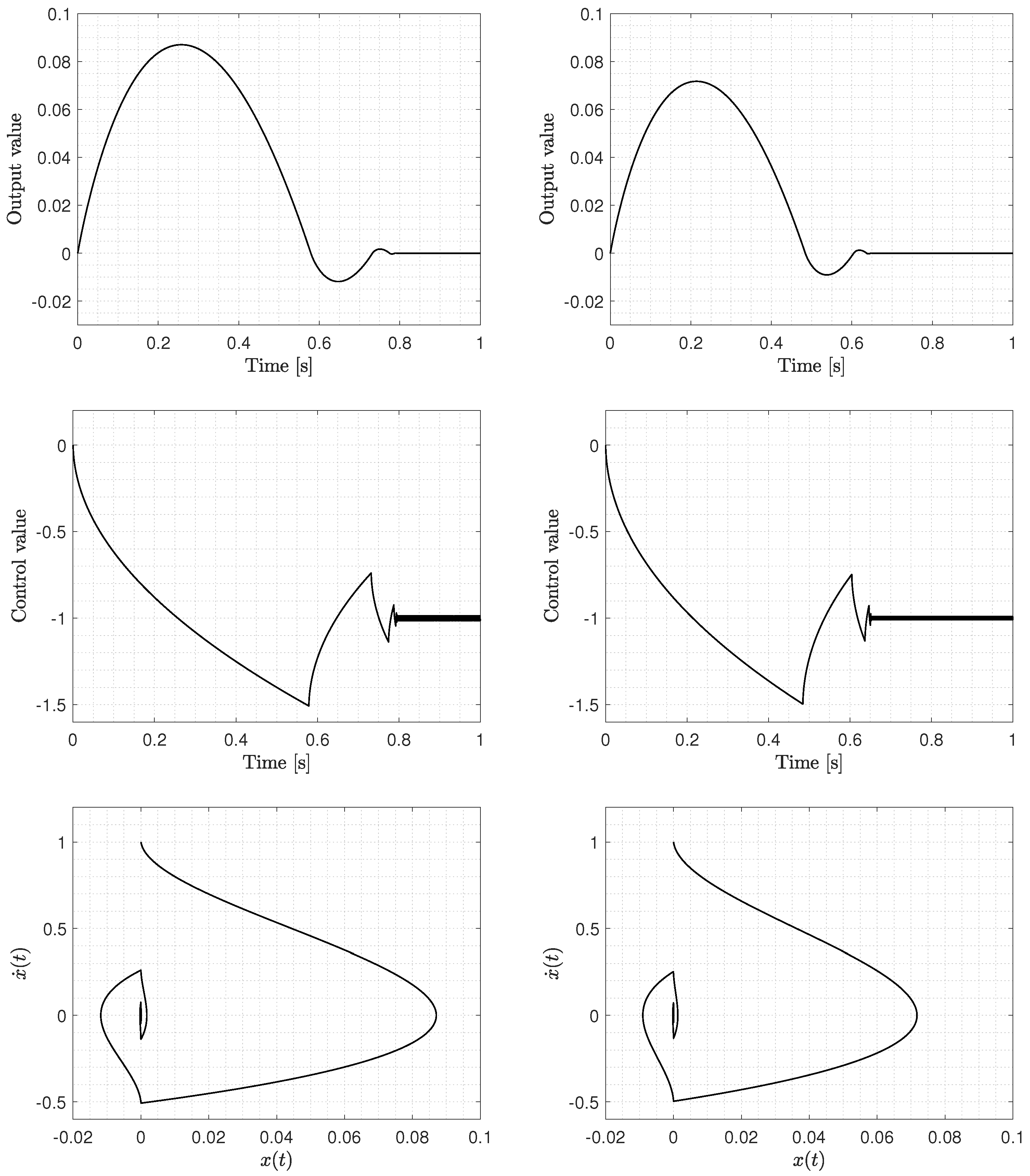
5.1. System without Disturbances

In this case, the feedback gain $\gamma =1$ is considered, as there is no disturbance present in the system. The comparison results of Fractional sliding mode control vs. Mittag–Leffler sliding mode control are shown in Figure 1. It is possible to appreciate that the overshot is somehow lesser in the Mittag–Leffler case than in the fractional one. The control signals are similar and the phase diagram also shows a slightly faster convergence in the case of the Mittag–Leffler controller.

Figure 1. Disturbance free case comparison: Fractional sliding mode control (left column) vs. Mittag–Leffler sliding mode control (right column).

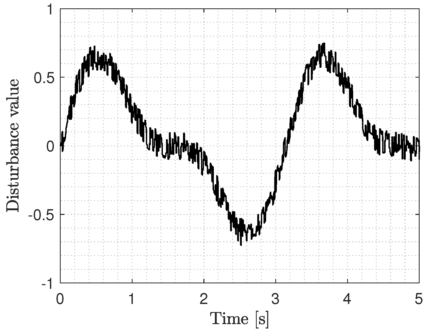
5.2. System with Disturbances

In this case, the feedback gain is set to $\gamma =2.0$ to face system uncertainties. The disturbance is given by

$$d\left(t\right)=0.5sin\left(2t\right)+0.25sin\left(4t\right)+r\left(t\right)$$

(68)

where $r:[0,\infty )\to [-0.1,0.1]$ is a random valued function that updates every 10 ms, see Figure 2. The random pattern is the same for both controllers.

Figure 2. Unknown disturbance.

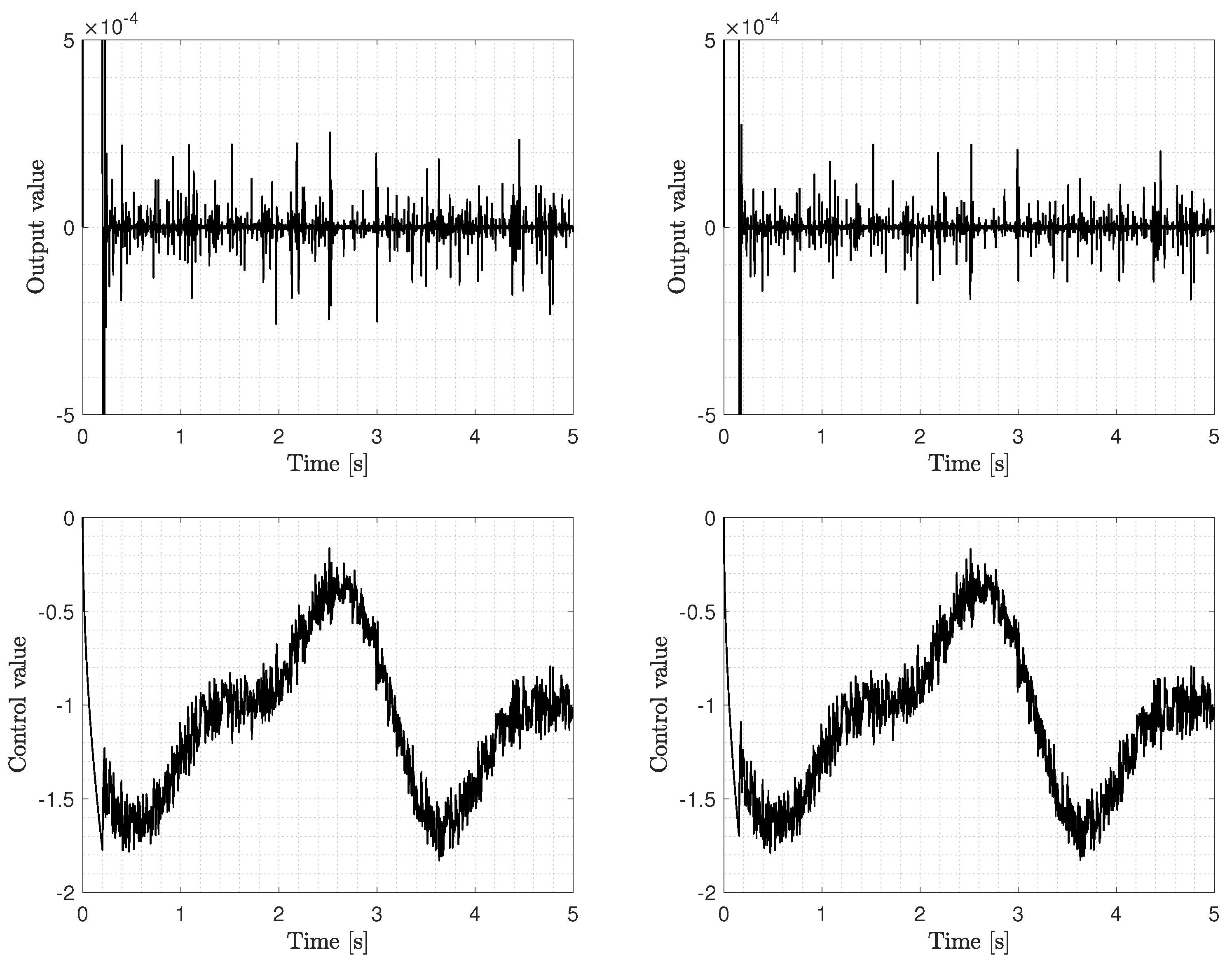
The comparison results are shown in Figure 3. As in the previous case, the output value function is slightly better for the Mittag–Leffler sliding mode controller. Both control signals are similar and reject the disturbance in a good extent.

Figure 3. Disturbed case comparison: Fractional sliding mode control (left column) vs. Mittag–Leffler sliding mode control (right column).

This follows from the known robustness properties of fractional sliding mode controllers.

A more accurate comparison is obtained by relying on the integral square error (ISE) and integral square control (ISC) norms, obtaining the following results for both schemes:

• Fractional sliding mode control:
  ISE $=7.4037\times {10}^{-5}$ and ISC $=6.7932$.
• Mittag–Leffler sliding mode control:
  ISE $=3.3341\times {10}^{-5}$ and ISC $=6.7834$.

This shows that the Mittag–Leffler sliding mode control provides better regulation with less control energy, thus improving the closed-loop performance. It can be mentioned that considering kernels with lower values of $\beta$, the accuracy of the regulation task improves significantly. However, for real-world applications, the order should be kept as high as possible to improve the regularity of the control signal, such that the controller implementation is closer to the theoretical framework, even under the action of moderately fast actuators and conservative computational resources.

6. Discussions

The simulation results show comparable performances as those obtained by implementing well-established control techniques; nonetheless, the contribution of this paper is not limited to a particular class of sliding mode control methodology, rather, it stands for a generalization, and it opens the door to new families of robust control methods. Some limitations of the proposed work are the numerical implementation of the Sonine integral, as it depends on a convolution operation. Nonetheless, the kernel function can be evaluated beforehand to alleviate computational cost, such that the convolution can be approximated by a finite-impulse-response filter. Future research considers some open problems, such as the design of sliding mode controllers with the following kernels: variable-order kernels; Prabhakar functions; Non-Laplace transformable kernels; non-singular kernels; kernels with bounded integrals, etc. Furthermore, the applications of the present methodology in different systems, justifying its implementation in the presence of a large class of non-differentiable disturbances, constitute one of the most interesting avenues of this work for engineering professionals. The potential application cases consider, but are not limited to, the control of unmanned aerial robots, which are subject to gust winds and turbulence effects; robotic manipulators in free-motion with backlash; robots in constrained motion in contact with rough surfaces and diverse tribological phenomena; vehicles immersed in non-Newtonian flows; super-capacitive effects in electric networks; physical and engineering process with noisy measurement; renewable systems (wind and solar energy) subject to non-smooth wind speed and light intensity patterns, etc.

7. Conclusions

The contribution of this paper was proving that a class of singular kernels, even more general than fractional-order, multi-fractional and distributed-order kernels, can be used to propose several different families of uniformly uniformly continuous sliding mode controllers. As mentioned before, the continuous fractional sliding mode control, a powerful and robust methodology, constitutes a very particular case of the larger class of schemes studied in this paper. The present results are of potential interest for a wide range of control applications, where the plant is subject to a general class of disturbances and uncertainties, such as those with multi-fractal indices, or even non-differentiable disturbances that change their regularity over time.