Numerical Solution of Linear Second-Kind Convolution Volterra Integral Equations Using the First-Order Recursive Filters Method

Abstract

A new numerical method for solving Volterra linear convolution integral equations (CVIEs) of the second kind is presented in this work. This new approach uses first-order infinite impulse response digital filters method (IIRFM). Three convolutive kernels were analyzed, the unit kernel and two singular kernels: the logarithmic and generalized Abel kernels. The IIRFM is based on the combined use of the Laplace transformation, a first-order decomposition, and a bilinear transformation. This approach often leads to simple analytical expressions of the approximate solutions, enabling efficient numerical calculation, even using single-precision floating-point numbers. When compared with the method of homotopic perturbations with Laplace transformation (HPM-L), the IIRFM approach does not present, in linear cases, the convergence difficulties inherent to iterative approaches. Unlike most solution methods based on the Laplace transform, the IIRFM has the dual advantage of not requiring the calculation of the Laplace transform of the source function, and of not requiring the systematic calculation of inverse Laplace transforms.

1. Introduction

In the present work, a new method is presented for the numerical solution of the convolutive Volterra integral equations (CVIEs) of the second kind, written in the following form:

$$u_{\lambda ,f}\left(t\right)=f\left(t\right)+\lambda {\int }_0^{t}K(t,t^{\prime })\left\{a_{\mathrm{L}}{u}_{\lambda ,f}\left(t^{\prime }\right)+a_{\mathrm{NL}}\mathrm{NL}\left[u_{\lambda ,f}\left(t^{\prime }\right)\right]\right\}\mathrm{d}{t}^{\prime },$$

(1)

where $K(t,t^{\prime })$ is the kernel of the integral equation; $f\left(t\right)$ is a source function assumed to be continuous; $\lambda ,a_{\mathrm{L}},a_{\mathrm{NL}}\in \mathbb{R}$ are parameters; $\mathrm{NL}\left[u_{\lambda ,f}\left(t\right)\right]$ is a non-linear operator of the desired solution $u_{\lambda ,f}\left(t\right)$. These integral equations are used in a wide variety of scientific areas, such as point mechanics (Abel’s problem), fluid mechanics (water waves scattering, [1]), electrochemistry (voltammetry, [2]), as well as heat transfer (see Section 4).

The linear situation, which is the only one studied in this first paper, corresponds to $a_{\mathrm{NL}}=0$, in which case we find Volterra’s linear integral equations of the second type, defined, for $t⩾0$ and $a_{\mathrm{L}}=1$ [3], by:

$$u_{\lambda ,f}\left(t\right)=f\left(t\right)+\lambda {\int }_0^{t}K(t,t^{\prime })u_{\lambda ,f}\left(t^{\prime }\right)\mathrm{d}{t}^{\prime }.$$

(2)

The present paper studies a particularly important class of Volterra integral equations of the second type, which involves convolutional kernels, depending only upon the difference $t-t^{\prime }$, and written in the general form $K(t,t^{\prime })=K(t-t^{\prime })$. Three kinds of convolution kernels are studied in the present work: the unit kernel $K(t,t^{\prime })=1$; generalized Abel’s kernel $K(t,t^{\prime })=1/{(t-t^{\prime })}^{\alpha }$ with $0<\alpha <1$ and logarithmic kernel $K(t,t^{\prime })=ln\left(\left|t-t^{\prime }\right|\right)$. The last two convolution kernels share the property of being singular at $t=t^{\prime }$.

Note that using the generalized Abel kernel in Volterra’s integral Equation (2) leads to the generalized Abel integral equation of the second kind, as follows:

$$u_{\lambda ,\alpha ,f}\left(t\right)=f\left(t\right)+\lambda {\int }_0^t{\displaystyle \frac{u_{\lambda ,\alpha ,f}\left(t^{\prime }\right)}{{\left(t-t^{\prime }\right)}^{\alpha }}}\mathrm{d}{t}^{\prime }.$$

(3)

A general analytical solution exists in closed form for Abel’s integral equation, involving the calculation (explicit or numerical) of an integral and a series of functions (see [4] (p. 142)):

$$u_{\lambda ,\alpha ,f}\left(t\right)=f\left(t\right)+{\int }_0^{t}R(t–t^{\prime })f\left(t^{\prime }\right)\mathrm{d}{t}^{\prime },\mathrm{with}R\left(t\right)=\sum _{n=1}^{\infty }{\displaystyle \frac{{\left[\lambda \Gamma (1-\alpha )t^{1-\alpha }\right]}^n}{t\Gamma \left[n(1-\alpha )\right]}},$$

(4)

where $\Gamma \left(z\right)={\int }_0^{\infty }{e}^{-x}{x}^{z-1}\mathrm{d}x$ is the Euler gamma function. Result (4) will provide analytical reference solutions for some of the numerical results that will be calculated in this work.

Several approaches based on the Laplace transformation have already been proposed to solve analytically or numerically Volterra (CVIE) or Abel (CAIE) second-kind linear convolution integral equations. In [5,6], the Homotopic Perturbation Method (HPM) and the Laplace transformation were used to numerically determine the solution of various convolution Abel integral equations of the second kind. In [7], systems of coupled convolutive Abel integral equations have been solved numerically using the homotopic analysis method (HAM) introduced by Lio [8,9], coupled with the Laplace transformation. In [10], Bairwa et al. used the q-homotopic analysis and Laplace transformation method (q-HATM) to numerically solve various CAIEs.

All these approaches generally assume that there is an analytical expression for the source function $f\left(t\right)$. There are, however, situations where it is not possible to obtain this expression; for example, when $f\left(t\right)$ is a noisy signal or the result of an experimental measurement. In such cases, the IIR filters method presented here can be very useful for determining the numerical solution of the linear convolution Volterra equations.

The main objective of the present study is therefore to apply the first-order infinite impulse response filters method (IIRFM) proposed by Heyd et al. [11,12] to numerically solve linear Volterra convolutive integral equations of the second kind. The use of infinite impulse response (IIR) digital filters is usually limited to linear time-invariant systems (LTISs), whose dynamics are described by linear ordinary differential equations with constant coefficients, or equivalently by Laplace transfer functions expressed as polynomial fractions. The results presented in this paper make it possible, for the first time, to extend the field of application of IIR filters to linear systems described by Volterra convolutive integral equations of the second kind, which are involved in a wide range of scientific fields, including heat transfer, for example.

This new approach has the great advantage of being non-iterative, which means it has none of the convergence problems inherent in iterative methods. In addition, for some Volterra integral equations, the IIRFM can lead to an analytical expression of the approximate numerical solution, making the calculation very efficient compared with iterative numerical methods.

The results obtained with the IIRFM are compared in this paper with those provided by other numerical approaches, including the homotopic perturbation method with Laplace transformation (HPM-L), the Daubechies wavelet method of Mouley et al. [13], and the polynomial approximation method of Singha et al. [14].

Several new results have been obtained in this work using the IIRFM, such as a very efficient numerical calculation of the function $g_{\lambda }\left(t\right)=1+\mathrm{erf}\left(\lambda \sqrt{\pi t}\right)$ when $\lambda <0$ (see Section 3.2.1) and this even using single-precision floating-point numbers. This new approach to calculating the $\mathrm{erf}\left(\lambda \sqrt{\pi t}\right)$ function could be very usefully incorporated into the free codes currently available, Python, Julia, Octave, and Scilab.

The remainder of this paper is organized as follows. The foundations of the IIRFM and HPM-L methods are outlined in Section 2. The mechanism of the IIRFM is illustrated in Section 3 by numerically solving various linear CVIEs of the second kind. The results obtained by the IIRFM are also compared with those provided by different numerical approaches. Finally, two examples of linear CVIEs used in heat transfers are solved in Section 4 using the IIRFM method.

2. IIRFM and HPM-L Numerical Methods

The two numerical approaches used in this work to solve the integral Equation (2) are outlined in this paragraph, and the main steps involved in their implementation are recalled or introduced here.

2.1. First-Order IIR Filters Method (IIRFM)

The IIRFM consists of numerically solving Equation (2) in discrete time, using sufficiently precise recurrence relations, which are deduced from successive applications of the Laplace transformation, a first-order partial fractions decomposition and of a bilinear transformation.

This method is particularly well suited to solving convolutional linear integral equations (CVIEs), but also ordinary differential equations (ODEs), integro-differential equations (IDEs), and parabolic partial differential equations (PDEs). Each of these differential or integral problems is assumed to be linear and to have constant coefficients.

2.1.1. Principle of the IIRFM Method

The IIRFM consists schematically of replacing each of the differential or integral problems mentioned above, by a set of M independent, first-order, exact, or approximate ordinary differential problems.

Let $(\Sigma )$ be a differential (or integral), linear and invariant problem of the previously mentioned kinds. Let $f\left(t\right)$ be the excitation (or source function) and $u_{\lambda ,f}\left(t\right)$ the response (or solution) of the problem $(\Sigma )$ to the excitation $f\left(t\right)$, for a set of constant $\lambda$ coefficients (see Figure 1).

Figure 1. Differential or integral, linear, and invariant problems. (a) Schematic representation in direct space. (b) Schematic representation in Laplace space.

Let us symbolically denote $F(\int u_{\lambda ,f},u_{\lambda ,f},{\dot{u}}_{\lambda ,f},f,\lambda ,t)=0$ the equation that governs the dynamics of $(\Sigma )$ in direct space (see Figure 1a). To simplify the presentation, we assume at this stage that the initial condition on $u_{\lambda ,f}\left(t\right)$ is null: $u_{\lambda ,f}\left(0\right)=0$. Since the functional relationship $F=0$ is linear and has constant coefficients, the Laplace transformation $\mathcal{L}$ can be applied to it. This gives the algebraic relationship ${\overline{u}}_{\lambda ,f}\left(s\right)=H\left(s\right)\overline{f}\left(s\right)$, which governs the dynamics of $(\Sigma )$ in the Laplace space, where $H\left(s\right)$ is the Laplace transfer function of the system (see Figure 1b), with ${\overline{u}}_{\lambda ,f}\left(s\right)=\mathcal{L}\left[u_{\lambda ,t}\left(t\right)\right]$ and $\overline{f}\left(s\right)=\mathcal{L}\left[f\left(t\right)\right]$.

To transform the equation $F(\int u_{\lambda ,f},u_{\lambda ,f},{\dot{u}}_{\lambda ,f},f,\lambda ,t)=0$ into M independent, linear, first-order ODEs with constant coefficients, the function $H\left(s\right)-C_0$, with $C_0$ as a constant, is first approximated by a rational fraction ${\mathrm{RF}}^M\left(s\right)$ of the following form:

$${\mathrm{RF}}^M\left(s\right)={\displaystyle \frac{{\sum }_{n=0}^{M-1}{h}_n\left(\lambda \right)s^n}{{\sum }_{m=0}^M{\ell }_m\left(\lambda \right)s^m}},$$

(5)

where $\{h_n,{\ell }_m\}$ is a set of $2M+1$ constant real coefficients, determined by interpolation (by least squares or Chebyshev for example) or approximation (of Padé for example) of the $H\left(s\right)-C_0$ function. Note that the value of the constant $C_0$ depends on the problem under consideration. In the case of linear convolutional Volterra integral equations of the second kind (CVIE), which will be examined in detail later in this work, the value $C_0=1$ is chosen.

The rational fraction ${\mathrm{RF}}^M\left(s\right)$ is then decomposed, by partial fractions decomposition, in the usual form, as follows:

$$\begin{array}{cc}\hfill {\mathrm{RF}}^M\left(s\right)& =\sum _{i=1}^{N_1}{\displaystyle \frac{r_i}{s-p_i}}+\sum _{j=1}^{N_2}{\displaystyle \frac{c_j+d_{j}s}{e_j+f_{j}s+g_j{s}^2}},\hfill \\ \hfill & =\sum _{i=1}^{N_1}{H}_i^1\left(s\right)+\sum _{j=1}^{N_2}{H}_j^2\left(s\right),\hfill \end{array}$$

(6)

where $N_1+2N_2=M$ and $c_j$, $d_j$, $e_j$, $f_j$, $g_j$, $r_i$, $p_i$ are real constants. Note that it is assumed here that the multiplicity ${\nu }_i$ of each pole $p_i$ is unity. This property is usually guaranteed by the fact that the poles are approximated and are calculated numerically here. Finally, each second-order transfer function $H_j^2$ is decomposed into single complex elements, in the following form:

$$H_j^2\left(s\right)={\displaystyle \frac{{\alpha }_j+\mathrm{i}{\beta }_j}{s-{\underline{z}}_j}}+{\displaystyle \frac{{\alpha }_j-\mathrm{i}{\beta }_j}{s-{\underline{z}}_j^{*}}},$$

(7)

where ${\underline{z}}_j=x_j+\mathrm{i}{y}_j$ and ${\underline{z}}_j^{*}=x_j-\mathrm{i}{y}_j$ are the complex conjugate roots (with $y_j\ne 0$) of the polynomial equation $e_j+f_{j}s+g_j{s}^2=0$. The real constants ${\alpha }_j$ and ${\beta }_j$ are ${\alpha }_j=d_j/2$ and ${\beta }_j=-{\displaystyle \frac{1}{2}}(c_j+d_j{x}_j)/y_j$, respectively. The previous results can be combined by writing ${\mathrm{RF}}^M\left(s\right)$ as a combination of M first-order transfer functions with complex coefficients, as follows:

$${\mathrm{RF}}^M\left(s\right)=\sum _{i=1}^M{\displaystyle \frac{a_{M,i}\left(\lambda \right)}{b_{M,i}\left(\lambda \right)+s}},$$

(8)

where $a_{M,i}\left(\lambda \right),b_{M,i}\left(\lambda \right)\in \mathbb{Z}$. Finally, the exact $H\left(s\right)$ transfer function of the system is replaced by a transfer function $H^M\left(s\right)$ written in the following form:

$$H^M\left(s\right)=C_0+\sum _{i=1}^M{\displaystyle \frac{a_{M,i}\left(\lambda \right)}{b_{M,i}\left(\lambda \right)+s}}.$$

(9)

This is a founding result of the IIRFM. Note that in certain situations, the transfer function $H^M\left(s\right)$ may coincide with the exact transfer function (see for example Section 3.1).

Using result (9), the approximate solution ${\overline{u}}_{\lambda ,f}^{\mathrm{IIR},M}\left(s\right)$ can be expressed in the Laplace space as

$${\overline{u}}_{\lambda ,f}^{\mathrm{IIR},M}\left(s\right)=H^M\left(s\right)\overline{f}\left(s\right)=C_0\overline{f}\left(s\right)+\sum _{i=1}^M{\displaystyle \frac{a_{M,i}\left(\lambda \right)}{b_{M,i}\left(\lambda \right)+s}}\overline{f}\left(s\right),$$

(10)

which can also be written as ${\overline{u}}_{\lambda ,f}^{\mathrm{IIR},M}\left(s\right)={\overline{u}}_{\lambda ,f,0}^{\mathrm{IIR},M}\left(s\right)+{\sum }_{i=1}^M{\overline{u}}_{\lambda ,f,i>0}^{\mathrm{IIR},M}\left(s\right)$, with

$${\overline{u}}_{\lambda ,f,0}^{\mathrm{IIR},M}\left(s\right)=C_0\overline{f}\left(s\right)\mathrm{and}{\overline{u}}_{\lambda ,f,i>0}^{\mathrm{IIR},M}\left(s\right)={\displaystyle \frac{a_{M,i}\left(\lambda \right)}{b_{M,i}\left(\lambda \right)+s}}\overline{f}\left(s\right),$$

(11)

which are the approximate partial solutions of the problem in the Laplace space.

The approximate solution $u_{\lambda ,f}^{\mathrm{IIR},M}\left(t\right)$ of the problem in the direct space remains to be determined. Several approaches are possible (without being exhaustive):

• It is possible to consider that each first-order partial transfer function $a_{M,i}\left(\lambda \right)/[b_{M,i}\left(\lambda \right)\hspace{0.17em}+s]$ corresponds to the Laplace transform of a first-order linear ODE with constant coefficients and zero initial condition, for $i=1,2,\cdots ,M$:

  $${\displaystyle \frac{a_{M,i}\left(\lambda \right)}{b_{M,i}\left(\lambda \right)+s}}={\displaystyle \frac{{\overline{u}}_{\lambda ,f,i>0}^{\mathrm{IIR},M}\left(s\right)}{\overline{f}\left(s\right)}}\iff {\dot{u}}_{\lambda ,f,i>0}^{\mathrm{IIR},M}\left(t\right)+b_{M,i}\left(\lambda \right)u_{\lambda ,f,i>0}^{\mathrm{IIR},M}\left(t\right)=a_{M,i}\left(\lambda \right)f\left(t\right),$$

  (12)

  where $u_{\lambda ,f,i>0}^{\mathrm{IIR},M}\left(0\right)=0$. The partial solutions $u_{\lambda ,f,i>0}^{\mathrm{IIR},M}\left(t\right)$ are obtained by applying the method of variation of constants, giving

  $$u_{\lambda ,f}^{\mathrm{IIR},M}\left(t\right)=C_{0}f\left(t\right)+\sum _{i=1}^M{a}_{M,i}\left(\lambda \right){\int }_0^{t}f\left(t^{\prime }\right)e^{-\left[b_{M,i}\left(\lambda \right)(t-t^{\prime })\right]}\mathrm{d}{t}^{\prime }.$$

  (13)
  Depending on the expression of $f\left(t\right)$, the M convolutional integrals figuring in (13) will be calculated analytically or numerically.
• Noting that ${\mathcal{L}}^{-1}\left[{\displaystyle \frac{a_{M,i}\left(\lambda \right)}{b_{M,i}\left(\lambda \right)+s}}\right]=a_{M,i}\left(\lambda \right)e^{-b_{M,i}\left(\lambda \right)t}$, the result (13) can be found directly by applying the convolution theorem.
• Finally, it is also possible to transform ordinary differential Equation (12) into partial recurrence relations by applying a bilinear transformation $s\to {\displaystyle \frac{2}{T_e}}{\displaystyle \frac{z-1}{z+1}}$[12] to each partial transfer function $a_{M,i}\left(\lambda \right)/[b_{M,i}\left(\lambda \right)+s]$. It follows that the partial solution $u_{\lambda ,f,i>0}^{\mathrm{IIR},M}\left(t_k\right)$ verifies the following recurrence relation for $t_k=k{T}_e$, $k⩾1$, $i=1,\cdots ,M$ and $u_{\lambda ,f,i>0}^{\mathrm{IIR},M}\left(t_0\right)=0$:

  $$\left|\begin{array}{c}{u}_{\lambda ,f,0}^{\mathrm{IIR},M}\left(t_k\right)=C_{0}f\left(t_k\right)\mathrm{and}{u}_{\lambda ,f,0}^{\mathrm{IIR},M}\left(t_0\right)=0,\hfill \\ \\ u_{\lambda ,f,i>0}^{\mathrm{IIR},M}\left(t_k\right)={\displaystyle \frac{2-T_e{b}_{M,i}\left(\lambda \right)}{2+T_e{b}_{M,i}\left(\lambda \right)}}{u}_{\lambda ,f,i>0}^{\mathrm{IIR},M}\left(t_{k-1}\right)+{\displaystyle \frac{a_{M,i}\left(\lambda \right)}{2+T_e{b}_{M,i}\left(\lambda \right)}}\left[f\left(t_k\right)+f\left(t_{k-1}\right)\right],\hfill \end{array}\right.$$

  (14)

  where $T_e>0$ is the calculation step.

This latter approach will be discussed in detail in the remainder of this paper, which focuses on the numerical solution of linear convolutional Volterra integral equations of the second type (CVIE), for which it is recalled that $C_0=1$.

2.1.2. Application of the IIRFM to the Case of Second-Kind CVIEs

The different steps of the IIRFM are schematically as follows:

Step 1.

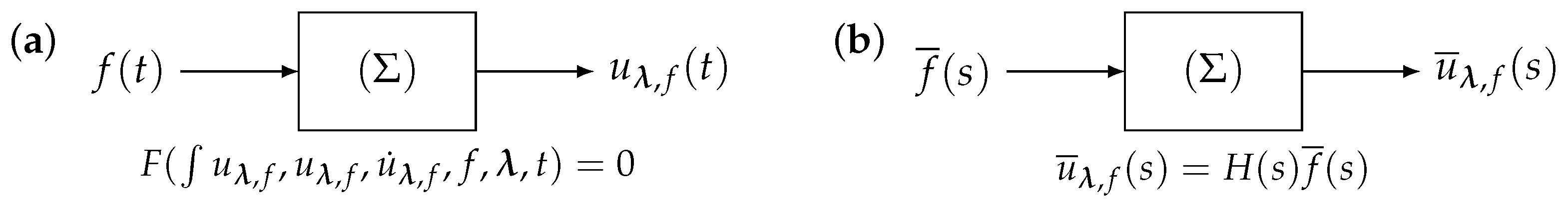
The Laplace transformation ($\mathcal{L}$) is applied to Equation (1):

$$\mathcal{L}\left[\left(1\right)\right]\Rightarrow {\overline{u}}_{\lambda ,f}\left(s\right)=\overline{f}\left(s\right)+\lambda \mathcal{L}\left[{\int }_0^{t}K(t-t^{\prime })\left\{a_{\mathrm{L}}{u}_{\lambda ,f}\left(t^{\prime }\right)+a_{\mathrm{NL}}\mathrm{NL}\left[u_{\lambda ,f}\left(t^{\prime }\right)\right]\right\}\mathrm{d}{t}^{\prime }\right],$$

(15)

with ${\overline{u}}_{\lambda ,f}\left(s\right)=\mathcal{L}\left[u_{\lambda ,f}\left(t\right)\right]$ and $\overline{f}\left(s\right)=\mathcal{L}\left[f\left(t\right)\right]$. Using the convolution theorem, the Laplace transform of the previous integral can be written as follows:

$$\begin{array}{cc}\hfill & \mathcal{L}\left[{\int }_0^{t}K(t-t^{\prime })\left\{a_{\mathrm{L}}{u}_{\lambda ,f}\left(t^{\prime }\right)+a_{\mathrm{NL}}\mathrm{NL}\left[u_{\lambda ,f}\left(t^{\prime }\right)\right]\right\}\mathrm{d}{t}^{\prime }\right]\hfill \\ \hfill & =\overline{K}\left(s\right)\times \left\{a_{\mathrm{L}}{\overline{u}}_{\lambda ,f}\left(s\right)+a_{\mathrm{NL}}\overline{\mathrm{NL}}\left[u_{\lambda ,f}\right]\left(s\right)\right\},\hfill \end{array}$$

(16)

where $\overline{K}\left(s\right)=\mathcal{L}\left[K(t,0)\right]$ and $\overline{\mathrm{NL}}\left[u_{\lambda ,f}\right]\left(s\right)=\mathcal{L}\left\{\mathrm{NL}\left[u_{\lambda ,f}\left(t\right)\right]\right\}$, of which the analytical expression is usually unknown.

This gives the following expression for ${\overline{u}}_{\lambda ,f}\left(s\right)$:

$${\overline{u}}_{\lambda ,f}\left(s\right)={\displaystyle \frac{1}{1-\lambda a_{\mathrm{L}}\overline{K}\left(s\right)}}\overline{f}\left(s\right)+{\displaystyle \frac{\lambda a_{\mathrm{NL}}\overline{K}\left(s\right)}{1-\lambda a_{\mathrm{L}}\overline{K}\left(s\right)}}\overline{\mathrm{NL}}\left[u_{\lambda ,f}\right]\left(s\right).$$

(17)

Let us write $H_{\mathrm{L}}(s,\lambda )=1/(1-\lambda a_{\mathrm{L}}\overline{K}\left(s\right))$ and $H_{\mathrm{NL}}(s,\lambda )=\lambda a_{\mathrm{NL}}\overline{K}\left(s\right)/(1-\lambda a_{\mathrm{L}}\overline{K}\left(s\right))$. Three of the following situations are possible:

(a)

$a_{\mathrm{NL}}=0$ and $a_{\mathrm{L}}=1$: this is the linear situation, for which the Volterra problem of the second kind can be described as a linear dynamics system with Laplace transfer function $H_{\mathrm{L}}(s,\lambda )={\overline{u}}_{\lambda ,f}\left(s\right)/\overline{f}\left(s\right)=1/(1-\lambda \overline{K}\left(s\right))$.

With the exception of the special case of the unit kernel $K(t,t^{\prime })=1$, note that the transfer function $H_{\mathrm{L}}(s,\lambda )$ does not have the usual form of a quotient of polynomials in s, as it is usually the case for LTIS. Several examples of linear situations are presented in Section 3.

(b)

$a_{\mathrm{NL}}=1$ and $a_{\mathrm{L}}=0$: the result is a purely non-linear situation. To solve the problem numerically, the expression of the Laplace transform $\overline{\mathrm{NL}}\left[u_{\lambda ,f}\right]\left(s\right)$ must be specified. Various approaches can be considered for this purpose, such as the Adomian polynomials method [15,16].

(c)

$a_{\mathrm{NL}}\ne 0$ and $a_{\mathrm{L}}\ne 0$: this is a hybrid situation, in which the IIRFM numerical solution uses both the Laplace transfer function and the Adomian polynomials approach.

We now explain the next steps of the IIRFM, but only in the case of the linear situation ($a_{\mathrm{NL}}=0$ and $a_{\mathrm{L}}=1$).

Step 2.

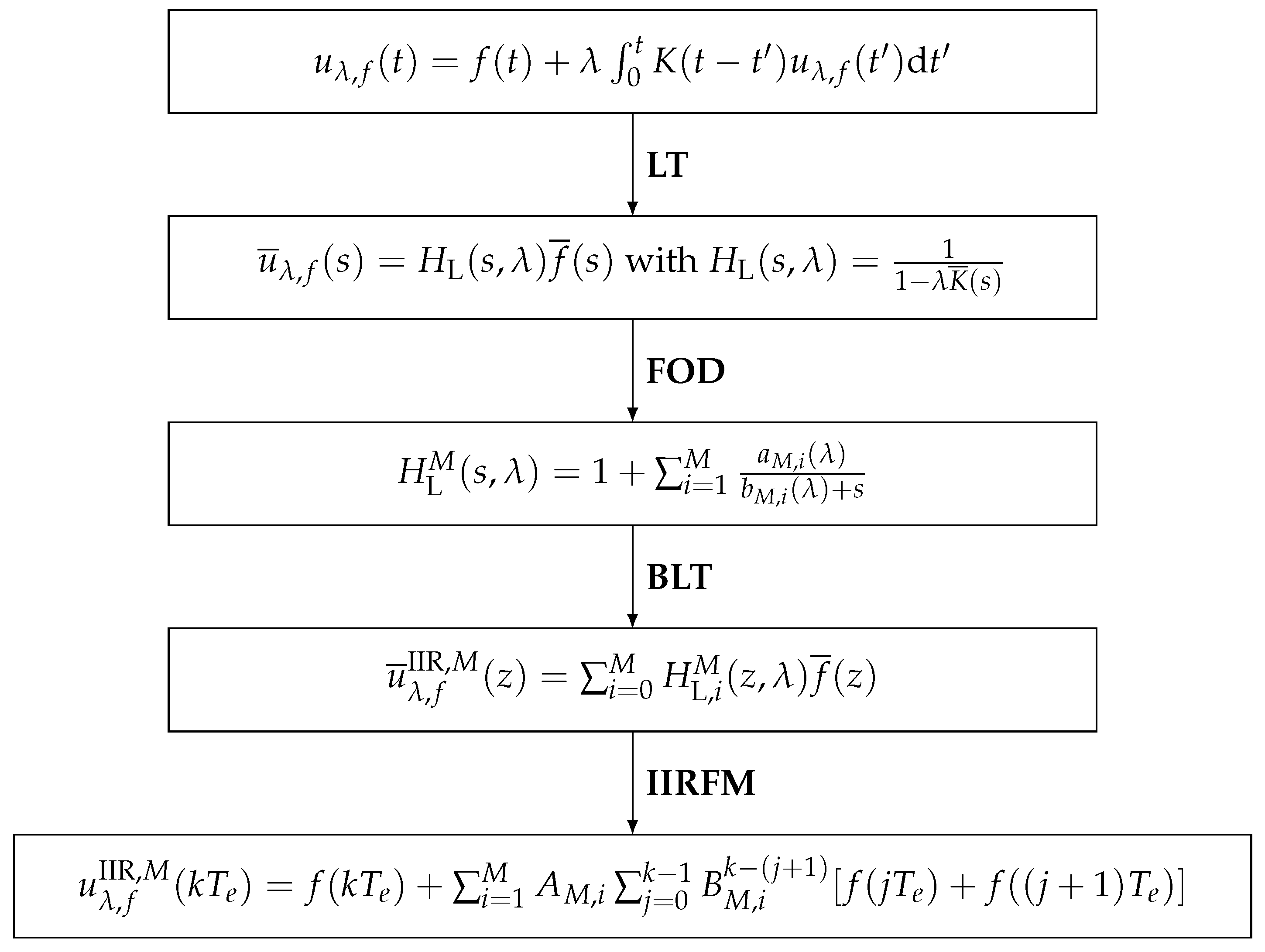
To solve the linear Volterra problem using the transfer function $H_{\mathrm{L}}(s,\lambda )$, it is first rewritten as a linear combination of $M+1$ first-order transfer functions (first-order partial fractions decomposition, noted FOD):

$$H_{\mathrm{L}}^M(s,\lambda )=1+\sum _{i=1}^M{\displaystyle \frac{a_{M,i}\left(\lambda \right)}{b_{M,i}\left(\lambda \right)+s}},$$

(18)

with $a_{M,i},b_{M,i}\in \mathbb{Z}$. This particular expression (other expressions are possible) of the transfer function $H_{\mathrm{L}}(s,\lambda )$ is the founding point of the IIRFM applied to second-kind CVIEs. By introducing $M+1$ partial transfer functions $H_{\mathrm{L},i}^M(s,\lambda )$, we can rewrite Equation (18) as $H_{\mathrm{L}}^M(s,\lambda )={\sum }_{i=0}^M{H}_{\mathrm{L},i}^M(s,\lambda )$ with $H_{\mathrm{L},0}^M(s,\lambda )=1$. With these notations, ${\overline{u}}_{\lambda ,f}\left(s\right)$ can still be written as:

$${\overline{u}}_{\lambda ,f}\left(s\right)=\sum _{i=0}^M{H}_{\mathrm{L},i}^M(s,\lambda )\overline{f}\left(s\right)=\sum _{i=0}^M{\overline{u}}_{\lambda ,f,i}\left(s\right).$$

(19)

Depending on the convolution kernel considered, Equation (18) can be an exact form (see Section 3.1) or an approximation of $H_{\mathrm{L}}(s,\lambda )$ (see Section 3.2, Section 3.3 and Section 4). In the latter case, coefficients $a_{M,i}$ and $b_{M,i}$ are determined by rational interpolation of the function $G(s,\lambda )=H_{\mathrm{L}}(s,\lambda )-1$. We will come back to this point later.

The choice of (18) ensures that the approximate form $H_{\mathrm{L}}^M(s,\lambda )$ tends to be 1 for $s\to \infty$, as does the exact form $H_{\mathrm{L}}(s,\lambda )$ for the convolution kernels considered in this study, unit, generalized Abel, and logarithmic. This also reduces the interpolation interval to a set of s values close to 0, as will be shown later.

The solution obtained by the IIRFM is now denoted by $u_{\lambda ,f}^{\mathrm{IIR},M}\left(t\right)$.

Step 3.

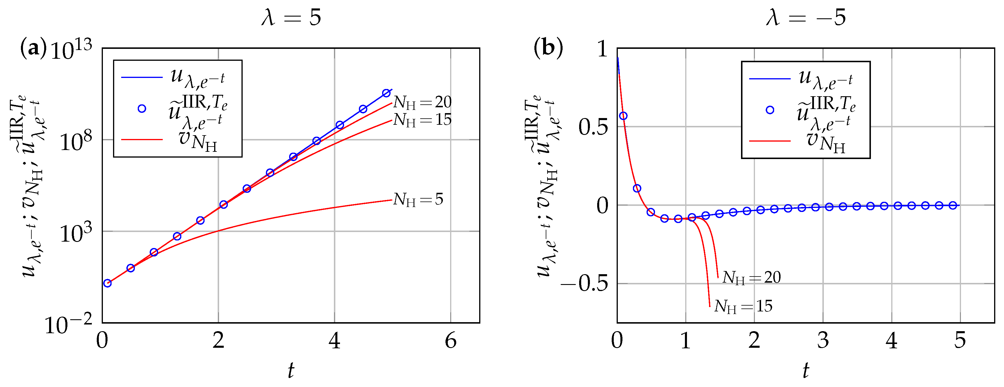
A bilinear transformation $s\to {\displaystyle \frac{2}{T_e}}{\displaystyle \frac{z-1}{z+1}}$ ([12]) is applied to the transfer function $H_{\mathrm{L}}^M(s,\lambda )$, where $T_e\in {\mathbb{R}}^{+}$ is a uniform time step (or sampling period) and z is the complex number introduced in the definition of the z-transform (noted here $\mathcal{Z}$) of a discrete-time signal $x\left(k{T}_e\right)$: $\mathcal{Z}\left[x\left(k{T}_e\right)\right]=\overline{x}\left(z\right)={\sum }_{k=0}^{\infty }x\left(k{T}_e\right)z^{-k}$, with $k\in \mathbb{N}$. After a few algebraic manipulations, we obtain the following z transfer function:

$$H_{\mathrm{L}}^M(z,\lambda )=1+\sum _{i=1}^M{\displaystyle \frac{A_{M,i}+A_{M,i}{z}^{-1}}{1-B_{M,i}{z}^{-1}}}=\sum _{i=0}^M{H}_{\mathrm{L},i}^M(z,\lambda ),$$

(20)

with $H_{\mathrm{L},0}^M(z,\lambda )=1$, $H_{\mathrm{L},i>0}^M(z,\lambda )=(A_{M,i}+A_{M,i}{z}^{-1})/(1-B_{M,i}{z}^{-1})$, $A_{M,i}=a_{M,i}{T}_e/(2+b_{M,i}{T}_e)$, $B_{M,i}=(2-b_{M,i}{T}_e)/(2+b_{M,i}{T}_e)$ and $b_{M,i}{T}_e\ne -2$.

The z-transform ${\overline{u}}_{\lambda ,f}^{\mathrm{IIR},M}\left(z\right)$ obtained by the IIRFM satisfies the following relations:

$${\overline{u}}_{\lambda ,f}^{\mathrm{IIR},M}\left(z\right)=H_{\mathrm{L}}^M(z,\lambda )\overline{f}\left(z\right)=\sum _{i=0}^M{H}_{\mathrm{L},i}^M(z,\lambda )\overline{f}\left(z\right),$$

(21)

where $\overline{f}\left(z\right)=\mathcal{Z}\left[f\left(k{T}_e\right)\right]$ is the z-transform of the source function $f\left(t\right)$. The solution ${\overline{u}}_{\lambda ,f}^{\mathrm{IIR},M}\left(z\right)$ can be further decomposed into a sum of $M+1$ partial solutions, as follows: ${\overline{u}}_{\lambda ,f}^{\mathrm{IIR},M}\left(z\right)={\sum }_{i=0}^M{\overline{u}}_{\lambda ,f,i}^{\mathrm{IIR},M}\left(z\right)$ with ${\overline{u}}_{\lambda ,f,i}^{\mathrm{IIR},M}\left(z\right)=H_{\mathrm{L},i}^M(z,\lambda )\overline{f}\left(z\right)$.

Step 4.

The solution is calculated in the discrete time space using recurrence relations deduced from transfer function (20). In order not to unnecessarily complicate the theoretical developments in this paragraph, it is assumed here that the function $f\left(t\right)$ is zero at the initial instant, which also imposes a zero initial condition for the solution: $u_{\lambda ,f}\left(0\right)=0$. The case of a non-zero initial condition will be considered later in this work (see Section “Exponential Source Term $f\left(t\right)=e^{-t}$”). The discrete-time solution at time $t_k=k{T}_e$ is denoted by $u_{\lambda ,f}^{\mathrm{IIR},M}\left(k{T}_e\right)={\sum }_{i=0}^M{u}_{\lambda ,f,i}^{\mathrm{IIR},M}\left(k{T}_e\right)$.

Using time-shifting properties $\mathcal{Z}\left[x\left((k-m)T_e\right)\right]=z^{-m}\mathcal{Z}\left[x\left(k{T}_e\right)\right]$ and linearity $\mathcal{Z}\left[a_{m}x\left(k{T}_e\right)\right]=a_m\mathcal{Z}\left[x\left(k{T}_e\right)\right]$ of the z-transform, the following $M+1$ partial recurrence relations are obtained:

$$\left|\begin{array}{c}{u}_{\lambda ,f,0}^{\mathrm{IIR},M}\left(k{T}_e\right)=f\left(k{T}_e\right)\forall k>0\mathrm{and}{u}_{\lambda ,f,0}^{\mathrm{IIR},M}\left(0\right)=0,\hfill \\ u_{\lambda ,f,i\ne 0}^{\mathrm{IIR},M}\left(k{T}_e\right)=B_{M,i}{u}_{\lambda ,f,i\ne 0}^{\mathrm{IIR},M}\left((k-1)T_e\right)+A_{M,i}\left[f\left(k{T}_e\right)+f\left((k-1)T_e\right)\right],\forall k⩾1,\hfill \\ \mathrm{with}{u}_{\lambda ,f,i\ne 0}^{\mathrm{IIR},M}\left(0\right)=0.\hfill \end{array}\right.$$

(22)

Note that the second recurrence relation of (22) leads to the following explicit expression for the partial solution $u_{\lambda ,f,i\ne 0}^{\mathrm{IIR},M}\left(k{T}_e\right)$:

$$u_{\lambda ,f,i\ne 0}^{\mathrm{IIR},M}\left(k{T}_e\right)=A_{M,i}\sum _{j=0}^{k-1}{B}_{M,i}^{k-(j+1)}\left[f\left(j{T}_e\right)+f\left((j+1)T_e\right)\right].$$

(23)

This is a particularly important result of this study. Depending on the expression of the source term $f\left(t\right)$, the expression of Equation (23) can be further simplified, as will be seen with some of the examples to be studied in Section 3.

The complete solution $u_{\lambda ,f}^{\mathrm{IIR},M}\left(k{T}_e\right)$ provided at time $t_k=k{T}_e$ by the IIRFM is therefore of the following general form:

$$u_{\lambda ,f}^{\mathrm{IIR},M}\left(k{T}_e\right)=f\left(k{T}_e\right)+\sum _{i=1}^M{A}_{M,i}\sum _{j=0}^{k-1}{B}_{M,i}^{k-(j+1)}\left[f\left(j{T}_e\right)+f\left((j+1)T_e\right)\right].$$

(24)

In the most general case, the calculation of $u_{\lambda ,f}^{\mathrm{IIR},M}\left(k{T}_e\right)$ involves two sums, with a total of $M\times k$ terms. As a result, calculation times can become significant as k increases. However, these calculation times can be significantly reduced when an explicit expression ${\Xi }_{M,i}\left(k,T_e,B_{M,i},f\right)$ of ${\sum }_{j=0}^{k-1}{B}_{M,i}^{k-(j+1)}\left[f\left(j{T}_e\right)+f\left((j+1)T_e\right)\right]$ exists. In this case, the numerical solution $u_{\lambda ,f}^{\mathrm{IIR},M}\left(k{T}_e\right)$ can be written as

$$u_{\lambda ,f}^{\mathrm{IIR},M}\left(k{T}_e\right)=f\left(k{T}_e\right)+\sum _{i=1}^M{A}_{M,i}{\Xi }_{M,i}\left(k,T_e,B_{M,i},f\right),$$

(25)

and then the calculation only involves a single sum of M terms, which significantly reduces computation times.

Equations (24) and (25) are the key results of the IIRFM applied to the numerical solution of linear CVIEs of the second kind. In contrast to the method of homotopic perturbations with Laplace transformation (HPM-L), which will be presented in the following paragraph, it is not necessary with the IIRFM to calculate the Laplace transform $\overline{f}\left(s\right)$ of the source function $f\left(t\right)$ in order to numerically solve the problem under consideration. This is a considerable advantage of the IIRFM, as there are situations where the calculation of $\overline{f}\left(s\right)$ is not possible. This is the case, for example, if $f\left(t\right)$ includes a random component (like noise) or is the result of experimental measurements.

The block diagram shown in Figure 2 summarizes the main steps of the IIRFM as applied to the numerical solution of linear CVIEs of the second kind.

Figure 2. Main steps of the IIRFM, as applied to the numerical solution of linear CVIEs ($a_{\mathrm{L}}=1$ and $a_{\mathrm{NL}}=0$) of the second kind, with LT: Laplace transform; FOD: first-order partial fractions decomposition; BLT: bilinear transformation; IIRFM: final result of the IIRFM method.

2.2. Homotopic Peturbation Method with Laplace Transform (HPM-L)

In what follows, some of the results obtained by the IIRFM will be compared, among others, with the results provided by the homotopic perturbation method with Laplace transformation (HPM-L), an approach that also relies on an initial application of the Laplace transformation to Equation (2). We therefore recall the main results that define this method in the linear case only ($a_{\mathrm{NL}}=0$ and $a_{\mathrm{L}}=1$).

The homotopic perturbation method (HPM) was introduced by He [17,18,19] to solve ordinary differential equations (ODEs) or partial differential equations (PDEs), whether linear or non-linear. This method can also be applied to the case of linear CVIEs of type (2) and to ordinary integro-differential equations. In the present case, the HPM approach consists first of constructing a homotopy $\mathcal{H}(v,p)$ associated with Equation (2), where $p\in [0,1]$ is an embedded parameter and v is an approximate solution to Equation (2). The homotopy is constructed in such a way that at the limit where $p\to 1$, the solution v of the homotopic equation $\mathcal{H}(v,p)=0$ converges to the solution u of the problem under consideration. The method of homotopic perturbations with Laplace transform (HPM-L) used in this work consists of using the Laplace integral transformation $\mathcal{L}$ in the homotopy construction process. It is possible to construct $\mathcal{H}(v,p)$ directly from the Laplace transform of a differential Equation [20], which is generally well suited to the case of non-steady PDEs. In the case of EDOs and CVIEs, it is generally preferable to rewrite the equations using the direct $\mathcal{L}$ and inverse ${\mathcal{L}}^{-1}$ Laplace transformations [21,22]:

$$\mathcal{L}\Rightarrow \mathcal{L}\left[u_{\lambda ,f}\left(t\right)\right]=\mathcal{L}\left[f\left(t\right)\right]+\lambda \mathcal{L}\left[K(t,0)\right]\times \mathcal{L}\left[u_{\lambda ,f}\left(t\right)\right].$$

(26)

By noting $\mathcal{L}\left[K(t,0)\right]=\overline{K}\left(s\right)$, the Laplace transform of (2) can be written in the following form:

$$\mathcal{L}\left[u_{\lambda ,f}\left(t\right)\right]=\mathcal{L}\left[f\left(t\right)\right]+\lambda \overline{K}\left(s\right)\times \mathcal{L}\left[u_{\lambda ,f}\left(t\right)\right].$$

(27)

It remains to apply the inverse Laplace transformation ${\mathcal{L}}^{-1}$ to algebraic Equation (27), which leads to the following statement for $u_{\lambda ,f}\left(t\right)$:

$$u_{\lambda ,f}\left(t\right)=f\left(t\right)+\lambda {\mathcal{L}}^{-1}\left\{\overline{K}\left(s\right)\times \mathcal{L}\left[u_{\lambda ,f}\left(t\right)\right]\right\}.$$

(28)

Finally, from (28) the following $\mathcal{H}(v,p)$ homotopy can be constructed:

$$\mathcal{H}(v,p)=v\left(t\right)-f\left(t\right)-p\lambda {\mathcal{L}}^{-1}\left\{\overline{K}\left(s\right)\times \mathcal{L}\left[v\left(t\right)\right]\right\},$$

(29)

which verifies the following relations:

$$\left|\begin{array}{c}\mathcal{H}(v,0)=0\Rightarrow v\left(t\right)=f\left(t\right),\hfill \\ \mathcal{H}(v,1)=0\Rightarrow v\left(t\right)=f\left(t\right)+\lambda {\mathcal{L}}^{-1}\left\{\overline{K}\left(s\right)\times \mathcal{L}\left[v\left(t\right)\right]\right\}.\hfill \end{array}\right.$$

(30)

The second equation in (30) shows that the solution to the homotopic equation $\mathcal{H}(v,1)=0$ is indeed the solution to the initial problem (2). To solve this homotopic equation, the perturbation method is generally used, which consists of writing the solution $v_H(t,p)$ of (29) as a series expansion of the embedded parameter p, as follows:

$$v_H(t,p)=\sum _{n=0}^{\infty }{p}^n{v}_n\left(t\right).$$

(31)

Assuming that series (31) is convergent, we then have the following result:

$$v\left(t\right)=\underset{p\to 1}{lim}{v}_H(t,p)=v_0\left(t\right)+v_1\left(t\right)+\cdots +v_n\left(t\right)+\cdots .$$

(32)

Two situations can be encountered:

• ${lim}_{p\to 1}{v}_H(t,p)$ converges to a closed form, in which case the homotopic perturbation method leads to an analytic solution of Equation (2);
• There is no known closed form of ${lim}_{p\to 1}{v}_H(t,p)$, in which case the series is generally truncated at the $N_{\mathrm{H}}+1$ first terms and the solution of the problem is written in the following approximate form:

  $$v_{N_{\mathrm{H}}}\left(t\right)=\sum _{n=0}^{N_{\mathrm{H}}}{v}_n\left(t\right).$$

  (33)

It is the last situation that is of particular interest in the present work, because even if series (32) is convergent, the value of the parameter $\lambda$ can considerably influence the speed of convergence of $v_{N_{\mathrm{H}}}\left(t\right)$. Situations may therefore arise where the number $N_{\mathrm{H}}+1$ of terms to be considered may become numerically prohibitive, making the HPM-L method imprecise, inoperative, or very difficult to implement.

The $v_n\left(t\right)$ functions are obtained by incorporating Equation (31) into the homotopic equation $\mathcal{H}(v,p)=0$. Using the linearity of the Laplace transformation, the following recurrence relation of the given problem is obtained as follows:

$$\sum _{n=0}^{\infty }{p}^n{v}_n\left(t\right)=f\left(t\right)+\lambda \sum _{n=0}^{\infty }{p}^{n+1}{\mathcal{L}}^{-1}\left\{\overline{K}\left(s\right)\times \mathcal{L}\left[v_n\left(t\right)\right]\right\}.$$

(34)

By identifying the different powers of p, we deduce the equations verified by the following $v_n\left(t\right)$ functions:

$$\left|\begin{array}{cc}n=0:& v_0\left(t\right)=f\left(t\right),\\ n=1:& v_1\left(t\right)=\lambda {\mathcal{L}}^{-1}\left\{\overline{K}\left(s\right)\times \mathcal{L}\left[v_0\left(t\right)\right]\right\},\\ n=2:& v_2\left(t\right)=\lambda {\mathcal{L}}^{-1}\left\{\overline{K}\left(s\right)\times \mathcal{L}\left[v_1\left(t\right)\right]\right\},\\ ⋮& ⋮\\ n=N:& v_N\left(t\right)=\lambda {\mathcal{L}}^{-1}\left\{\overline{K}\left(s\right)\times \mathcal{L}\left[v_{N-1}\left(t\right)\right]\right\},\\ ⋮& ⋮\end{array}\right.$$

(35)

In the following section, the IIRFM and HPM-L methods are used to numerically solve various linear CVIEs of the second kind.

3. Linear Convolutive Volterra Integral Equations of the Second Kind

Several linear examples ($a_{\mathrm{L}}=1$ and $a_{\mathrm{NL}}=0$) that allow one to compare the relative accuracies and efficiencies of the HPM-L and IIRFM numerical methods (see Section 3.1) are presented in this paragraph. The IIRFM is also compared with other recent numerical approaches (see Section 3.2.3 and Section 3.2.4).

3.1. Unit Kernel

To obtain an analytical solution of the linear Volterra integral equation with unit kernel $K(t,t^{\prime })=1$, we derive Equation (3) with respect to t, and then integrate the resulting ordinary equation using the variation of constants method. After integration by parts, we obtain the following expression for the solution $u_{\lambda ,f}\left(t\right)$:

$$u_{\lambda ,f}\left(t\right)=f\left(t\right)+\lambda {\int }_0^t{e}^{\lambda \left(t-t^{\prime }\right)}f\left(t^{\prime }\right)\mathrm{d}{t}^{\prime }.$$

(36)

This equation is of the form of Equation (4), with $R\left(t\right)=\lambda e^{\lambda t}$.

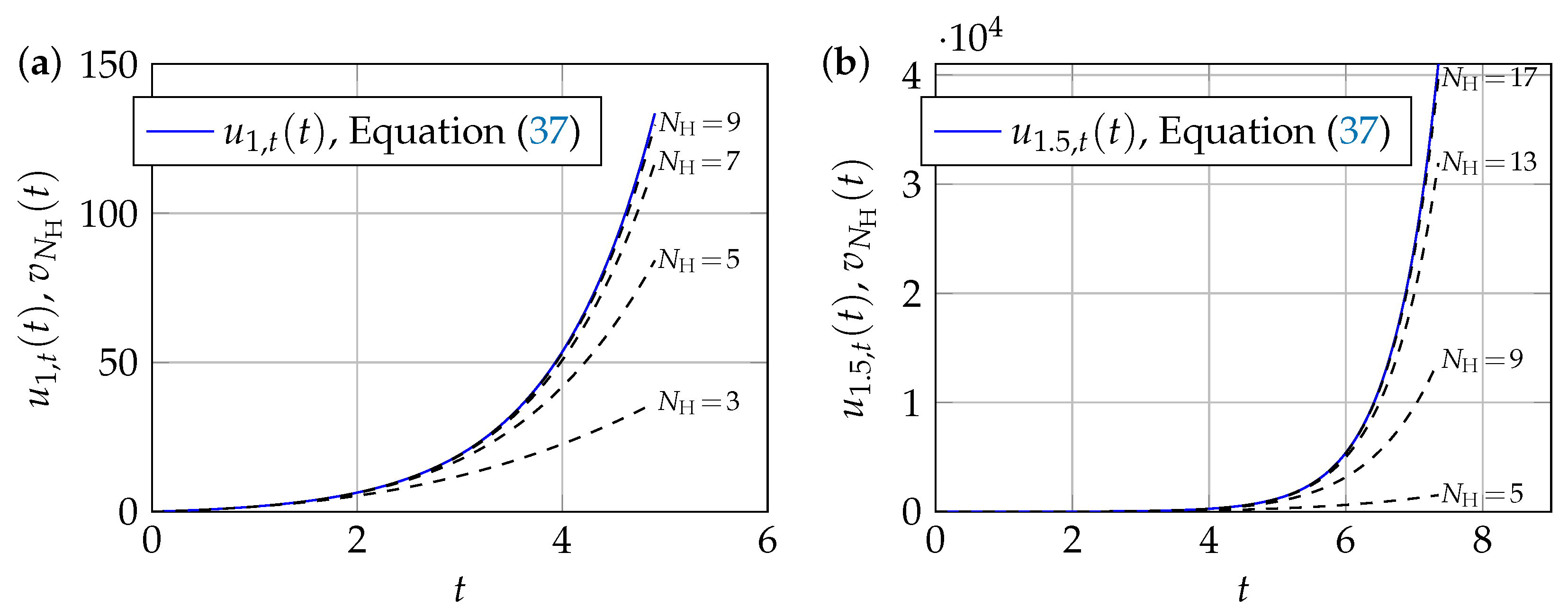
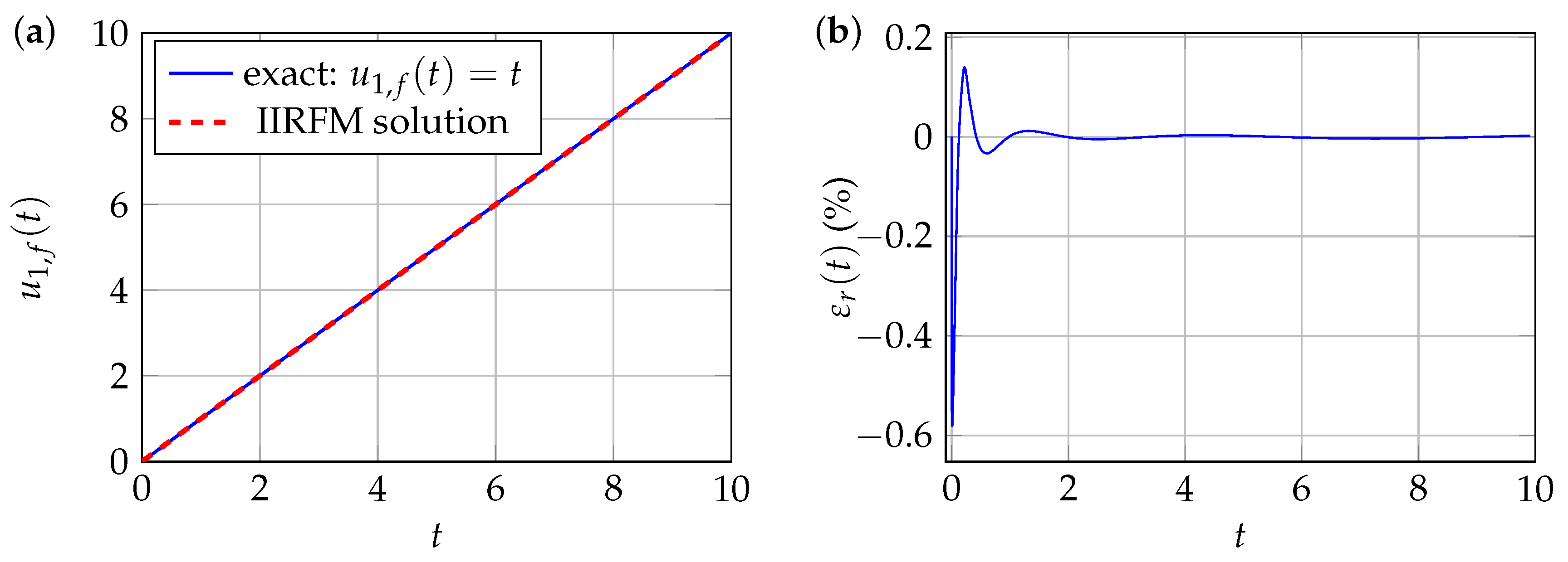
3.1.1. Monomial Source Term $f\left(t\right)=t^n$

We first consider a monomial source term $f\left(t\right)=t^n$, which leads to a relatively simple analytical expression for the solution, denoted here by $u_{\lambda ,t^n}\left(t\right)$:

$$u_{\lambda ,t^n}\left(t\right)=t^n\left\{1+{\displaystyle \frac{e^{\lambda t}}{{\left(\lambda t\right)}^n}}\left[\Gamma (n+1)-\Gamma (n+1,\lambda t)\right]\right\},$$

(37)

where $\Gamma (n,z)={\int }_z^{\infty }{x}^{n-1}{e}^{-x}\mathrm{d}x$ is the incomplete gamma function and $\Gamma (n+1)=\Gamma (n+1,0)$. For $t\in {\mathbb{R}}^{+}$ and $n\in \mathbb{N}$, Equation (37) admits the following Maclaurin series expansion:

$$u_{\lambda ,t^n,m}\left(t\right)=t^n+{\displaystyle \frac{\lambda t^{n+1}}{n+1}}+{\displaystyle \frac{{\lambda }^2{t}^{n+2}}{\left(n+1\right)\left(n+2\right)}}+\cdots +{\displaystyle \frac{{\lambda }^m{t}^{m+n}}{\left(n+1\right)\cdots \left(n+m\right)}}+O\left(t^{m+n+1}\right).$$

(38)

Note that in the special case where $n=1$, the analytical solution $u_{\lambda ,t}\left(t\right)$ is given by the following expression, deduced from (37):

$$u_{\lambda ,t}\left(t\right)={\displaystyle \frac{e^{\lambda t}-1}{\lambda }},$$

(39)

whose limit for $t\to \infty$ tends to $1/\left|\lambda \right|$ when $\lambda <0$.

Numerical Solution by the IIRFM

The application of the IIRFM presented in Section 2.1, leads in the present case to the following relations, with $\overline{K}\left(s\right)=1/s$ and $H_{\mathrm{L}}(s,\lambda )=s/(s-\lambda )$:

$$\mathcal{L}\left[u_{\lambda ,f}\left(t\right)\right]=H_{\mathrm{L}}(s,\lambda )\mathcal{L}\left[f\left(t\right)\right]\Rightarrow \mathcal{L}\left[u_{\lambda ,f}\left(t\right)\right]={\displaystyle \frac{s}{s-\lambda }}\mathcal{L}\left[f\left(t\right)\right].$$

(40)

For the case $f\left(t\right)=t^n$, one finds $\mathcal{L}\left[f\left(t\right)\right]=\Gamma \left(n+1\right)s^{-(n+1)}$, in which case it is possible to analytically invert the Laplace transform (40), giving back the analytical result (37).

Rather than an analytical solution, we are looking here for a numerical solution, designated by $u_{\lambda ,f}^{\mathrm{IIR}}$, deduced from relation (40). To this end, the bilinear transformation $s\to {\displaystyle \frac{2}{T_e}}{\displaystyle \frac{z-1}{z+1}}$ is applied to the Laplace transfer function $H_{\mathrm{L}}(s,\lambda )=s/(s-\lambda )$, without having to calculate the Laplace transform of the source function $f\left(t\right)$. The application of the bilinear transformation leads to the following z-transfer function:

$$H_{\mathrm{L}}(z,\lambda )={\displaystyle \frac{{\overline{u}}_{\lambda ,f}^{\mathrm{IIR}}\left(z\right)}{\overline{f}\left(z\right)}}={\displaystyle \frac{1-z^{-1}}{\left(1-\frac{\lambda T_e}{2}\right)-\left(1+\frac{\lambda T_e}{2}\right)z^{-1}}}.$$

(41)

Using time-shifting properties $\mathrm{TZ}\left[x\left((k-m)T_e\right)\right]=z^{-m}\mathrm{TZ}\left[x\left(k{T}_e\right)\right]$ and linearity $\mathrm{TZ}\left[a_{m}x\left(k{T}_e\right)\right]=a_m\mathrm{TZ}\left[x\left(k{T}_e\right)\right]$ of the z-transform, we obtain the recurrence relation satisfied by the solution $u_{\lambda ,f}^{\mathrm{IIR}}\left(t_k\right)$ at the following discrete time $t_k=k{T}_e$:

$$u_{\lambda ,f}^{\mathrm{IIR}}\left(t_k\right)={\displaystyle \frac{1+\frac{\lambda T_e}{2}}{1-\frac{\lambda T_e}{2}}}{u}_{\lambda ,f}^{\mathrm{IIR}}\left(t_{k-1}\right)+{\displaystyle \frac{f\left(t_k\right)-f\left(t_{k-1}\right)}{1-\frac{\lambda T_e}{2}}},$$

(42)

where $u_{\lambda ,f}^{\mathrm{IIR}}\left(t_0\right)=0$ and $T_e\in {\mathbb{R}}^{+}$ is the sample period, satisfying $T_e\ne 2/\left|\lambda \right|$.

In the specific case $f\left(t\right)=t^n$ considered in this paragraph, $f\left(t_k\right)-f\left(t_{k-1}\right)$ can be assimilated to $T_e{f}^{\prime }\left(t_k\right)=n{T}_e^n{k}^{n-1}$. It is then possible to derive an approximate explicit expression of $u_{\lambda ,t^n}^{\mathrm{IIR}}\left(t_k\right)$, which will be denoted by ${\tilde{u}}_{\lambda ,t^n}^{\mathrm{IIR}}\left(t_k\right)$

$${\tilde{u}}_{\lambda ,t^n}^{\mathrm{IIR}}\left(t_k\right)=n{T}_e^n\left[{\displaystyle \frac{w^{-k}{\mathrm{Li}}_{1-n}\left(w\right)}{1-\frac{\lambda T_e}{2}}}-{\displaystyle \frac{\Phi \left(w,1-n,k+1\right)}{1+\frac{\lambda T_e}{2}}}\right],$$

(43)

where $w=(2-\lambda T_e)/(2+\lambda T_e)$; ${\mathrm{Li}}_m\left(w\right)={\sum }_{p=1}^{\infty }{w}^p/p^m$ is the polylogarithm function and $\Phi \left(w,a,b\right)={\sum }_{p=0}^{\infty }{w}^p/{(p+b)}^a$ is the Lerch transcendent function. These two functions are analytically extended for $\left|w\right|>1$.

Exact Solution by Homotopic Perturbation Method with Laplace Transformation (HPM-L)

The application of the HPM-L method presented in Section 2.2 leads in the present case to the following relationships, deduced from results (35) and from the Laplace transform $\mathcal{L}\left(t^n\right)=\Gamma (n+1)/s^{n+1}$:   

$$\left|\begin{array}{cc}0:& v_0\left(t\right)=t^n,\\ 1:& v_1\left(t\right)=\lambda {\mathcal{L}}^{-1}\left[\mathcal{L}\left(t^n\right)s^{-1}\right]=\lambda \Gamma (n+1){\mathcal{L}}^{-1}\left(s^{-n-2}\right)=\lambda {\displaystyle \frac{\Gamma (n+1)}{\Gamma (n+2)}}{t}^{n+1},\\ & \Rightarrow v_1\left(t\right)={\displaystyle \frac{\lambda t^{n+1}}{n+1}},\\ 2:& v_2\left(t\right)=\lambda {\mathcal{L}}^{-1}\left[\mathcal{L}\left({\displaystyle \frac{\lambda t^{n+1}}{n+1}}\right)s^{-1}\right]={\displaystyle \frac{{\lambda }^2}{n+1}}\Gamma (n+2){\mathcal{L}}^{-1}\left(s^{-n-3}\right)={\displaystyle \frac{{\lambda }^2}{n+1}}{\displaystyle \frac{\Gamma (n+2)}{\Gamma (n+3)}}{t}^{n+2},\\ & \Rightarrow v_2\left(t\right)={\displaystyle \frac{{\lambda }^2{t}^{n+2}}{\left(n+1\right)\left(n+2\right)}},\\ ⋮& ⋮\\ m:& v_m\left(t\right)=\lambda {\mathcal{L}}^{-1}\left\{\mathcal{L}\left[{\displaystyle \frac{{\lambda }^{m-1}{t}^{n+m-1}}{\left(n+1\right)\left(n+2\right)\cdots \left(n+m-1\right)}}\right]s^{-1}\right\}={\displaystyle \frac{{\lambda }^m}{\left(n+1\right)\left(n+2\right)\cdots \left(n+m-1\right)}}{\displaystyle \frac{\Gamma (n+m)}{\Gamma (n+m+1)}}{t}^{n+m},\\ & \Rightarrow v_m\left(t\right)={\displaystyle \frac{{\lambda }^m{t}^{n+m}}{\left(n+1\right)\cdots \left(n+m\right)}},\\ ⋮& ⋮\end{array}\right.$$

The $v\left(t\right)$ solution obtained by the HPM-L method is therefore written here, according to relation (32)

$$\begin{array}{cc}\hfill v\left(t\right)& =t^n+{\displaystyle \frac{\lambda t^{n+1}}{n+1}}+{\displaystyle \frac{{\lambda }^2{t}^{n+2}}{\left(n+1\right)\left(n+2\right)}}+\cdots +{\displaystyle \frac{{\lambda }^m{t}^{n+m}}{\left(n+1\right)\cdots \left(n+m\right)}}+\cdots ,\hfill \\ \hfill & =n!t^n\sum _{m=0}^{\infty }{\displaystyle \frac{{\left(\lambda t\right)}^m}{\left(n+m\right)!}}.\hfill \end{array}$$

(44)

Since ${\sum }_{m=1}^{\infty }{\displaystyle \frac{{\left(\lambda t\right)}^m}{\left(n+m\right)!}}=e^{\lambda t}{\left(\lambda t\right)}^{-n}\left[\Gamma (n+1)-\Gamma (n+1,\lambda t)\right]/\Gamma (n+1)$, we find analytical result (37).

Approximate Numerical Solutions for $f\left(t\right)=t$

The approximate numerical solutions obtained by the HPM-L and IIRFM methods, respectively, are now compared in the case where $f\left(t\right)=t$.

The HPM-L approximate numerical solution is obtained by truncating (44) at rank $N_{\mathrm{H}}$. Table 1 shows the absolute errors ${\epsilon }_{N_{\mathrm{H}}}^{\infty }\left(5\right|\lambda \left|\right)=|u_{\lambda ,t}\left(5\right|\lambda \left|\right)-v_{N_{\mathrm{H}}}\left(5\right|\lambda \left|\right)|$ obtained when $t=5\left|\lambda \right|$, between the analytical value $u_{\lambda ,t}\left(5\right|\lambda \left|\right)$ and the approximation $v_{N_{\mathrm{H}}}\left(5\right|\lambda \left|\right)$, for different values of $N_{\mathrm{H}}$, when the parameter $\lambda$ takes the values $\pm 0.5,\pm 1.0$ and $\pm 1.5$.

Table 1. Influence of $\lambda$ parameter on absolute error ${\epsilon }_{N_{\mathrm{H}}}^{\infty }\left(5\right|\lambda \left|\right)=|u_{\lambda ,t}\left(5\right|\lambda \left|\right)-v_{N_{\mathrm{H}}}\left(5\right|\lambda \left|\right)|$ committed at $t=5\left|\lambda \right|$ with the HPM-L method, when $K(t,t^{\prime })=1$, $f\left(t\right)=t$ and for different values of $N_{\mathrm{H}}$. Numbers in parentheses indicate multiplying powers of ten.

${\mathit{N}}_{\mathbf{H}}$=	3	5	7	15	20	30
$\left|\lambda \right|=0.5$	$2.67144(-1)$	$1.28311(-2)$	$3.42505(-4)$	$3.66374(-12)$	$8.88178(-16)$	-
$\left|\lambda \right|=1.0$	$1.09080(+1)$	$5.69965(+1)$	$1.97941(+1)$	$1.02417(-2)$	$1.20352(-5)$	$6.82121(-13)$
$\left|\lambda \right|=1.5$	$5.10447(+4)$	$4.95956(+4)$	$4.47047(+4)$	$5.46097(+3)$	$3.04954(+2)$	$4.77714(-2)$

For $\left|\lambda \right|=0.5,1.0$, and $1.5$, the results gathered in Table 1 show that the absolute error ${\epsilon }_{N_{\mathrm{H}}}^{\infty }\left(5\right|\lambda \left|\right)$ is less than 0.01 for the respective truncation orders $N_{\mathrm{H}}⩾6,16$, and 32. These results (as well as all the other results gathered in Table 1) show the influence of the value of $\lambda$ on the speed of convergence of the HPM-L method. In particular, the larger the value of $\left|\lambda \right|$, the slower the convergence of the HPM-L method here. Figure 3a,b shows the evolution of the approximate solution $v_{N_{\mathrm{H}}}\left(t\right)$ as a function of t, for $n=1$ and, respectively, for $\lambda =1$ and $\lambda =1.5$, for different values of $N_{\mathrm{H}}$. The numerical results (dashed curves) provided by the HPM-L method are compared with the analytical solutions (solid curves) $u_{1,t}\left(t\right)$ and $u_{1.5,t}\left(t\right)$. These figures clearly show that the number $N_{\mathrm{H}}$ of terms, required to obtain an approximate solution $v_{N_{\mathrm{H}}}\left(t\right)$ converging to the analytical solution $u_{\lambda ,1}\left(t\right)$, increases with the value of $\lambda$. From a numerical point of view, this can be a definite handicap for the HPM-L approach, especially when there is no closed form of the solution.

Figure 3. Dashed lines show the evolution of $v_{N_{\mathrm{H}}}\left(t\right)$ as a function of t for $n=1$, different values of $\lambda$, and different values of $N_{\mathrm{H}}$: (a) $\lambda =1$ and $N_{\mathrm{H}}=3,5,7,9$; (b) $\lambda =1.5$ and $N_{\mathrm{H}}=5,9,13,17$.

We are now looking for the numerical solution ${\tilde{u}}_{\lambda ,f}^{\mathrm{IIR}}\left(t_k\right)$ at $t_k=k{T}_e$, using the IIRFM. In the case of a unit kernel and for $f\left(t\right)=t$, result (43) takes on the following expression, valid whatever the sign of $\lambda$:

$${\tilde{u}}_{\lambda ,t}^{\mathrm{IIR}}\left(t_k\right)={\displaystyle \frac{1}{\lambda }}{\left({\displaystyle \frac{2+\lambda T_e}{2-\lambda T_e}}\right)}^k-{\displaystyle \frac{1}{\lambda }}.$$

(45)

This is a particularly simple expression, whose accuracy depends, for a given value of $\lambda$, on the choice of the value of $T_e$. Note that ${lim}_{t_k\to \infty }{\tilde{u}}_{\lambda ,t}^{\mathrm{IIR}}\left(t_k\right)\to 1/\left|\lambda \right|$ when $\lambda <0$, which is consistent with the exact result of (39). Table 2 gathers the absolute errors ${\epsilon }_{T_e}^{\infty }\left(5\right|\lambda \left|\right)=|u_{\lambda ,t}\left(5\right|\lambda \left|\right)-{\tilde{u}}_{\lambda ,t}^{\mathrm{IIR}}\left(5\right|\lambda \left|\right)|$ obtained when $t_k=5\left|\lambda \right|$, between the analytical value $u_{\lambda ,t}\left(5\right|\lambda \left|\right)$ and the approximate result ${\tilde{u}}_{\lambda ,t}^{\mathrm{IIR}}\left(5\right|\lambda \left|\right)$, for different values of $T_e$, when $\lambda$ takes the values $\pm 0.5,\pm 1.0$, and $\pm 1.5$.

Table 2. Influence of $\lambda$ on absolute error ${\epsilon }_{T_e}^{\infty }\left(5\right|\lambda \left|\right)=|u_{\lambda ,t}\left(5\right|\lambda \left|\right)-{\tilde{u}}_{\lambda ,t}^{\mathrm{IIR}}\left(5\right|\lambda \left|\right)|$ at $t_k=5\left|\lambda \right|$ using IIRFM, when $\alpha =0$, $f\left(t\right)=t$ and different values of $T_e$. Numbers in parentheses indicate multiplying powers of ten.

${\mathit{T}}_{\mathit{e}}$=	${10}^{-1}$	${10}^{-3}$	${10}^{-5}$	${\mathit{T}}_{\mathit{e}}$=	${10}^{-1}$	${10}^{-3}$	${10}^{-5}$
$\lambda =-0.5$	$1.49258(-4)$	$1.49218(-8)$	$1.50691(-11)$	$\lambda =0.5$	$1.81881(-3)$	$1.8179(-7)$	$1.32737(-10)$
$\lambda =-1.0$	$2.80584(-5)$	$2.80777(-9)$	$2.58013(-11)$	$\lambda =1.0$	$6.20611(-1)$	$6.18386(-5)$	$2.5262(-8)$
$\lambda =-1.5$	$1.81606(-7)$	$1.81704(-11)$	$3.11284(-12)$	$\lambda =1.5$	$1.09635(+3)$	$1.08113(-1)$	$8.04227(-6)$

The analysis of the results gathered in Table 2 shows that the IIRFM leads to highly accurate results for negative values of $\lambda$, even for sampling periods as large as $T_e=0.1$. This is a very interesting result. As Equation (45) is simpler than Equation (39), which includes the incomplete gamma special function, it is also easier to implement numerically, and poses no particular convergence problems.

Figure 4 shows the variations of relative errors ${\epsilon }_r^{\mathrm{NM}}\left(t\right)=|u^{\mathrm{NM}}\left(t\right)/u_{\lambda ,t}\left(t\right)-1|$ as a function of t, where (NM) stands for “numerical method”, with NM≡HPM-L or IIRFM. The value of $\lambda$ is negative here and equals $\lambda =-1.5$. The calculation step is the same for both numerical approaches and is equal to $\delta t=T_e={10}^{-2}$. For $N_{\mathrm{H}}=15$, we can clearly see from Figure 4 that the IIRFM performs significantly better than the HPM-L method as t deviates from zero.

Figure 4. Relative errors as a function of t, when $\alpha =0$, $f\left(t\right)=t$, and $\lambda =-1.5$: (a) ${\epsilon }_r^{\mathrm{HPM}-\mathrm{L}}\left(t\right)$ with $N_{\mathrm{H}}=15$ and $T_e={10}^{-2}$; (b) ${\epsilon }_r^{\mathrm{IIRFM}}\left(t\right)$ with $T_e={10}^{-2}$.

Since $v_{N_{\mathrm{H}}}\left(t\right)$ has the same form as the Maclaurin series expansion (38), the approximate solution provided by the HPM-L method is very accurate in the vicinity of $t=0$, as shown in Figure 4a, even for small values of $N_{\mathrm{H}}$. In contrast, as soon as t deviates from the origin, the number $N_{\mathrm{H}}$ of terms required to obtain a precise numerical value must increase accordingly, which can prove to be a problem from the point of view of numerical calculation (particularly in terms of calculation time). The numerical behavior of the IIRFM is very different from that of the HPM-L method. Indeed, as shown in Figure 4b, the accuracy of (45) increases with $t_k=k{T}_e$ when $\lambda <0$.

Figure 5 shows the variations in the relative errors ${\epsilon }_r^{\mathrm{HPM}-\mathrm{L}}\left(t\right)$ and ${\epsilon }_r^{\mathrm{IIRFM}}\left(t\right)$ as a function of t, when the parameter $\lambda$ is positive and equal to $\lambda =1.5$, with all other quantities having the same values as those used for Figure 4. Even though the accuracy of the IIRFM decreases this time as $t_k$ deviates from the origin, it remains more accurate than the HPM-L method.

Figure 5. Relative errors as a function of t, when $K(t,t^{\prime })=1$, $f\left(t\right)=t$, and $\lambda =1.5$: (a) ${\epsilon }_r^{\mathrm{HPM}-\mathrm{L}}\left(t\right)$ with $N_{\mathrm{H}}=15$ and $T_e={10}^{-2}$; (b) ${\epsilon }_r^{\mathrm{IIRFM}}\left(t\right)$ with $T_e={10}^{-2}$.

The order of accuracy n of the IIRFM approximation can be evaluated by computing the absolute value of the difference ${\tilde{u}}_{\lambda ,t}^{\mathrm{IIR}}\left(t_k\right)-u_{\lambda ,t}\left(t_k\right)$, as a function of the sampling period $T_e$. Using the expressions (39) and (45), we obtain

$${\epsilon }_k\left(T_e\right)=\left|{\tilde{u}}_{\lambda ,t}^{\mathrm{IIR}}\left(t_k\right)-u_{\lambda ,t}\left(t_k\right)\right|={\displaystyle \frac{1}{\left|\lambda \right|}}\left|e^{k\lambda T_e}-{\left({\displaystyle \frac{2+\lambda T_e}{2-\lambda T_e}}\right)}^k\right|.$$

(46)

Figure 6 shows the evolution of ${\epsilon }_k\left(T_e\right)$ as a function of $T_e\in [{10}^{-5},{10}^{-1}]$, when $t_k=1$ and $\lambda =1$. It can be seen from Figure 6 that the IIRFM approach is a second-order accuracy method in the present case.

Figure 6. Absolute error ${\epsilon }_k\left(T_e\right)$ as a function of $T_e$, when $K(t,t^{\prime })=1$, $f\left(t\right)=t$, $\lambda =1$, and $t_k=1$.

In conclusion, it should be noted that, whatever the sign of $\lambda$, the accuracy of the IIRFM can be improved by reducing $T_e$. This is not the case with the results obtained by the HPM-L method, whose accuracy is independent of $T_e$.

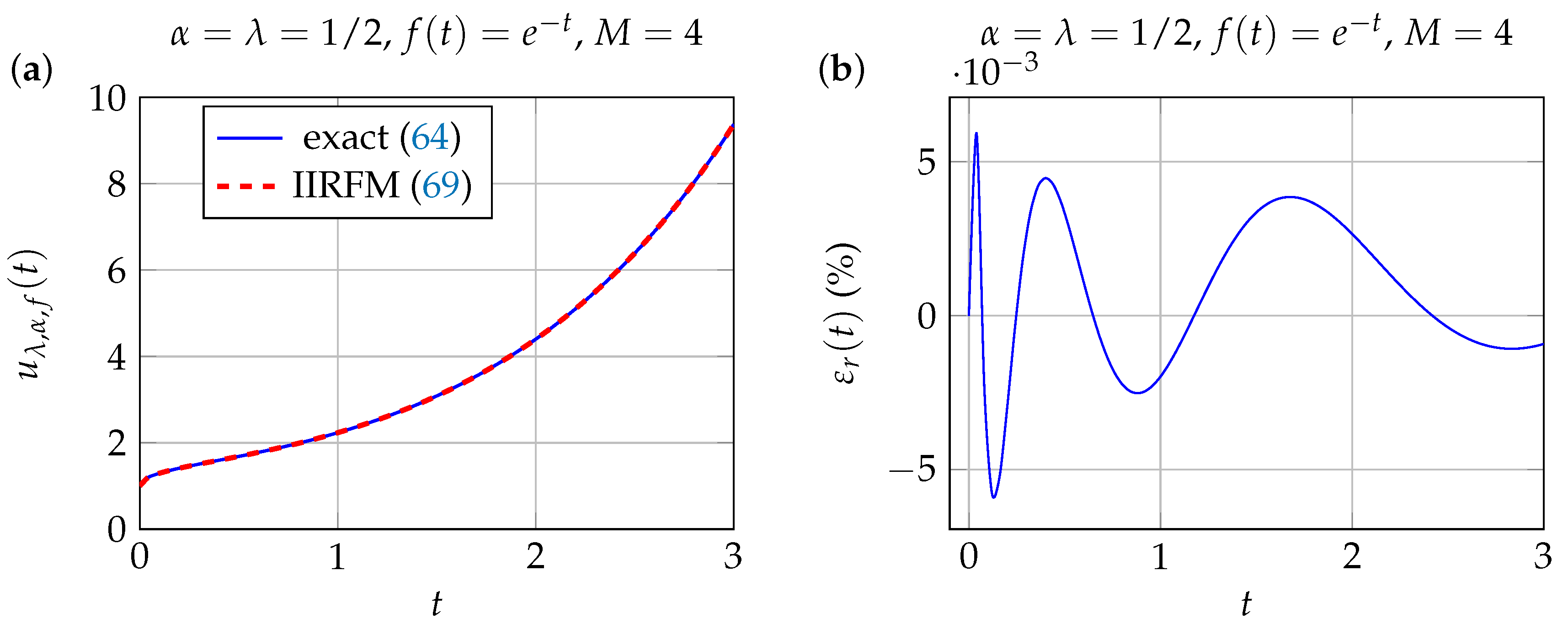
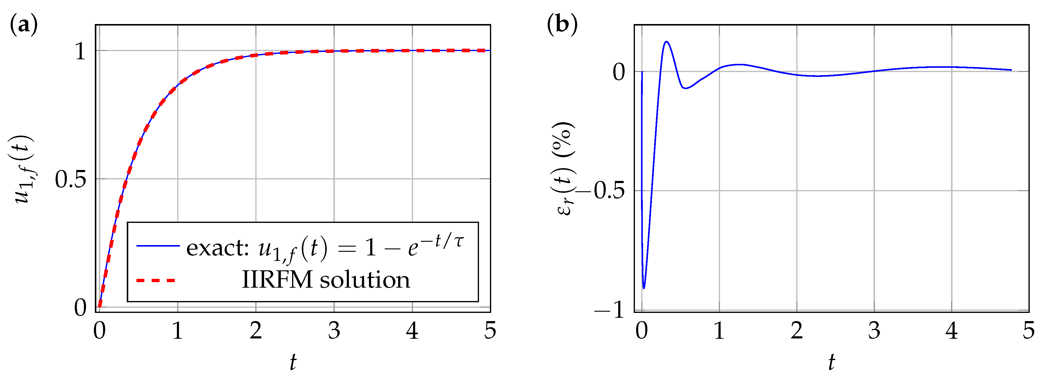
3.1.2. Exponential Source Term $f\left(t\right)=e^{-t}$

As a preamble to this paragraph, it should be noted that it is not necessary for the initial condition on the solution to be null in order to apply the IIRFM in the case of the unit kernel.

The developments of the previous paragraph are repeated, but this time in the case of a source term $f\left(t\right)$ of exponential form. In this case, there is also an analytical solution $u_{\lambda ,e^{-t}}\left(t\right)$ of Equation (3), which is

$$u_{\lambda ,e^{-t}}\left(t\right)=\left|\begin{array}{c}{\displaystyle \frac{e^{-t}+\lambda e^{\lambda t}}{1+\lambda }}\mathrm{when}\lambda \ne -1,\hfill \\ (1-t)e^{-t}\mathrm{when}\lambda =-1.\hfill \end{array}\right.$$

(47)

The most general case, where $\lambda \ne -1$, is considered in the following. For $t\in {\mathbb{R}}^{+}$, Equation (47) admits a Maclaurin series expansion $u_{\lambda ,e^{-t},m}\left(t\right)$ of the following form to order m:

$$u_{\lambda ,e^{-t},m}\left(t\right)=\sum _{n=0}^m{\displaystyle \frac{{(-1)}^m+{\lambda }^{m+1}}{(\lambda +1)m!}}{t}^m+O\left(t^{m+1}\right).$$

(48)

Numerical Solution by the IIRFM

Since the transfer function $H(z,\lambda )$ associated with Equation (3) is independent of the source function $f\left(t\right)$, the numerical solution $u_{\lambda ,e^{-t}}^{\mathrm{IIR}}$ of the present problem still verifies recurrence relation (42). Equating the difference $f\left(t_k\right)-f\left(t_{k-1}\right)$ with the function $T_e{f}^{\prime }\left(t_k\right)=-T_e{e}^{-k{T}_e}$, it is also possible to find here an approximate explicit expression for the series $u_{\lambda ,e^{-t}}^{\mathrm{IIR},T_e}\left(t_k\right)$, an expression which is denoted by ${\tilde{u}}_{\lambda ,e^{-t}}^{\mathrm{IIR}}\left(t_k\right)$, as follows:

$${\tilde{u}}_{\lambda ,e^{-t}}^{\mathrm{IIR},T_e}\left(t_k\right)={\displaystyle \frac{e^{-t_k}{\omega }^{\prime }-\left(1+\frac{{\omega }^{\prime }}{\omega }\right){\omega }^{1-t_k/T_e}+e^{T_e}{\omega }^{-t_k/T_e}}{e^{T_e}-\omega }},$$

(49)

where $\omega =(2-\lambda T_e)/(2+\lambda T_e)$, and ${\omega }^{\prime }=2T_e/(2+\lambda T_e)$, with $T_e\ne -2/\lambda$. Note that here ${\tilde{u}}_{\lambda ,e^{-t}}^{\mathrm{IIR},T_e}\left(0\right)=f\left(0\right)=1$.

Solution by the HPM-L Method

The application of the HPM-L method leads to the following relationships:

$$\left|\begin{array}{cc}0:& v_0\left(t\right)=e^{-t},\\ 1:& v_1\left(t\right)=\lambda {\mathcal{L}}^{-1}\left[\mathcal{L}\left(e^{-t}\right)s^{-1}\right]=\lambda {\mathcal{L}}^{-1}\left({\displaystyle \frac{1}{s+s^2}}\right),\\ & \Rightarrow v_1\left(t\right)=\lambda \left(1-e^{-t}\right),\\ 2:& v_2\left(t\right)=\lambda {\mathcal{L}}^{-1}\left\{\mathcal{L}\left[\lambda \left(1-e^{-t}\right)\right]s^{-1}\right\}={\lambda }^2{\mathcal{L}}^{-1}\left({\displaystyle \frac{1}{s^2}}-{\displaystyle \frac{1}{s+s^2}}\right),\\ & \Rightarrow v_2\left(t\right)={\lambda }^2\left(t-1+e^{-t}\right),\\ 3:& v_3\left(t\right)=\lambda {\mathcal{L}}^{-1}\left\{\mathcal{L}\left[{\lambda }^2\left(t-1+e^{-t}\right)\right]s^{-1}\right\}={\lambda }^3{\mathcal{L}}^{-1}\left({\displaystyle \frac{1}{s^3}}-{\displaystyle \frac{1}{s^2}}+{\displaystyle \frac{1}{s+s^2}}\right),\\ & \Rightarrow v_3\left(t\right)={\lambda }^3\left(1-t+{\displaystyle \frac{1}{2}}{t}^2-e^{-t}\right),\\ ⋮& ⋮\\ m:& v_m\left(t\right)=\lambda {\mathcal{L}}^{-1}\left\{\mathcal{L}\left[{\lambda }^{m-1}\left({(-1)}^{m-2}\sum _{k=0}^{m-2}{\displaystyle \frac{{(-1)}^k}{k!}}{t}^k+{(-1)}^{m-1}{e}^{-t}\right)\right]s^{-1}\right\},\\ & ={\lambda }^m{\mathcal{L}}^{-1}\left[{(-1)}^{m-2}\sum _{k=0}^{m-2}{\displaystyle \frac{{(-1)}^k}{s^{k+2}}}+{\displaystyle \frac{{(-1)}^{m-1}}{s+s^2}}\right],\\ & \Rightarrow v_m\left(t\right)={\lambda }^m\left[{(-1)}^{m-1}\sum _{k=0}^{m-1}{\displaystyle \frac{{(-1)}^k}{k!}}{t}^k+{(-1)}^m{e}^{-t}\right],\\ ⋮& ⋮\end{array}\right.$$

(50)

The solution $v\left(t\right)$ obtained by the HPM-L method is therefore written here, according to equations (32) and (50):

$$v\left(t\right)=\sum _{m=0}^{\infty }{v}_m\left(t\right)=\sum _{m=0}^{\infty }{\lambda }^m\left[{(-1)}^{m-1}\sum _{k=0}^{m-1}{\displaystyle \frac{{(-1)}^k}{k!}}{t}^k+{(-1)}^m{e}^{-t}\right].$$

(51)

An approximate form of the solution, denoted by $v_{N_{\mathrm{H}}}\left(t\right)$, is obtained by truncating series (51) at a rank $N_{\mathrm{H}}<\infty$.

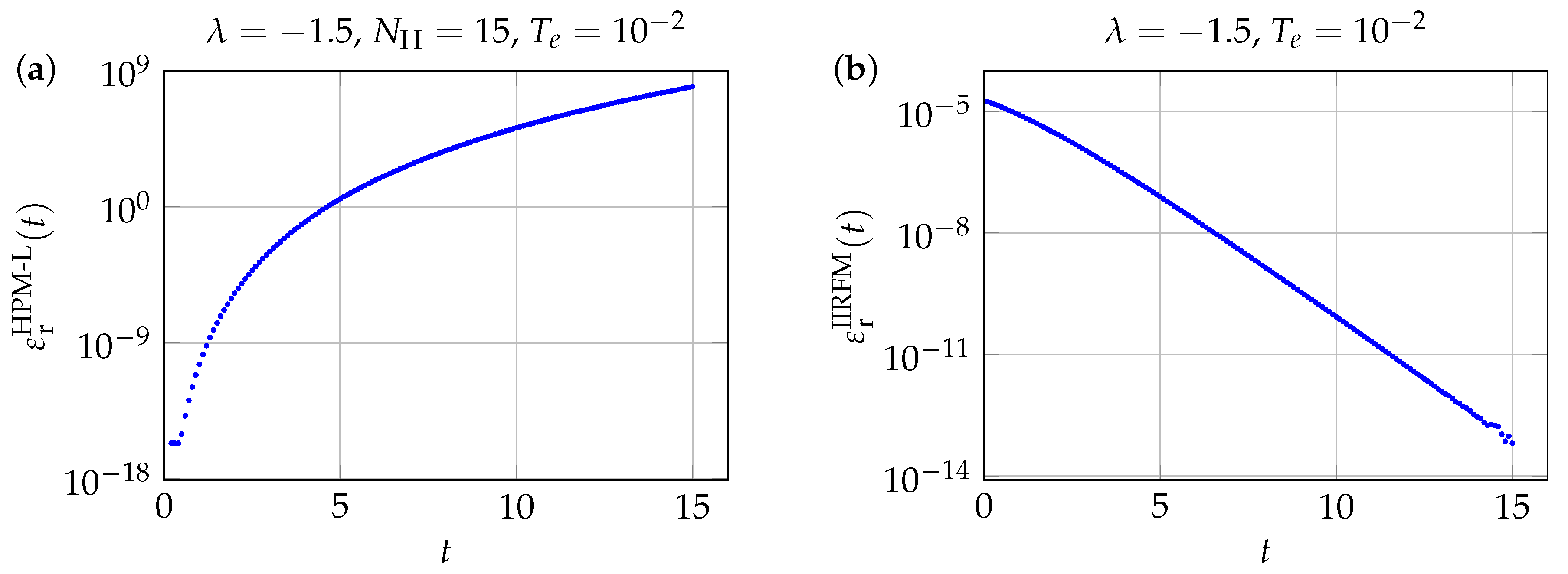
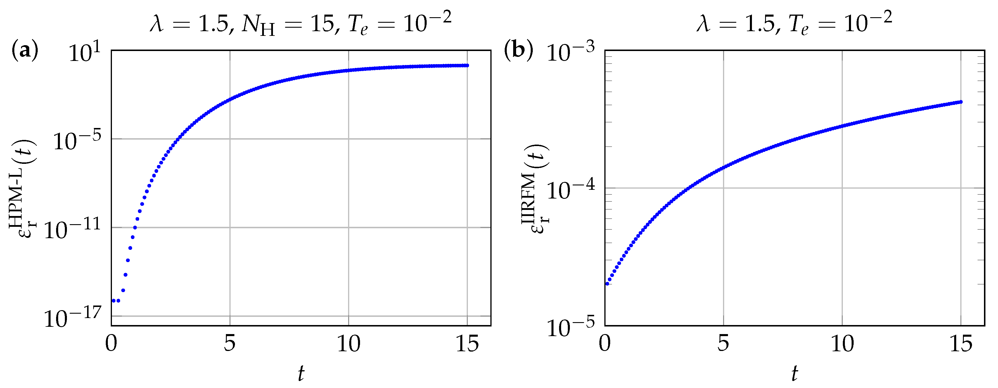
Numerical Results and Discussion

Figure 7a represents the numerical results obtained by the HPM-L (result (51)) and IIRFM (result (49)) methods, for $f\left(t\right)=e^{-t}$, $\lambda =5$, $T_e={10}^{-2}$, and $t\in I_t=[0,5]$, using the semi-logarithmic representation. It can be seen that relatively high $N_{\mathrm{H}}$ truncation orders have to be used for the numerical solution $v_{N_{\mathrm{H}}}\left(t\right)$ provided by the HPM-L method to converge to the exact solution (47) with acceptable accuracy over the entire interval $I_t$. In contrast, it is observed that the numerical solution ${\tilde{u}}_{\lambda ,e^{-t}}^{\mathrm{IIR},T_e}$ provides a very accurate approximation of the exact solution $u_{\lambda }\left(t\right)$ over the entire interval $I_t=[0,5]$, even for a time step as large as $T_e={10}^{-2}$.

Figure 7. IIRFM and HPM-L numerical results when $K(t,t^{\prime })=1$, $f\left(t\right)=e^{-t}$, $T_e={10}^{-2}$, and $N_{\mathrm{H}}=5,15$, and 20: (a) $\lambda =5$ and (b) $\lambda =-5$.

The observations made in the previous discussion for $\lambda =5$ are even more evident when the value $\lambda =-5$ is chosen. As shown in Figure 7b, convergence of the HPM-L method is slow in the case where $\lambda =-5$. In the present case, no finite value of $N_{\mathrm{H}}$ could be found that allows the series $v_{N_{\mathrm{H}}}\left(t\right)$ to converge to the exact solution $u_{\lambda ,e^{-t}}\left(t\right)$ on the interval $I_t=[0,5]$ without using a convergence acceleration procedure. In contrast, we can observe that the IIRFM approach again gives a very accurate numerical approximation on $I_t$, whatever the value of $\lambda$. It was also observed that the HPM-L method became unusable here from a numerical point when $\lambda ⩽-10$.

In the present case, the IIRFM approach was found to be a first-order accuracy method.

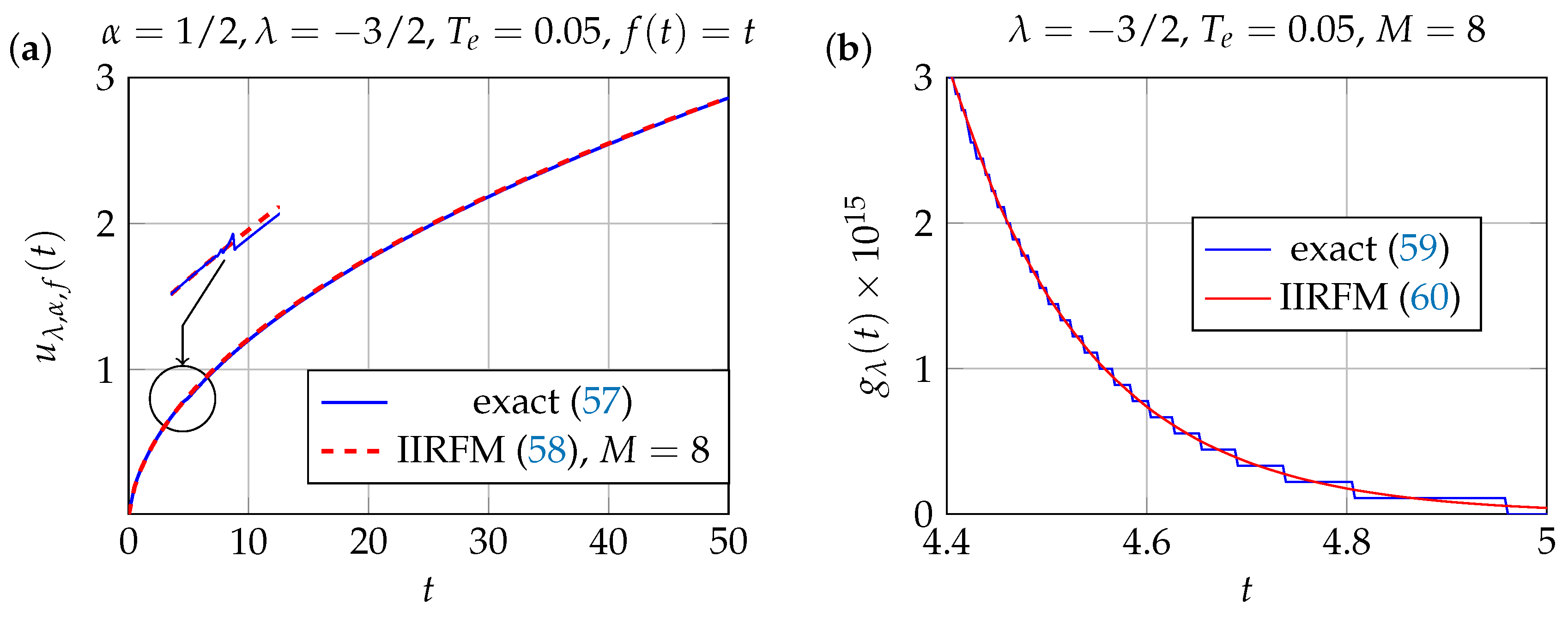
3.2. Abel’s Kernel (with $\alpha =1/2$)

In the case of Abel’s kernel, one obtains $\overline{K}\left(s\right)=\Gamma (1-\alpha )/s^{1-\alpha }$, and the transfer function $H_{\mathrm{L}}(s,\lambda )$ is then given by

$$H_{\mathrm{L}}(s,\lambda )={\displaystyle \frac{1}{1-\lambda \Gamma (1-\alpha )s^{\alpha -1}}}.$$

(52)

The results of Section 2 are applied here to the case $\alpha =1/2$, for different source terms $f\left(t\right)$ and different values of the parameter $\lambda$. Only the IIRFM approach is developed in detail in this section. To differentiate the results of this paragraph from those obtained in the previous paragraph for $K(t,t^{\prime })=1$, we now agree to index all useful functions by the value of $\alpha$.

In the present case, the Laplace transfer function $H_{\mathrm{L},{\displaystyle \frac{1}{2}}}(s,\lambda )$ of Abel’s problem is given, from Equation (17), by

$$H_{\mathrm{L},{\displaystyle \frac{1}{2}}}(s,\lambda )={\displaystyle \frac{\sqrt{s}}{\sqrt{s}-\lambda \sqrt{\pi }}}.$$

(53)

In contrast to the case where $K(t,t^{\prime })=1$ studied in Section 3.1, there is no exact expression here for $H_{\mathrm{L},{\displaystyle \frac{1}{2}}}(s,\lambda )$ in the form of a quotient of polynomials in s. To apply the IIRFM in the present case, the function $G_{{\displaystyle \frac{1}{2}}}(s,\lambda )=H_{\mathrm{L},{\displaystyle \frac{1}{2}}}(s,\lambda )-1$ needs to be approximated by a rational fraction as accurate as possible. Several approaches make obtaining this approximation possible. In [23], an approximation of the transfer function was obtained using the least-squares method, while in [11,24] the rational fraction was constructed using Padé approximants. The second approach generally allows the construction of a very precise rational fraction, but mainly in the vicinity of a given point of the Laplace space. In order to obtain an accurate description over an extended domain of the Laplace space, and thus over an extended domain of the direct time space, a Chebyshev rational interpolation of the function $G_{{\displaystyle \frac{1}{2}}}(s,\lambda )$, has been carried out here over a suitably chosen interpolation interval $I_s=[s_i,s_f]$. The $I_s$ interval is adjusted to obtain the best possible numerical resolution of Equation (3) over the entire time domain. This makes it possible to predict, with comparable accuracies, the behaviors of the solution of Equation (3) at both long and short times.

3.2.1. IIRFM Approach When $\alpha =1/2$ and $\lambda ⩽0$

Situations where $\lambda ⩽0$ are first considered. In this case, the denominator of the exact transfer function $H_{\mathrm{L},{\displaystyle \frac{1}{2}}}(s,\lambda )$ has no root with a positive real part, and therefore, $H_{\mathrm{L},{\displaystyle \frac{1}{2}}}(s,\lambda )$ has no discontinuity for $s\in {\mathbb{R}}^{+}$. The function $G_{{\displaystyle \frac{1}{2}}}(s,\lambda )=H_{\mathrm{L},{\displaystyle \frac{1}{2}}}(s,\lambda )-1$ is approximated in this case by a rational fraction noted as ${\mathrm{RF}}_c^M(s,\lambda )$ in the following form:

$${\mathrm{RF}}_c^M(s,\lambda )={\displaystyle \frac{{\sum }_{i=0}^{M-1}{a}_{M,i}^{\prime }\left(\frac{1}{2},\lambda \right)s^i}{1+{\sum }_{i=1}^M{b}_{M,i}^{\prime }\left(\frac{1}{2},\lambda \right)s^i}}.$$

(54)

The $2M$ coefficients $\left\{a_{M,i}^{\prime },b_{M,i}^{\prime }\right\}$ of the rational approximation ${\mathrm{RF}}_c^M(s,\lambda )$ are determined using a Chebyshev rational interpolation [12] of the function $G_{{\displaystyle \frac{1}{2}}}(s,\lambda )=H_{\mathrm{L},{\displaystyle \frac{1}{2}}}(s,\lambda )-1$, on the interpolation interval $I_s=[s_i,s_f]$, using a $\left\{s_k\right\}$ interpolation grid of the Gauss–Chebyshev type (composed of the zeros of first kind Chebyshev polynomials), as follows:

$$s_k={\displaystyle \frac{1}{2}}\left(s_i+s_f\right)+{\displaystyle \frac{1}{2}}\left(s_f-s_i\right)cos\left[{\displaystyle \frac{\left(2k-1\right)\pi }{4M}}\right],\mathrm{for}k=1,2,\cdots ,2M.$$

(55)

First-order partial fraction decomposition of (54) leads to writing the approximate transfer function $H_{\mathrm{L},{\displaystyle \frac{1}{2}}}^M(s,\lambda )$ as a linear combination of first-order transfer functions of type (18), as follows:

$$H_{\mathrm{L},{\displaystyle \frac{1}{2}}}^M(s,\lambda )=1+\sum _{i=1}^M{\displaystyle \frac{a_{M,i}\left(\frac{1}{2},\lambda \right)}{b_{M,i}\left(\frac{1}{2},\lambda \right)+s}},$$

(56)

where the $2M$ coefficients $\{a_{M,i},b{\hspace{0.17em}}_{M,i}\}$ are expressed as functions of the $2M$ coefficients $\{a_{M,i}^{\prime },b_{M,i}^{\prime }\}$.

As an example, an approximate expression of $H_{{\displaystyle \frac{1}{2}}}(s,\lambda )$ has been calculated as (56) for $\lambda =-3/2$, with $s\in [0,5]$ and $M=8$. The coefficient values $\{a_{8,i},b_{8,i}\}$ obtained in this case are gathered in Table 3.

Table 3. Coefficient values $\{a_{8,i},b{\hspace{0.17em}}_{8,i}\}$ obtained by Chebyshev rational interpolation on $I_s=[0,5]$ when $\alpha =1/2$, $\lambda =-3/2$, and $M=8$. Numbers in parentheses indicate multiplying powers of ten.

i	1	2	3	4	5	6	7	8
$a_{8,i}$	$-1.1929(-3)$	$-1.0196(-2)$	$-4.3171(-2)$	$-1.4132(-1)$	$-4.2352(-1)$	$-1.3087$	$-5.0193$	$-53.639$
$b_{8,i}$	$2.5442(-2)$	$1.5704(-1)$	$5.1737(-1)$	$1.3474$	$3.2497$	$8.2163$	$26.753$	$259.97$

The relative error ${\epsilon }_H^r=|H_{\mathrm{L},{\displaystyle \frac{1}{2}}}\left(s,-{\displaystyle \frac{3}{2}}\right)/H_{\mathrm{L},{\displaystyle \frac{1}{2}}}^8\left(s,-{\displaystyle \frac{3}{2}}\right)-1|$ obtained when $I_s=[0,5]$ is shown as an insert to Figure 8. It can be seen that the rational approximation proposed here is very accurate over the $I_s$ domain and remains highly accurate for $s\in [5,100]$. This accuracy could be further improved by increasing the value of M, within the limits of stability of the transfer function $H_{\mathrm{L},{\displaystyle \frac{1}{2}}}^M(s,\lambda )$.

Figure 8. Exact transfer function $H_{\mathrm{L},{\displaystyle \frac{1}{2}}}\left(s,-{\displaystyle \frac{3}{2}}\right)$ and its Chebyshev rational approximation $H_{\mathrm{L},{\displaystyle \frac{1}{2}}}^8\left(s,-{\displaystyle \frac{3}{2}}\right)$ calculated using the interpolation interval $I_s=[0,5]$. The insert shows the relative error ${\epsilon }_H^r$ committed on the rational approximation for $s\in [0,100]$.

Monomial Source Term $f\left(t\right)=t^n$

In the case of a monomial source term, $f\left(0\right)=0$ induces $u\left(0\right)=0$. Unlike the case of the unit kernel studied in Section 3.1, there is no simple expression here for the analytical solution when $\alpha =1/2$. Only the case $n=1$ admits a relatively simple analytical solution, noted $u_{\lambda ,{\displaystyle \frac{1}{2}},t}$, which will be used here to test the operation of the IIRFM approach as follows:

$$u_{\lambda ,{\displaystyle \frac{1}{2}},t}\left(t\right)={\displaystyle \frac{e^{\pi {\lambda }^{2}t}\left[1+\mathrm{erf}\left(\lambda \sqrt{\pi t}\right)\right]-2\lambda \sqrt{t}-1}{\pi {\lambda }^2}},$$

(57)

where $\mathrm{erf}\left(x\right)$ is the error function. The numerical solution provided by the IIRFM is given by Equation (25), for which we can propose the following explicit expression when $f\left(t\right)=t$:

$$u_{\lambda ,{\displaystyle \frac{1}{2}},t}^{\mathrm{IIR},M}\left(t_k\right)=t_k+\sum _{i=1}^M{A}_{M,i}\left[{\displaystyle \frac{2t_k-T_e+T_e{B}_{M,i}^{t_k/T_e}\left(1+B_{M,i}\right)-B_{M,i}\left(T_e+2t_k\right)}{{\left(B_{M,i}-1\right)}^2}}\right],$$

(58)

where it is recalled that $A_{M,i}=a_{M,i}{T}_e/(2+b_{M,i}{T}_e)$ and $B_{M,i}=(2-b_{M,i}{T}_e)/(2+b_{M,i}{T}_e)$. The values of coefficients $\{a_{M,i},b_{M,i}\}$ are given in Table 3 when $M=8$.

Figure 9a shows the variations of $u_{-{\displaystyle \frac{3}{2}},{\displaystyle \frac{1}{2}},t}\left(t\right)$ given by (57) when $\lambda =-3/2$ and $u_{-{\displaystyle \frac{3}{2}},{\displaystyle \frac{1}{2}},t}^{\mathrm{IIR},8}\left(t\right)$ given by (58), as functions of t, when $f\left(t\right)=t$, $M=8$, $t\in [0,50]$ and $T_e=0.05$.

Figure 9. (a) Analytical solution (57) and numerical IIRFM solution (58) when $f\left(t\right)=t$, $\alpha =1/2$, $\lambda =-3/2$, $M=8$, and $T_e=0.05$. (b) Function $g_{\lambda }\left(t\right)=1+\mathrm{erf}\left(\lambda \sqrt{\pi t}\right)$ when $\lambda =-3/2$ and $t\in [4.4,5]$.

The curves shown in Figure 9 were plotted using a Python code (version 3.8.5) calling on the numpy and scipy.special libraries, using single-precision floating-point numbers. In Figure 9a, expansion of the domain corresponding to the interval $t\in [4.4,5]$ reveals anomalous discontinuities in the graphical representation of the analytical solution (57), whereas the numerical solution (Equation (58), dashed curve) provided by the IIRFM is continuous, as expected. Note that these discontinuities are also found in the graphical representation (see Figure 9b) of the function $g_{\lambda }\left(t\right)$, defined by:

$$g_{\lambda }\left(t\right)=1+\mathrm{erf}\left(\lambda \sqrt{\pi t}\right).$$

(59)

The same numerical problem is observed with the free codes octave-8.4.0, scilab-2023.0.0 and julia-1.10.4 and other proprietary softwares used with single-precision floating-point numbers. The reason for this anomalous behavior lies in the internal evaluation of the function $g_{\lambda }\left(t\right)$ when $\lambda \sqrt{\pi t}\lesssim -5$, as shown by Figure 9b. The Julia-1.10.4 code of Listing 1 graphically illustrates the pathological behavior of the function $g_{\lambda }\left(t\right)$.

Listing 1. Julia-1.10.4 code illustrating the pathological behavior of $g_{\lambda }\left(t\right)$.

using SpecialFunctions, Plots function gL(t; La = -1.5)      return 1 + erf(La*(pi*t)^0.5) end plot(t->gL(t, La = -1.5), 4.4, 5.5)

The IIRFM approach introduced in this work can be exploited to propose an approximation to the function $g_{\lambda }\left(t\right)$ that exhibits smooth numerical behavior in single precision, for any value of $t⩾0$ and for any value of $\lambda$, whether positive or negative. To this end, the function $g_{\lambda }\left(t\right)$ is first rewritten using expression (57):

$$g_{\lambda }\left(t\right)=e^{-\pi {\lambda }^{2}t}\left[\pi {\lambda }^2{u}_{\lambda ,{\displaystyle \frac{1}{2}},t}\left(t\right)+1+2\lambda \sqrt{t}\right].$$

By replacing the function $u_{\lambda ,{\displaystyle \frac{1}{2}},t}\left(t\right)$ by its IIRFM approximation (58), we finally obtain an approximate form of the function $g_{\lambda }\left(t\right)$, noted here as $g_{\lambda }^{\mathrm{IIR},M}$:

$$g_{\lambda }^{\mathrm{IIR},M}\left(t_k\right)=e^{-\pi {\lambda }^2{t}_k}\left[\pi {\lambda }^2{u}_{\lambda ,{\displaystyle \frac{1}{2}},t}^{\mathrm{IIR},M}\left(t_k\right)+1+2\lambda \sqrt{t_k}\right],$$

(60)

where $t_k=k{T}_e⩾0$. Figure 9b shows the quality of the IIRFM approximation (60) for the $g_{\lambda }\left(t\right)$ function.

The present approach therefore provides an efficient numerical approximation of the $g_{\lambda }\left(t\right)$ function, which does not suffer in single precision from the anomalous discontinuities present in various free or proprietary codes.

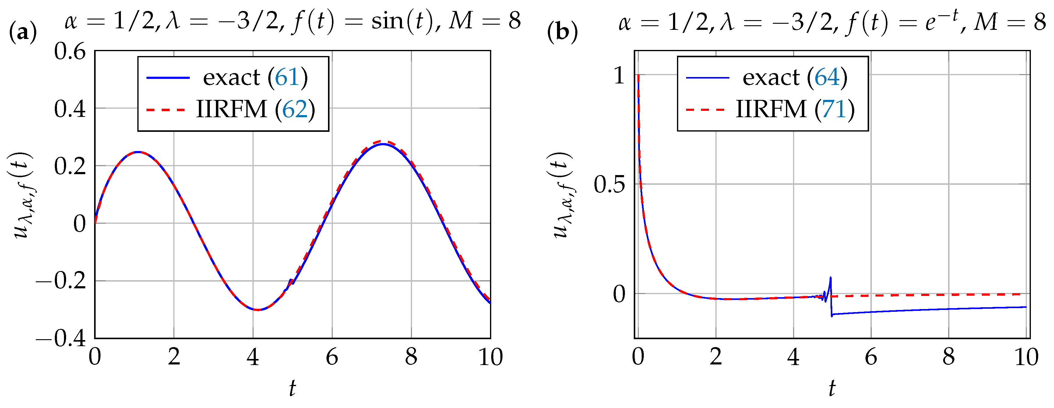
Sinusoidal Source Term $f\left(t\right)=sin\left(t\right)$

This is another source term that ensures a zero initial condition. An analytical expression $u_{\lambda ,{\displaystyle \frac{1}{2}},f}\left(t\right)$ of the solution also exists here:

$$\begin{array}{cc}\hfill u_{\lambda ,{\displaystyle \frac{1}{2}},f}\left(t\right)& ={\displaystyle \frac{\pi {\lambda }^2{e}^{\pi {\lambda }^{2}t}{g}_{\lambda }\left(t\right)}{{\pi }^2{\lambda }^4+1}}+{\displaystyle \frac{\sqrt{2\pi }\lambda \mathrm{FS}\left(\sqrt{\frac{2}{\pi }t}\right)\left[\pi {\lambda }^{2}sin\left(t\right)+cos\left(t\right)\right]}{{\pi }^2{\lambda }^4+1}}\hfill \\ \hfill & -{\displaystyle \frac{\left[\sqrt{2\pi }\lambda \mathrm{FC}\left(\sqrt{\frac{2}{\pi }t}\right)+1\right]\left[\pi {\lambda }^{2}cos\left(t\right)-sin\left(t\right)\right]}{{\pi }^2{\lambda }^4+1}},\hfill \end{array}$$

(61)

where FC and FS are the Fresnel integrals, defined by $\mathrm{FS}\left(x\right)={\int }_0^{x}sin\left(\pi t^2/2\right)\mathrm{d}t$ and $\mathrm{FC}\left(x\right)={\int }_0^{x}cos\left(\pi t^2/2\right)\mathrm{d}t$. The $g_{\lambda }\left(t\right)$ function with pathological numerical behavior in single precision is again found here. It has also been possible to determine here an explicit expression for the IIRFM numerical solution, as follows:

$$u_{\lambda ,{\displaystyle \frac{1}{2}},f}^{\mathrm{IIR},M}\left(t_k\right)=sin\left(t_k\right)+2cos\left({\displaystyle \frac{T_e}{2}}\right)F_{M,T_e}\left(t_k\right),$$

(62)

with $F_{M,T_e}\left(t_k\right)$ given by

$$F_{M,T_e}\left(t_k\right)=\sum _{i=1}^M{A}_{M,i}{\displaystyle \frac{\left(B_{M,i}+1\right)B_{M,i}^{t_k/T_e}sin\left(\frac{T_e}{2}\right)-B_{M,i}sin\left(t_k+\frac{T_e}{2}\right)+sin\left(t_k-\frac{T_e}{2}\right)}{{\left[B_{M,i}-cos\left(T_e\right)\right]}^2+{sin}^2\left(T_e\right)}},$$

(63)

where $A_{M,i}$ and $B_{M,i}$ have the same expressions as in previous examples.

Figure 10a compares the plots obtained using analytical (61) and numerical IIRFM (62) solutions. The problem of artificial discontinuities in the graphical representation of the analytical solution, due to the presence of the function $g_{\lambda }\left(t\right)$ in (61), is very pronounced here in the vicinity of $t\approx 5$. These defects are not present in the plot obtained by the IIRFM (dashed line), which here gives better numerical results in single precision than using the analytical expression.

Figure 10. (a) Analytical solution (61) and numerical IIRFM solution (62) when $f\left(t\right)=sin\left(t\right)$, $\alpha =1/2$, $\lambda =-3/2$, $M=8$, and $T_e=0.05$. (b) Analytical solution (64) and numerical IIRFM solution (71) when $f\left(t\right)=e^{-t}$, $\alpha =1/2$, $\lambda =-3/2$, $M=8$, and $T_e=0.05$.

Exponential Source Term $f\left(t\right)=e^{-t}$

For this last example, the case of a non-zero initial condition is considered, since here $u_{\lambda ,{\displaystyle \frac{1}{2}},f}\left(0\right)=f\left(0\right)=1$. Using Equation (4), it is possible to find an analytical solution to the problem (3) when $f\left(t\right)=e^{-t}$ and $\alpha =1/2$, whose expression is as follows:

$$u_{\lambda ,{\displaystyle \frac{1}{2}},e^{-t}}\left(t\right)=2\lambda \mathrm{DF}\left(\sqrt{t}\right)+{\displaystyle \frac{\pi {\lambda }^2{e}^{\pi {\lambda }^{2}t}{g}_{\lambda }\left(t\right)+e^{-t}\left[1-{\pi }^{3/2}{\lambda }^3\mathrm{erfi}\left(\sqrt{t}\right)\right]}{1+\pi {\lambda }^2}},$$

(64)

where $\mathrm{DF}\left(x\right)=e^{-x^2}{\int }_0^x{e}^{y^2}\mathrm{d}y$ is the Dawson function and $\mathrm{erfi}\left(x\right)=\mathrm{erf}\left(\mathrm{i}x\right)/\mathrm{i}$ is the imaginary error function, with ${\mathrm{i}}^2=-1$. The presence of the function $g_{\lambda }\left(t\right)$ in the analytical expression of the solution leads, as shown in Figure 10b, to considerable difficulties in graphically representing the function $u_{\lambda ,{\displaystyle \frac{1}{2}},e^{-t}}\left(t\right)$ given by Equation (64) in single precision.

When $\alpha \ne 0$, applying the IIRFM to numerically solve Equation (3) assumes the initial condition on the solution to be null. If $\alpha \ne 0$ and the initial condition is non-zero but finite, then we introduce the auxiliary functions $v_{\lambda ,\alpha ,f_0}\left(t\right)$ and $w_{\lambda ,\alpha ,f\left(0\right)}\left(t\right)$, which satisfy the following auxiliary integral equations:

$$\left|\begin{array}{c}{v}_{\lambda ,\alpha ,f_0}\left(t\right)=f_0\left(t\right)+\lambda {\int }_0^t{\displaystyle \frac{v_{\lambda ,\alpha ,f_0}\left(t^{\prime }\right)}{{(t-t^{\prime })}^{\alpha }}}\mathrm{d}{t}^{\prime },\hfill \\ w_{\lambda ,\alpha ,f\left(0\right)}\left(t\right)=f\left(0\right)+\lambda {\int }_0^t{\displaystyle \frac{w_{\lambda ,\alpha ,f\left(0\right)}\left(t^{\prime }\right)}{{(t-t^{\prime })}^{\alpha }}}\mathrm{d}{t}^{\prime },\hfill \end{array}\right.$$

(65)

with $f_0\left(t\right)=f\left(t\right)-f\left(0\right)$. The $u_{\lambda ,\alpha ,f}\left(t\right)$ solution sought is written as $u_{\lambda ,\alpha ,f}\left(t\right)=v_{\lambda ,\alpha ,f_0}\left(t\right)+w_{\lambda ,\alpha ,f\left(0\right)}\left(t\right)$, which satisfies Equation (3), with the initial condition $u_{\lambda ,\alpha ,f}\left(0\right)=f\left(0\right)$. Two important special cases should be noted: firstly, in the case where $f\left(0\right)=0$, the result is $w_{\lambda ,\alpha ,f\left(0\right)}\left(t\right)=0$, and the situation with zero initial condition studied in the previous paragraphs is retrieved. On the other hand, when $f\left(t\right)=C=\mathrm{cste}$, in this case $f_0\left(t\right)=0$ results in $v_{\lambda ,\alpha ,f_0}\left(t\right)=0$.

The calculation of $v_{\lambda ,\alpha ,f_0}\left(t\right)$ by the IIRFM has already been described in previous paragraphs, with $f_0\left(0\right)=0\Rightarrow v_{\lambda ,\alpha ,f_0}\left(0\right)=0$. General result (24) is still applicable and it is also possible to find here an explicit expression of the IIRFM numerical solution for $f\left(t\right)=e^{-t}\Rightarrow f_0\left(t\right)=e^{-t}-1$, which holds for $\alpha =1/2$, as follows:

$$\begin{array}{cc}\hfill v_{\lambda ,{\displaystyle \frac{1}{2}},f_0}^{\mathrm{IIR},M}\left(t_k\right)& =e^{-t_k}-1\hfill \\ \hfill & +\sum _{i=1}^M{A}_{M,i}{\displaystyle \frac{\left(1-B_{M,i}\right)\left(1+e^{T_e}\right)e^{-t_k}-2\left(1-e^{T_e}{B}_{M,i}\right)+B_{M,i}^{t_k/T_e}\left(1+B_{M,i}\right)\left(1-e^{T_e}\right)}{\left(1-B_{M,i}\right)\left(1-e^{T_e}{B}_{M,i}\right)}}.\hfill \end{array}$$

(66)

There remains the need to explain the calculation of $w_{\lambda ,\alpha ,f\left(0\right)}\left(t\right)$. Since the source term $f\left(0\right)$ is constant here, the auxiliary solution $w_{\lambda ,\alpha ,f\left(0\right)}\left(t\right)$ can always be written as $w_{\lambda ,\alpha ,f\left(0\right)}\left(t\right)=f\left(0\right)w_{\lambda ,\alpha }^0\left(t\right)$, where the function $w_{\lambda ,\alpha }^0\left(t\right)$ is independent of the expression of the source term $f\left(t\right)$ considered in the integral Equation (3). This means that there is only one possible function $w_{\lambda ,\alpha }^0\left(t\right)$ for a given set of parameters $(\alpha ,\lambda )$. More precisely, the function $w_{\lambda ,\alpha }^0\left(t\right)$ is given by the following inverse Laplace transform:

$$w_{\lambda ,\alpha }^0\left(t\right)={\mathcal{L}}^{-1}\left[{\displaystyle \frac{1}{s-\lambda \Gamma \left(1-\alpha \right)s^{\alpha }}}\right].$$

(67)

Depending on the value taken by $\alpha$, different approaches can be adopted to calculate $w_{\lambda ,\alpha }^0\left(t\right)$. In the case of the present paragraph where $\alpha =1/2$, the inverse Laplace transform (67) can be computed explicitly and leads to the following analytical expression of $w_{\lambda ,{\displaystyle \frac{1}{2}}}^0\left(t\right)$:

$$w_{\lambda ,{\displaystyle \frac{1}{2}}}^0\left(t\right)=e^{{\lambda }^2\pi t}\left[1+\mathrm{erf}\left(\lambda \sqrt{\pi t}\right)\right]=e^{\pi {\lambda }^{2}t}{g}_{\lambda }\left(t\right).$$

(68)

Finally, the IIRFM solution of the initial problem is written here for $f\left(t\right)=e^{-t}$ and $\alpha =1/2$:

$$u_{\lambda ,{\displaystyle \frac{1}{2}},e^{-t}}^{\mathrm{IIR},M}\left(t_k\right)=v_{\lambda ,{\displaystyle \frac{1}{2}},f_0}^{\mathrm{IIR},M}\left(t_k\right)+f\left(0\right)e^{\pi {\lambda }^2{t}_k}{g}_{\lambda }\left(t_k\right),$$

(69)

where $v_{\lambda ,{\displaystyle \frac{1}{2}},f_0}^{\mathrm{IIR},M}$ is given by (66). This expression of $u_{\lambda ,{\displaystyle \frac{1}{2}},e^{-t}}^{\mathrm{IIR},M}$ involves the function $g_{\lambda }\left(t\right)$, whose anomalous numerical behavior in single precision has been highlighted in the previous paragraphs for $\lambda \sqrt{\pi t}\lesssim -5$. Equation (69) is therefore acceptable as long as $0⩽t⩽{\displaystyle \frac{1}{\pi }}{\left({\displaystyle \frac{5}{\lambda }}\right)}^2$. When $t>{\displaystyle \frac{1}{\pi }}{\left({\displaystyle \frac{5}{\lambda }}\right)}^2$, we recommend not using the analytical expression of the function $g_{\lambda }\left(t\right)$, but rather resorting to the following numerical form:

$$u_{\lambda ,{\displaystyle \frac{1}{2}},e^{-t}}^{\mathrm{IIR},M}\left(t_k\right)=v_{\lambda ,{\displaystyle \frac{1}{2}},f_0}^{\mathrm{IIR},M}\left(t_k\right)+f\left(0\right)e^{\pi {\lambda }^2{t}_k}{g}_{\lambda }^{\mathrm{IIR},M}\left(t_k\right).$$

(70)

Result (60) finally allows to write $u_{\lambda ,{\displaystyle \frac{1}{2}},e^{-t}}^{\mathrm{IIR},M}\left(t_k\right)$ in a fully numerical form:

$$u_{\lambda ,{\displaystyle \frac{1}{2}},e^{-t}}^{\mathrm{IIR},M}\left(t_k\right)=v_{\lambda ,{\displaystyle \frac{1}{2}},f_0}^{\mathrm{IIR},M}\left(t_k\right)+f\left(0\right)\left[\pi {\lambda }^2{u}_{\lambda ,{\displaystyle \frac{1}{2}},t}^{\mathrm{IIR},M}\left(t_k\right)+1+2\lambda \sqrt{t_k}\right],$$

(71)

where $v_{\lambda ,{\displaystyle \frac{1}{2}},f_0}^{\mathrm{IIR},M}\left(t_k\right)$ is given by (66) and $u_{\lambda ,{\displaystyle \frac{1}{2}},t}^{\mathrm{IIR},M}\left(t_k\right)$ is given by (58). This result is particularly interesting, since it holds (for the Abelian kernel $\alpha =1/2$) whatever the value of $\lambda ⩽0$ and whatever the expression of $f\left(t\right)$, provided that $f\left(0\right)$ is finite. Note that this result does not involve any numerical inversion of Laplace transforms, and that it generalizes the IIRFM for solving Abel integral equations of the second kind for $\alpha =1/2$, to the case of non-zero but finite initial conditions.

Constant Term Source $f\left(t\right)=C$

In the present case, we consider $f_0\left(t\right)=f\left(t\right)-f\left(0\right)=0$ and $f\left(0\right)=C$, leading to the following expressions for the auxiliary functions $v_{\lambda ,\alpha ,f_0}\left(t\right)$ and $w_{\lambda ,\alpha ,f\left(0\right)}\left(t\right)$:

$$\left|\begin{array}{c}{v}_{\lambda ,\alpha ,f_0}\left(t\right)=\lambda {\int }_0^t{\displaystyle \frac{v_{\lambda ,\alpha ,f_0}\left(t^{\prime }\right)}{{(t-t^{\prime })}^{\alpha }}}\mathrm{d}{t}^{\prime }=0,\hfill \\ w_{\lambda ,\alpha ,f\left(0\right)}\left(t\right)=C+\lambda {\int }_0^t{\displaystyle \frac{w_{\lambda ,\alpha ,f\left(0\right)}\left(t^{\prime }\right)}{{(t-t^{\prime })}^{\alpha }}}\mathrm{d}{t}^{\prime }.\hfill \end{array}\right.$$

(72)

The analytical solution of the problem is deduced from the developments of Section “Exponential Source Term $f\left(t\right)=e^{-t}$”:

$$u_{\lambda ,{\displaystyle \frac{1}{2}},C}\left(t\right)=e^{\pi {\lambda }^{2}t}\left[1+\mathrm{erf}\left(\lambda \sqrt{\pi t}\right)\right].$$

(73)

The expression for the IIRFM solution is deduced from Section “Exponential Source Term $f\left(t\right)=e^{-t}$” for the present case, as follows:

$$u_{\lambda ,{\displaystyle \frac{1}{2}},C}^{\mathrm{IIR},M}\left(t_k\right)=C\left[\pi {\lambda }^2{u}_{\lambda ,{\displaystyle \frac{1}{2}},t}^{\mathrm{IIR},M}\left(t_k\right)+1+2\lambda \sqrt{t_k}\right].$$

(74)

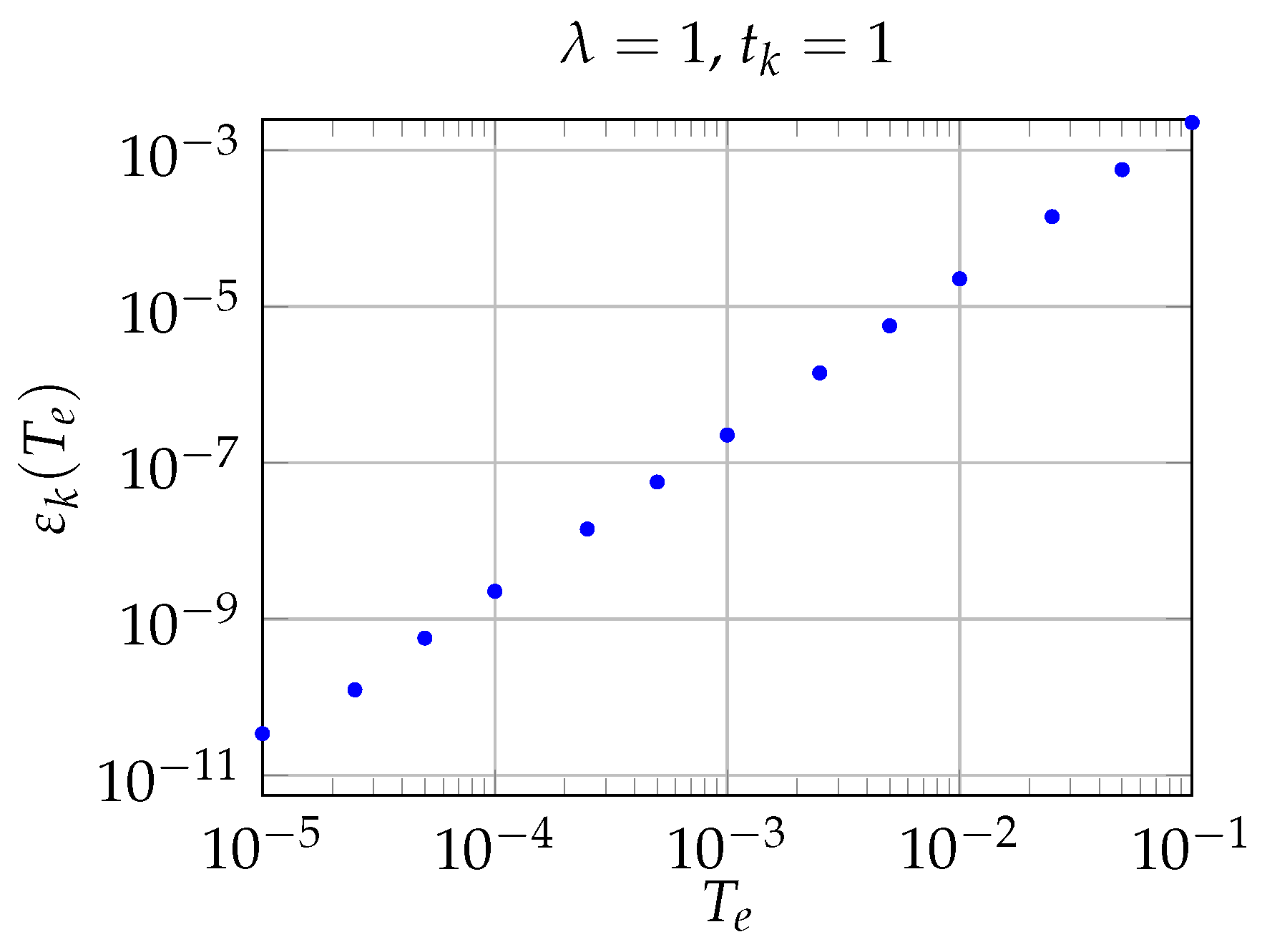
3.2.2. IIRFM Approach When $\alpha =1/2$ and $\lambda >0$

When $\lambda >0$, the denominator of the Laplace transfer function $H_{\alpha }(s,\lambda )$ admits a positive root $s_{\lambda }$, whose expression is $s_{\lambda }=\lambda \Gamma {(1-\alpha )}^{1/(1-\alpha )}$. The transfer function $H_{\mathrm{L},\alpha }(s,\lambda )$ in this case presents a singularity at $s=s_{\lambda }$. To allow a precise determination of the coefficients $a_{M,i}$ and $b_{M,i}$ of Equation (18), despite the singularity at $s_{\lambda }$, we first calculate a Chebyshev rational interpolation (denoted by ${\mathrm{RF}}_c^M$) of the function $(s-s_{\lambda })\times \left[H_{\mathrm{L},\alpha }(s,\lambda )-1\right]$. This interpolation is written as

$${\mathrm{RF}}_c^M\left\{(s-s_{\lambda })\times \left[H_{\mathrm{L},\alpha }(s,\lambda )-1\right]\right\}={\displaystyle \frac{{\sum }_{i=0}^{M-1}{a}_{M,i}^{\prime }\left(\alpha ,\lambda \right)s^i}{1+{\sum }_{i=1}^{M-1}{b}_{M,i}^{\prime }\left(\alpha ,\lambda \right)s^i}}.$$

(75)

The following approximate form $H_{\mathrm{L},\alpha }^M(s,\lambda )$ of the transfer function $H_{\mathrm{L},\alpha }(s,\lambda )$ is deduced:

$$H_{\mathrm{L},\alpha }^M(s,\lambda )=1+{\displaystyle \frac{{\sum }_{i=0}^{M-1}{a}_{M,i}^{\prime }\left(\alpha ,\lambda \right)s^i}{{\sum }_{i=0}^M{b}_{M,i}^{\prime \prime }\left(\alpha ,\lambda \right)s^i}},$$

(76)

with $b_{M,0}^{\prime \prime }=-s_{\lambda }$, $b_{M,1}^{\prime \prime }=1-b_{M,1}^{\prime }{s}_{\lambda }$, $b_{M,M}^{\prime \prime }=b_{M,M-1}^{\prime }$ and $b_{M,m}^{\prime \prime }=b_{M,m-1}^{\prime }-b_{M,m}^{\prime }{s}_{\lambda }$ for $m\in [2,M-1]$. Further developments are strictly identical to those exposed in the previous paragraphs for $\lambda <0$ and will therefore not be repeated here. Note also that all the results established in Section “Exponential Source Term $f\left(t\right)=e^{-t}$” remain applicable here, but with $\lambda >0$.

As an example, let us consider the case where $f\left(t\right)=e^{-t}$, $\alpha =\lambda =1/2$, for which it is found that $s_{\lambda }\approx 0.7853982$. The rational approximation (75) has in this case been calculated over the interpolation interval $I_s=[s_{\lambda },5s_{\lambda }]$, for $M=4$. Figure 11a shows the analytical (64) and numerical IIRFM (71) solutions in the present case, for $t\in [0,3]$ and $T_e=5\times {10}^{-3}$. Figure 11b shows the relative error ${\epsilon }_r=100\times (u_{{\displaystyle \frac{1}{2}},{\displaystyle \frac{1}{2}},e^{-t}}^{\mathrm{IIR},4}/u_{{\displaystyle \frac{1}{2}},{\displaystyle \frac{1}{2}},e^{-t}}-1)$ in %, as a function of t. The correspondence between analytical and IIRFM resolutions is excellent, even for the low M value considered here.

Figure 11. IIRFM solution of Equation (3), for $\lambda =\alpha =1/2$, $f\left(t\right)=e^{-t}$, $T_e=5\times {10}^{-3}$, and $M=4$. (a) Changes in analytical and numerical solutions as a function of t. (b) Relative error ${\epsilon }_r=100\times (u_{{\displaystyle \frac{1}{2}},{\displaystyle \frac{1}{2}},e^{-t}}^{\mathrm{IIR},4}/u_{{\displaystyle \frac{1}{2}},{\displaystyle \frac{1}{2}},e^{-t}}-1)$ in %.

3.2.3. Comparison of the IIRFM with the Mouley et al. [13] Approach

In this section, the IIRFM is applied to the numerical solution of two second-kind Abel linear integral equations, which Mouley et al. have studied using a recent numerical method based on an approximation involving Daubechies wavelets [13]. The accuracy of the results provided by the two methods is compared on two examples, for different orders of approximation (see Table 4 and Table 5).

First Example

Consider the following Abel integral equation of the second kind (there is a typographical error in the paper by Mouley et al. where ${\displaystyle \frac{16}{5}}{t}^{5/2}$ is found in place of ${\displaystyle \frac{16}{15}}{t}^{5/2}$):

$$u\left(t\right)=t^2+{\displaystyle \frac{16}{15}}{t}^{{\displaystyle \frac{5}{2}}}-{\int }_0^t{\displaystyle \frac{u\left(t^{\prime }\right)}{\sqrt{t-t^{\prime }}}}\mathrm{d}{t}^{\prime },$$

(77)

which admits as analytical solution the function $u\left(t\right)=t^2$. This is a convolutive integral equation of the form (3), with $\alpha =1/2$, $\lambda =-1$, $f\left(t\right)=t^2+{\displaystyle \frac{16}{15}}{t}^{5/2}$, and $u\left(0\right)=0$. The developments of Section 3.2.1 are therefore directly applicable to the numerical solution of this integral equation using the IIRFM method.

Table 4 gathers the absolute errors ${\epsilon }_{\mathrm{Dau}}^j=\left|u\left(t\right)-u_{\mathrm{Dau}}^j\left(t\right)\right|$ committed using the Mouley et al. method and absolute errors ${\epsilon }_{\mathrm{IIR}}^M=\left|u\left(t\right)-u_{\mathrm{IIR}}^M\left(t\right)\right|$ committed using the IIRFM (with $I_s=[0,15]$ and $T_e={10}^{-3}$), for different values of $t\in [0,1]$, different resolutions j, and for different approximation orders M.

Table 4. Absolute errors in the numerical resolution of (77) using the Mouley et al. [13] and IIRFM methods (with $I_s=[0,15]$ and $T_e={10}^{-3}$).

		${\mathit{\epsilon }}_{\mathbf{Dau}}^{\mathit{j}}\times {10}^6$			${\mathit{\epsilon }}_{\mathbf{IIR}}^{\mathit{M}}\times {10}^6$
$\mathit{t}$	Exact Values	$\mathit{j}=\mathbf{4}$	$\mathit{j}=\mathbf{6}$	$\mathit{j}=\mathbf{8}$	$\mathit{M}=\mathbf{4}$	$\mathit{M}=\mathbf{6}$	$\mathit{M}=\mathbf{8}$
$0.125$	$0.015625$	117	1	0	1	0	0
$0.25$	$0.062500$	37	1	0	2	0	0
$0.375$	$0.140625$	22	0	0	12	0	0
$0.5$	$0.250000$	16	0	0	3	1	0
$0.625$	$0.390625$	12	0	0	23	1	0
$0.75$	$0.562500$	10	0	0	37	1	0
$0.875$	$0.765625$	8	0	0	21	1	0

Table 4. Absolute errors in the numerical resolution of (77) using the Mouley et al. [13] and IIRFM methods (with $I_s=[0,15]$ and $T_e={10}^{-3}$).

		${\mathit{\epsilon }}_{\mathbf{Dau}}^{\mathit{j}}\times {10}^6$			${\mathit{\epsilon }}_{\mathbf{IIR}}^{\mathit{M}}\times {10}^6$
$\mathit{t}$	Exact Values	$\mathit{j}=\mathbf{4}$	$\mathit{j}=\mathbf{6}$	$\mathit{j}=\mathbf{8}$	$\mathit{M}=\mathbf{4}$	$\mathit{M}=\mathbf{6}$	$\mathit{M}=\mathbf{8}$
$0.125$	$0.015625$	117	1	0	1	0	0
$0.25$	$0.062500$	37	1	0	2	0	0
$0.375$	$0.140625$	22	0	0	12	0	0
$0.5$	$0.250000$	16	0	0	3	1	0
$0.625$	$0.390625$	12	0	0	23	1	0
$0.75$	$0.562500$	10	0	0	37	1	0
$0.875$	$0.765625$	8	0	0	21	1	0

It can be seen from these results that the accuracies obtained with the IIRFM are, in the case of integral Equation (77), quite comparable with those provided by the method of Mouley et al. [13].

Second Example

Let us now consider the following Abel integral equation of the second kind, also studied by Mouley et al. in [13]:

$$u\left(t\right)={\displaystyle \frac{1}{\sqrt{t+1}}}+{\displaystyle \frac{\pi }{8}}-{\displaystyle \frac{1}{4}}{sin}^{-1}\left({\displaystyle \frac{1-t}{1+t}}\right)-{\displaystyle \frac{1}{4}}{\int }_0^t{\displaystyle \frac{u\left(t^{\prime }\right)}{\sqrt{t-t^{\prime }}}}\mathrm{d}{t}^{\prime },$$

(78)

of which the analytical solution is $u\left(t\right)=1/\sqrt{t+1}$. This is still a convolutive integral equation of the form (3), with $\alpha =1/2$, $\lambda =-1/4$, $f\left(t\right)=1/\sqrt{t+1}+{\displaystyle \frac{\pi }{8}}-{\displaystyle \frac{1}{4}}{sin}^{-1}\left({\displaystyle \frac{1-t}{1+t}}\right)$, and $u\left(0\right)=1$.

Table 5 gathers the absolute errors ${\epsilon }_{\mathrm{Dau}}^j$ and ${\epsilon }_{\mathrm{IIR}}^M$ committed by numerically calculating the solution of (78), for different values of $t\in [0,1]$, for different resolutions j, and different approximation orders M.

Table 5. Absolute errors $\epsilon$ in the numerical resolution of (78) using the Mouley et al. [13] and IIRFM methods (with $I_s=[0,15]$ and $T_e={10}^{-3}$).

		${\mathit{\epsilon }}_{\mathbf{Dau}}^{\mathit{j}}\times {10}^6$			${\mathit{\epsilon }}_{\mathbf{IIR}}^{\mathit{M}}\times {10}^6$
$\mathit{t}$	$\mathbf{1}/\sqrt{\mathit{t}+\mathbf{1}}$	$\mathit{j}=\mathbf{4}$	$\mathit{j}=\mathbf{6}$	$\mathit{j}=\mathbf{8}$	$\mathit{M}=\mathbf{4}$	$\mathit{M}=\mathbf{6}$	$\mathit{M}=\mathbf{8}$
$0.125$	$0.942809$	21,732	4370	1074	29	3	3
$0.25$	$0.894427$	10,739	2774	683	28	3	1
$0.375$	$0.852803$	8568	2091	515	15	1	1
$0.5$	$0.816497$	6971	1695	417	32	1	1
$0.625$	$0.784465$	5890	1433	353	9	2	1
$0.75$	$0.755929$	5113	1244	307	27	1	1
$0.875$	$0.730297$	4522	1101	271	54	1	0

Table 5. Absolute errors $\epsilon$ in the numerical resolution of (78) using the Mouley et al. [13] and IIRFM methods (with $I_s=[0,15]$ and $T_e={10}^{-3}$).

		${\mathit{\epsilon }}_{\mathbf{Dau}}^{\mathit{j}}\times {10}^6$			${\mathit{\epsilon }}_{\mathbf{IIR}}^{\mathit{M}}\times {10}^6$
$\mathit{t}$	$\mathbf{1}/\sqrt{\mathit{t}+\mathbf{1}}$	$\mathit{j}=\mathbf{4}$	$\mathit{j}=\mathbf{6}$	$\mathit{j}=\mathbf{8}$	$\mathit{M}=\mathbf{4}$	$\mathit{M}=\mathbf{6}$	$\mathit{M}=\mathbf{8}$
$0.125$	$0.942809$	21,732	4370	1074	29	3	3
$0.25$	$0.894427$	10,739	2774	683	28	3	1
$0.375$	$0.852803$	8568	2091	515	15	1	1
$0.5$	$0.816497$	6971	1695	417	32	1	1
$0.625$	$0.784465$	5890	1433	353	9	2	1
$0.75$	$0.755929$	5113	1244	307	27	1	1
$0.875$	$0.730297$	4522	1101	271	54	1	0

This time, it was found that the accuracy of the numerical resolution of (78) by the IIRFM (with $I_s=[0,15]$ and $T_e={10}^{-3}$) is much better than the accuracy allowed by the method of Mouley et al., which uses Daubechy wavelets. Despite the greater complexity of the source function $f\left(t\right)$ considered in this second example, the accuracy obtained here with the IIRFM remains comparable to that obtained with the same method for the previous example. This is a clear advantage of the IIRFM in the present case, as it is found that the accuracy depends relatively little on the complexity of the source function $f\left(t\right)$.

3.2.4. Comparison of the IIRFM with the Singha et al.  [14] Approach

In the present section, the results obtained with the IIRFM are compared with the numerical results obtained using Laguerre polynomials $L_i$ of order i [14], at approximation order $M=5$:

$$u_S^M\left(t\right)=\sum _{i=0}^M{\ell }_i{L}_i\left(t\right),$$

(79)

where $u_S^M\left(t\right)$ is the approximation of Singha et al.

The accuracy of the results provided by the two methods is compared in two examples proposed by Singha et al. in [14].

First Example

Consider the following Abel integral equation of the second kind:

$$u\left(t\right)={\displaystyle \frac{\pi t}{2}}+\sqrt{t}-{\int }_0^t{\displaystyle \frac{u\left(t^{\prime }\right)}{\sqrt{t-t^{\prime }}}}\mathrm{d}{t}^{\prime },$$

(80)

of which analytical solution is $u\left(t\right)=\sqrt{t}$. This is a convolutive integral equation of the form (3), with $\alpha =1/2$, $\lambda =-1$, $f\left(t\right)={\displaystyle \frac{\pi t}{2}}+\sqrt{t}$, and $u\left(0\right)=0$. Table 6 gathers the absolute errors $\epsilon$ committed by numerically calculating the solution of (80), with the polynomial method proposed by Singha et al. [14] and with the IIRFM, for different values of $t\in [0,2]$, and for the same order of approximation $M=5$.

Table 6. Absolute errors $\epsilon$ in the numerical resolution of (80) by the Laguerre approximation (Singha et al. [14]) and by the IIRFM (with $I_s=[0,15]$ and $T_e={10}^{-3}$), and for the same order of approximation $M=5$.

		Approximated Solutions		Absolute Errors: $\mathit{\epsilon }\times {10}^6$
$\mathit{t}$	$\sqrt{\mathit{t}}$	Laguerre	IIRFM	Laguerre	IIRFM
$0.2$	$0.44721360$	$0.42222142$	$0.44717924$	24,992	34
$0.4$	$0.63245553$	$0.60061467$	$0.63247236$	31,841	17
$0.6$	$0.77459667$	$0.75640000$	$0.77454516$	18,197	52
$0.8$	$0.89442719$	$0.89246899$	$0.89446429$	1958	37
$1.0$	$1.00000000$	$1.01148725$	$1.00009060$	11,487	91
$2.0$	$1.41421356$	$1.42927171$	$1.41397446$	15,058	239

The results in Table 6 clearly demonstrate the benefits of the IIRFM for the numerical resolution of (80). For each value of t considered, the IIRFM is always much more accurate here than the approach proposed by Singha et al. [14].

The values of the Laguerre approximation $u_S^M\left(t\right)={\sum }_{i=0}^M{\ell }_i{L}_i\left(t\right)$ have been calculated here using the $\left\{{\ell }_i\right\}$ coefficient values of Singha et al. [14]:

$$\{{\ell }_0,{\ell }_1,{\ell }_2,{\ell }_3,{\ell }_4,{\ell }_5\}=\sqrt{\pi }\times \left\{{\displaystyle \frac{1}{2}},-{\displaystyle \frac{1}{4}},-{\displaystyle \frac{1}{16}},-{\displaystyle \frac{1}{32}},-{\displaystyle \frac{5}{256}},-{\displaystyle \frac{7}{512}}\right\}.$$

(81)

Second Example

Consider the following Abel integral equation of the second kind:

$$u\left(t\right)=\sqrt{\pi }{\displaystyle \frac{\Gamma \left(\frac{5}{4}\right)}{\Gamma \left(\frac{7}{4}\right)}}{t}^{{\displaystyle \frac{3}{4}}}+t^{{\displaystyle \frac{1}{4}}}-{\int }_0^t{\displaystyle \frac{u\left(t^{\prime }\right)}{\sqrt{t-t^{\prime }}}}\mathrm{d}{t}^{\prime },$$

(82)

which admits the analytical solution $u\left(t\right)=t^{1/4}$. This is a convolutive integral equation of the form (3), with $\alpha =1/2$, $\lambda =-1$, $f\left(t\right)=\sqrt{\pi }{\displaystyle \frac{\Gamma \left(\frac{5}{4}\right)}{\Gamma \left(\frac{7}{4}\right)}}{t}^{{\displaystyle \frac{3}{4}}}+t^{{\displaystyle \frac{1}{4}}}$ and $u\left(0\right)=0$. Table 7 gathers the absolute errors $\epsilon$ committed by numerically calculating the solution of (78) with the polynomial method of Singha et al. [14] and with the IIRFM, for different values of $t\in [0,2]$, and for the same order of approximation $M=5$.

Table 7. Absolute errors $\epsilon$ in the numerical resolution of (82) by the Laguerre approximation (Singha et al. [14]) and by the IIRFM (with $I_s=[0,15]$ and $T_e={10}^{-3}$), and for the same order of approximation $M=5$.

		Approximated Solutions		Absolute Errors: $\mathit{\epsilon }\times {10}^6$
$\mathit{t}$	${\mathit{t}}^{\mathbf{1}/\mathbf{4}}$	Laguerre	IIRFM	Laguerre	IIRFM
$0.2$	$0.66874030$	$0.63419588$	$0.66876039$	34,544	20
$0.4$	$0.79527073$	$0.75840545$	$0.79527721$	38,653	6
$0.6$	$0.88011174$	$0.86140153$	$0.88004956$	18,710	62
$0.8$	$0.94574161$	$0.94609498$	$0.94584299$	353	101
$1.0$	$1.00000000$	$1.01516222$	$1.00013177$	15,162	132
$2.0$	$1.18920712$	$1.20439817$	$1.18901343$	15,191	194

It can also be seen here that the numerical resolution of Equation (82) by the IIRFM remains overall more accurate than the resolution made with the numerical method of Singha et al., and for which the absolute error suffers significant variations over the range of t values studied.

The values of the Laguerre approximation $u_S^M\left(t\right)={\sum }_{i=0}^M{\ell }_i{L}_i\left(t\right)$ have been calculated here using the $\left\{{\ell }_i\right\}$ coefficient values of Singha et al. [14]:

$$\{{\ell }_0,{\ell }_1,{\ell }_2,{\ell }_3,{\ell }_4,{\ell }_5\}=\left\{0.906402,-0.226601,-0.084975,-0.049569,-0.0340787,-0.025559\right\}$$

(83)

3.3. Logarithmic Kernel

We now consider the case of a logarithmic kernel $K(t,t^{\prime })=ln\left(\left|t-t^{\prime }\right|\right)$, for which $\overline{K}\left(s\right)=-[\gamma +ln\left(s\right)]/s$. The Laplace transfer function $H_{\mathrm{L}}(s,\lambda )$ associated with Equation (2) becomes

$$H_{\mathrm{L}}(s,\lambda )={\displaystyle \frac{1}{1+\lambda \left[\gamma +ln\left(s\right)\right]/s}},$$

(84)

where $\gamma \approx 0.577216$ is the Euler constant. The transfer function $H_{\mathrm{L}}(s,\lambda )$ in this case admits a pole $s_{\lambda }$, which is the root of the non linear equation $e^{-\gamma }=s{e}^{s/\lambda }$, given by the Lambert W function: $s_{\lambda }=\lambda W\left(e^{-\gamma }/\lambda \right)$. The same process is used here as in Section 3.2.2, for which it is recalled that the first step consists of calculating a rational Chebyshev interpolation (noted ${\mathrm{RF}}_c^M$) of the function $(s-s_{\lambda })\times \left[H(s,\lambda )-1\right]$.

In the following paragraphs, two examples of IIRFM solving Equation (2) with logarithmic kernel are presented when $\lambda =1$. Refer to Section 3.2.1 and Section 3.2.2 for details of the different steps involved in implementing the IIRFM in the present case.

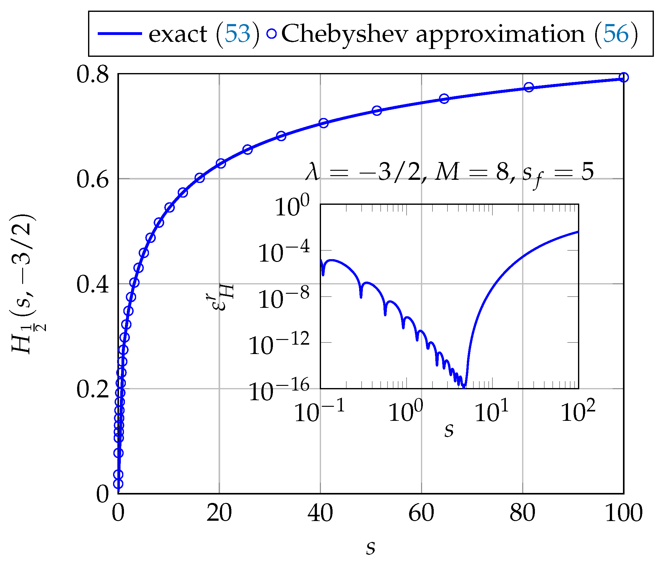
3.3.1. First Example: $f\left(t\right)=t+{\displaystyle \frac{1}{4}}{t}^2[3-2ln\left(t\right)]$

Equation (2) admits in the present case the following analytical solution $u_{1,f}\left(t\right)=t$, with zero initial condition.

Figure 12 compares the numerical results obtained with the IIRFM (for an order of approximation $M=5$) with the results obtained with the analytical solution. The relative error shown in Figure 12b here remains quite small, especially for increasing values of t, attesting to the stability of the IIRFM in this case, despite the presence of a pole in the transfer function $H_{\mathrm{L}}(s,\lambda )$.

Figure 12. IIRFM resolution of Equation (2) considering a logarithmic kernel, with $\lambda =1$, $f\left(t\right)=t+{\displaystyle \frac{1}{4}}{t}^2[3-2ln\left(t\right)]$, $T_e={10}^{-2}$, $M=5$, and an interpolation interval $I_s=[s_{\lambda },5s_{\lambda }]$. (a) Changes in the analytical and numerical solutions as a function of t. (b) Relative error ${\epsilon }_r=100\times (u_{1,f}^{\mathrm{IIR},5}/u_{1,f}-1)$ in %.

3.3.2. Second Example: $f\left(t\right)=1-e^{-t/\tau }+\lambda \left[t+(\tau -t)ln\left(t\right)\right]+$ $\lambda \tau e^{-t/\tau }\left(\gamma -ln\left(\tau \right)+\mathrm{i}\pi +{\int }_{-t/\tau }^{\infty }{\displaystyle \frac{e^{-x}}{x}}\mathrm{d}x\right)$

Equation (2) admits in the present case the following analytical solution $u_{1,f}\left(t\right)=1-e^{-t/\tau }$. Figure 12 compares the numerical results obtained with the IIRFM (for an order of approximation $M=5$) with the results obtained with the analytical solution. Despite the relative complexity of the $f\left(t\right)$ source function considered in this example, the IIRFM provides stable and accurate numerical results, as illustrated by the variations in relative error shown in Figure 13b.

Figure 13. IIRFM resolution of Equation (2), considering a logarithmic kernel, with $\lambda =1$, $f\left(t\right)=1-e^{-t/\tau }+\lambda \left[t+(\tau -t)ln\left(t\right)\right]+\lambda \tau e^{-t/\tau }\left(\gamma -ln\left(\tau \right)+\mathrm{i}\pi +{\int }_{-t/\tau }^{\infty }{\displaystyle \frac{e^{-x}}{x}}\mathrm{d}x\right)$, $T_e=2.5\times {10}^{-2}$, $M=5$, $\tau =1/2$, and an interpolation interval $I_s=[s_{\lambda },5s_{\lambda }]$. (a) Changes in the analytical and numerical solutions as a function of t. (b) Relative error ${\epsilon }_r=100\times (u_{1,f}^{\mathrm{IIR},5}/u_{1,f}-1)$ in %.

4. Basic Applications in Thermics

To conclude this study, the IIRFM is applied to the numerical solution of two basic thermal problems: the study of the temperature time evolution of a source point placed in a homogeneous infinite solid medium (see Section 4.1), and the study of the time evolution of the surface temperature of a semi-infinite solid when radiative heat transfers can be neglected (see Section 4.2).

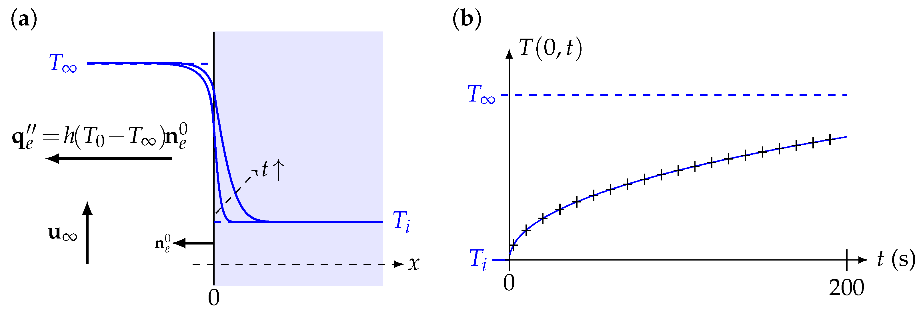
4.1. Heat Point Source

Consider a punctual heat source placed at a point ${\mathrm{M}}^{\prime }$ of Cartesian coordinates $(x^{\prime },y^{\prime },z^{\prime })$, within a stationary, homogeneous, and opaque solid medium (m) of constant physical properties. At each time t, the temperature $T(x,y,z,t)$ of the medium at a point M with coordinates $(x,y,z)$ is written as $T(M,t)=T_0+v(M,t)$, with $v(M,0)=0$ K. Noting $\dot{Q}(M^{\prime },t^{\prime })$ the thermal power emitted by the source point placed at ${\mathrm{M}}^{\prime }$, and the temperature variation $v(M,t)$ is given by the following integral [25]:

$$v(M,t)={\displaystyle \frac{1}{8\rho c{\left(\pi \kappa \right)}^{3/2}}}{\int }_0^t\dot{Q}(M^{\prime },t^{\prime }){\displaystyle \frac{e^{-\frac{r^2}{4\kappa (t-t^{\prime })}}}{{(t-t^{\prime })}^{3/2}}}\mathrm{d}{t}^{\prime },$$

(85)

where $r^2={(x-x^{\prime })}^2+{(y-y^{\prime })}^2+{(z-z^{\prime })}^2$; $\kappa =k/\rho c>0$ is the thermal diffusivity of (m); k, $\rho$, and c are the thermal conductivity, density, and specific heat of (m), respectively. It is also assumed that thermal power is generated by the Joule effect and is written as $\dot{Q}(M^{\prime },t^{\prime })=R(M^{\prime },t^{\prime })i^2\left(t^{\prime }\right)$, where $R(M^{\prime },t^{\prime })$ is the electrical resistance of the source point and $i\left(t\right)$ is the electrical intensity of the heating current. In the present example, the resistance of the source point is assumed to vary linearly with temperature, as is usually the case for examples with metallic materials:

$$R(M^{\prime },t^{\prime })=R_0\left[1+{\alpha }_{T}v(M^{\prime },t^{\prime })\right],$$

(86)

where ${\alpha }_T⩾0$ is the temperature coefficient of the source point. From Equation (85), the temperature $v(M,t)$ is given in this case by the following relation:

$$v(M,t)={\displaystyle \frac{R_0}{8\rho c{\left(\pi \kappa \right)}^{3/2}}}{\int }_0^t{i}^2\left(t^{\prime }\right){\displaystyle \frac{e^{-\frac{r^2}{4\kappa (t-t^{\prime })}}}{{(t-t^{\prime })}^{3/2}}}\mathrm{d}{t}^{\prime }+{\displaystyle \frac{{\alpha }_T{R}_0}{8\rho c{\left(\pi \kappa \right)}^{3/2}}}{\int }_0^t{i}^2\left(t^{\prime }\right)v(M^{\prime },t^{\prime }){\displaystyle \frac{e^{-\frac{r^2}{4\kappa (t-t^{\prime })}}}{{(t-t^{\prime })}^{3/2}}}\mathrm{d}{t}^{\prime }.$$

(87)

Assuming that the point source is spherical, with a radius being a very small compared to the dimensions of the medium (m), located at the origin of the coordinates, the uniform temperature $v\left(t\right)$ of the point source verifies the following integral equation deduced from (87):

$$v\left(t\right)={\displaystyle \frac{R_0}{8\rho c{\left(\pi \kappa \right)}^{3/2}}}{\int }_0^t{i}^2\left(t^{\prime }\right){\displaystyle \frac{e^{-\frac{{\tau }_a}{(t-t^{\prime })}}}{{(t-t^{\prime })}^{3/2}}}\mathrm{d}{t}^{\prime }+{\displaystyle \frac{{\alpha }_T{R}_0}{8\rho c{\left(\pi \kappa \right)}^{3/2}}}{\int }_0^t{i}^2\left(t^{\prime }\right)v\left(t^{\prime }\right){\displaystyle \frac{e^{-\frac{{\tau }_a}{(t-t^{\prime })}}}{{(t-t^{\prime })}^{3/2}}}\mathrm{d}{t}^{\prime },$$

(88)

where ${\tau }_a=a^2/4\kappa$. Assuming that the heating current of the point source is of constant intensity $i\left(t\right)=I_0$, the temperature $v\left(t\right)$ is now given by the following linear Volterra integral equation of the second kind:

$$v\left(t\right)={\displaystyle \frac{R_0{I}_0^2}{8\rho c{\left(\pi \kappa \right)}^{3/2}}}{\int }_0^t{\displaystyle \frac{e^{-\frac{{\tau }_a}{(t-t^{\prime })}}}{{(t-t^{\prime })}^{3/2}}}\mathrm{d}{t}^{\prime }+{\displaystyle \frac{{\alpha }_T{R}_0{I}_0^2}{8\rho c{\left(\pi \kappa \right)}^{3/2}}}{\int }_0^{t}v\left(t^{\prime }\right){\displaystyle \frac{e^{-\frac{{\tau }_a}{(t-t^{\prime })}}}{{(t-t^{\prime })}^{3/2}}}\mathrm{d}{t}^{\prime },$$

(89)

which is of the form (2), with:

$$\lambda ={\displaystyle \frac{{\alpha }_T{R}_0{I}_0^2}{8\rho c{\left(\pi \kappa \right)}^{3/2}}}>0;f\left(t\right)={\displaystyle \frac{\lambda }{{\alpha }_T}}{\int }_0^t{\displaystyle \frac{e^{-\frac{{\tau }_a}{(t-t^{\prime })}}}{{(t-t^{\prime })}^{3/2}}}\mathrm{d}{t}^{\prime };K(t,t^{\prime })={\displaystyle \frac{e^{-\frac{{\tau }_a}{(t-t^{\prime })}}}{{(t-t^{\prime })}^{3/2}}}.$$

(90)

To the best of our knowledge, integral Equation (89) has no analytical solution, so we propose to solve it numerically using the IIRFM, following the various steps shown in Figure 2.

Using the result $\mathcal{L}[e^{-{\tau }_a/t}/t^{3/2}]=\sqrt{\pi /{\tau }_a}{e}^{-2\sqrt{s{\tau }_a}}$, the Laplace transfer function $H_L(s,\lambda )$ of the temperature $v\left(t\right)$ is written as follows, according to (17):

$$H_L(s,\lambda )={\displaystyle \frac{1}{1-\lambda \sqrt{\pi /{\tau }_a}{e}^{-2\sqrt{s{\tau }_a}}}}.$$

(91)

Note that the denominator of the transfer function (91) can have a pole $s_{\lambda }$, given by the following relationship:

$$s_{\lambda }={\displaystyle \frac{ln{\left(\lambda \sqrt{\pi /{\tau }_a}\right)}^2}{4{\tau }_a}}\mathrm{when}{\displaystyle \frac{1}{\lambda }}\sqrt{{\displaystyle \frac{{\tau }_a}{\pi }}}<1.$$

(92)

The transfer function (91) is then decomposed into the form (18), using a Chebyshev rational interpolation. Applying the bilinear transformation finally leads to the result (24), which is written here:

$$v_{\lambda ,f}^{\mathrm{IIR},M}\left(p{T}_e\right)=f\left(p{T}_e\right)+\sum _{i=1}^M{A}_{M,i}\sum _{j=0}^{p-1}{B}_{M,i}^{p-(j+1)}\left[f\left(j{T}_e\right)+f\left((j+1)T_e\right)\right],$$

(93)

with:

$$f\left(j{T}_e\right)={\displaystyle \frac{\lambda }{{\alpha }_T}}{\int }_0^{j{T}_e}{\displaystyle \frac{e^{-\frac{{\tau }_a}{(j{T}_e-t^{\prime })}}}{{(j{T}_e-t^{\prime })}^{3/2}}}\mathrm{d}{t}^{\prime }={\displaystyle \frac{R_0{I}_0^2}{4\pi ka}}\mathrm{erfc}\left(\sqrt{{\displaystyle \frac{{\tau }_a}{j{T}_e}}}\right),$$

(94)

where the coefficients $A_{M,i}$ and $B_{M,i}$ have the usual expressions introduced in the previous paragraphs. Note that in the limit where ${\alpha }_T\to 0$ (case of constant electrical resistance), the temperature $v\left(t\right)$ is then identified with the function $f\left(t\right)$.

Figure 14 shows the time variations in temperature $v\left(t\right)$ of a heat point source with radius $a=0.5$ mm, immersed in ethylene glycol at rest, at room temperature ($\rho =1113.5\mathrm{kg}/{\mathrm{m}}^3,$$k=0.254\mathrm{W}/\mathrm{m}/\mathrm{K}$, $c=2380\mathrm{J}/\mathrm{K}/\mathrm{kg}$). The electrical heating current considered had a constant intensity $I_0=250\mathrm{mA}$ and the temperature coefficient of the point source was ${\alpha }_T=0.0039{\mathrm{K}}^{-1}$, for an electrical resistance $R_0=1\Omega$. The Chebyshev interpolation $H_{\mathrm{L}}^M(s,\lambda )$ was calculated with $M=4$, over the interpolation interval $I_s=[0,5]{\mathrm{Hz}}^{-1}$. The maximal relative error ${\epsilon }_r^{\max }$ committed on the approximation of $H_{\mathrm{L}}(s,\lambda )$ was in this case ${\epsilon }_r^{\max }=0.058\%$ for $s\in [{10}^{-2},{10}^2]{\mathrm{Hz}}^{-1}$. The sampling period was $T_e=0.01$ s.

Figure 14. Time changes in the temperature $v\left(t\right)$ of a Joule-heated source point at constant intensity, calculated using the IIRFM (relations (93) and (94)).

From the results shown in Figure 14, it can be seen that the temperature coefficient ${\alpha }_T$ has a non-negligible influence on the time evolution of the source point temperature. When the influence of ${\alpha }_T$ is taken into account, the self-heating of the source point leads to an increase in its electrical resistance (because ${\alpha }_T$ is positive), and so at constant heating intensity, this leads to an increase in the Joule heating power and consequently in its temperature $v\left(t\right)$, compared to the situation where ${\alpha }_T=0$. These observations could be applied to various methods of the thermal characterization of materials.

4.2. Surface Temperature of Semi-Infinite Solids

The IIRFM is now applied to the solution of the linear integral equation verified by the interface temperature of a semi-infinite isotropic solid (defined by $x>0$), of uniform initial temperature $T_i$, subjected to mixed (or Robin, see Figure 15a) boundary conditions at $x=0$.

Figure 15. Temperature of a semi-infinite solid ($x>0$) with constant Robin boundary conditions at $x=0$, due to a fluid flowing at constant velocity ${\mathbf{u}}_{\infty }$ and temperature $T_{\infty }$ far from the solid, with constant Newton coefficient h. (a) Temperature profiles at different times, for $T_{\infty }>T_i$. (b) Time evolution of the $T(0,t)$ surface temperature when $T_{\infty }=\mathrm{cste}$. The symbols correspond to the analytical solution (100) and the solid line to the numerical solution (102) obtained by the IIRFM method.

The temperature field $\theta (x,t)=T(x,t)-T_i$ in this case satisfies the usual heat equation without a source term, as follows:

$${\displaystyle \frac{\partial \theta }{\partial t}}=\kappa {\displaystyle \frac{{\partial }^2\theta }{\partial x^2}}\mathrm{with}\theta (x,0)=0\mathrm{and}\theta (+\infty ,t)<\infty ,$$

(95)

where $\kappa =k/\rho c>0$ is the thermal diffusivity of the solid, assumed constant. Applying the Laplace transformation to Equation (95) leads to the ordinary differential equation ${\mathrm{d}}_{x^2}\overline{\theta }(x,s)-{\displaystyle \frac{s}{\kappa }}\overline{\theta }(x,s)=0$, of which the solution is written in the general form $\overline{\theta }(x,s)=A{e}^{-\sqrt{s/\kappa }x}+B{e}^{\sqrt{s/\kappa }x}$, with $\overline{\theta }(x,s)=\mathcal{L}\left[\theta (x,t)\right]$. The finite boundary condition $\theta (+\infty ,t)<\infty$ implies $B=0$ here.

Let us note ${\mathbf{q}}_e^{\prime \prime }(0,t)=q_e^{\prime \prime }\left(t\right){\mathbf{n}}_e^0$, the heat flux exchanged by the solid with the external fluid at $x=0$. The continuity of heat fluxes at the interface $x=0$ is written as ${\mathbf{q}}_e^{\prime \prime }(0,t)=-k{\partial }_{n_e^0}T{\mathbf{n}}_e^0=-k{\partial }_{n_e^0}\theta {\mathbf{n}}_e^0$. Applying the Laplace transformation to the continuity relation leads to the following expression for $\overline{\theta }(x,s)$:

$$\overline{\theta }(x,s)=-{\displaystyle \frac{\sqrt{\kappa }}{k}}{\overline{q}}_e^{\prime \prime }\left(s\right){\displaystyle \frac{e^{-\sqrt{s/\kappa }x}}{\sqrt{s}}},$$

(96)

where ${\overline{q}}_e^{\prime \prime }\left(s\right)=\mathcal{L}\left[q_e^{\prime \prime }\left(t\right)\right]$. By recalling that ${\mathcal{L}}^{-1}\left[e^{-\beta \sqrt{s}}/\sqrt{s}\right]=e^{-{\beta }^2/4t}/\sqrt{\pi t}$ and applying the convolution theorem, it is possible to invert $\overline{\theta }(x,s)$ and write $\theta (x,t)$ in the form of the following convolution integral:

$$\theta (x,t)=-{\displaystyle \frac{1}{k}}\sqrt{{\displaystyle \frac{\kappa }{\pi }}}{\int }_0^t{\displaystyle \frac{q_e^{\prime \prime }\left(\tau \right)}{{(t-\tau )}^{1/2}}}{e}^{-{\displaystyle \frac{x^2}{4\kappa (t-\tau )}}}\mathrm{d}\tau .$$

(97)

Finally, using Newton’s law ${\mathbf{q}}_e^{\prime \prime }(0,t)=h\left[\theta \left(0,t\right)-{\theta }_{\infty }\left(t\right)\right]{\mathbf{n}}_e^0$ leads to the following expression of $\theta (x,t)$:

$$\theta (x,t)={\displaystyle \frac{h}{k}}\sqrt{{\displaystyle \frac{\kappa }{\pi }}}{\int }_0^t{\displaystyle \frac{{\theta }_{\infty }\left(\tau \right)-\theta (0,\tau )}{{(t-\tau )}^{1/2}}}{e}^{-{\displaystyle \frac{x^2}{4\kappa (t-\tau )}}}\mathrm{d}\tau ,$$

(98)

where the Newton coefficient h is assumed to be constant. According to result (98), the surface temperature $\theta (0,t)$ finally verifies the following Abel integral equation of the second kind:

$$\theta (0,t)=f\left(t\right)+\lambda {\int }_0^t{\displaystyle \frac{\theta (0,\tau )}{{(t-\tau )}^{1/2}}}\mathrm{d}\tau ,$$

(99)

with $\lambda =-{\displaystyle \frac{h}{k}}\sqrt{{\displaystyle \frac{\kappa }{\pi }}}<0$ and $f\left(t\right)={\displaystyle \frac{h}{k}}\sqrt{{\displaystyle \frac{\kappa }{\pi }}}{\int }_0^t{\displaystyle \frac{{\theta }_{\infty }\left(\tau \right)}{{(t-\tau )}^{1/2}}}\mathrm{d}\tau$.

In the following paragraphs, Equation (99) is solved by the IIRFM for two different expressions of the temperature $T_{\infty }\left(t\right)$ of the fluid far from the solid wall.

4.2.1. First Application: $T_{\infty }\left(t\right)=\mathrm{cste}$

First, consider the usual case where the temperature $T_{\infty }$ of the fluid far from the solid wall $x=0$ is constant. In this case, it is found that $f\left(t\right)={\displaystyle \frac{2h}{k}}{\theta }_{\infty }\sqrt{\kappa /\pi }\sqrt{t}=f_{\infty }{t}^n$ with $n=1/2$ and ${\theta }_{\infty }=T_{\infty }-T_i$. Equation (99) then admits an analytical solution ${\theta }_a\left(t\right)=T(0,t)-T_i$ involving the complementary error function:

$${\displaystyle \frac{{\theta }_a\left(t\right)}{{\theta }_{\infty }}}=1-exp\left({\displaystyle \frac{h^2\kappa t}{k^2}}\right)\mathrm{erfc}\left({\displaystyle \frac{h\sqrt{\kappa t}}{k}}\right).$$

(100)

Equation (99) is solved in the following by the IIRFM, using the general result (24). First of all, it is possible here to determine an explicit expression ${\Xi }_{N,i}$ for the sum ${\sum }_{j=0}^{k-1}{B}_{N,i}^{k-(j+1)}\left[f\left(j{T}_e\right)+f\left((j+1)T_e\right)\right]$, in the general case where $f\left(t\right)=f_{\infty }{t}^n$:

$${\Xi }_{N,i}\left(k,T_e,B_{N,i},f\right)=f_{\infty }{T}_e^n\left\{B_{N,i}^{k-1}\left(1+B_{N,i}\right){\mathrm{Li}}_{-n}\left(B_{N,i}^{-1}\right)+k^n-(1+B_{N,i}^{-1})\Phi \left(B_{N,i}^{-1},-n,k\right)\right\},$$

(101)

where the polylogarithm Li and transcendent Lerch $\Phi$ functions were defined in Section 3.1.1. Using result (101) with $n=1/2$, the following explicit expression is obtained for the IIRFM solution to the problem (99), at time $t_k=k{T}_e$ (with $k⩾1$):

$$\begin{array}{cc}\hfill {\displaystyle \frac{{\theta }_{\sqrt{t}{f}_{\infty }}^{\mathrm{IIR},N}\left(t_k\right)}{f_{\infty }\sqrt{T_e}}}& =\sqrt{k}+\hfill \\ \hfill & \sum _{i=1}^N{A}_{N,i}\left[B_{N,i}^{k-1}\left(1+B_{N,i}\right){\mathrm{Li}}_{-{\displaystyle \frac{1}{2}}}\left(B_{N,i}^{-1}\right)+\sqrt{k}-(1+B_{N,i}^{-1})\Phi \left(B_{N,i}^{-1},-{\displaystyle \frac{1}{2}},k\right)\right].\hfill \end{array}$$

(102)

The thermal problem (99), of calculating the surface temperature of a semi-infinite solid surrounded by a fluid, is solved using result (102) for the following physical properties: $k=40\mathrm{W}·{\mathrm{K}}^{-1}·{\mathrm{m}}^{-1}$; $\rho =7850\mathrm{kg}·{\mathrm{m}}^{-3}$; $c=490\mathrm{J}·{\mathrm{K}}^{-1}·{\mathrm{kg}}^{-1}$; $\kappa =1.04·{10}^{-5}{\mathrm{m}}^2·{\mathrm{s}}^{-1}$; for Newton coefficient $h=100\mathrm{W}·{\mathrm{K}}^{-1}·{\mathrm{m}}^{-2}$; $t\in [0,200]\mathrm{s}$; and $T_e=1$ s. Numerical (continuous line) and analytical results ( + symbols) are shown in Figure 15b. From this figure it can be seen that there is a good correspondence between the IIRFM numerical solution and the analytical solution. This good agreement is confirmed by the low values of the maximal error ${\epsilon }_{\infty ,N_t}^{\mathrm{IIR}}=1.41·{10}^{-4}$ K and root mean square error ${\epsilon }_{2,N_t}^{\mathrm{IIR}}=1.58·{10}^{-5}$ K, with

$${\epsilon }_{2,N_t}^{\mathrm{IIR}}=\sqrt{{\displaystyle \frac{1}{N_t+1}}{\sum }_{k=0}^{N_t}{\left({\theta }_a\left(t_k\right)-{\theta }_{\sqrt{t}{f}_{\infty }}^{\mathrm{IIR},N}\left(t_k\right)\right)}^2}\mathrm{and}{\epsilon }_{\infty ,N_t}^{\mathrm{IIR}}=\underset{\mathcal{S}}{max}\left|{\theta }_a-{\theta }_{\sqrt{t}{f}_{\infty }}^{\mathrm{IIR},N}\right|,$$

(103)

where $\mathcal{S}$ is the set of points $\left\{{\left(t_k,{\theta }_{\sqrt{t}{f}_{\infty }}^{\mathrm{IIR},N}\left(t_k\right)\right)}_{n=0}^{N_t}\right\}$ obtained using the IIRFM method.

4.2.2. Second Application: $T_{\infty }\left(t\right)={\widehat{T}}_{\infty }sin\left(\omega t\right)$

Thermal problem (99) is still considered, but now for a sinusoidal temperature $T_{\infty }\left(t\right)$ with pulsation $\omega$: $T_{\infty }\left(t\right)={\widehat{T}}_{\infty }sin\left(\omega t\right)$, all other things being equal to what was considered in the previous example. The $f\left(t\right)$ function in Equation (99) becomes here

$$\begin{array}{cc}\hfill f\left(t\right)& =-\lambda {\widehat{\theta }}_{\infty }{\int }_0^t{\displaystyle \frac{sin\left(\omega \tau \right)}{{(t-\tau )}^{1/2}}}\mathrm{d}\tau ,\hfill \\ \hfill & =-\lambda {\widehat{\theta }}_{\infty }\sqrt{{\displaystyle \frac{\pi }{\omega }}}\left[\mathrm{FC}\left(\sqrt{{\displaystyle \frac{2\omega t}{\pi }}}\right)sin\left(\omega t\right)-\mathrm{FS}\left(\sqrt{{\displaystyle \frac{2\omega t}{\pi }}}\right)cos\left(\omega t\right)\right],\hfill \end{array}$$

(104)

where $\lambda =-{\displaystyle \frac{h}{k}}\sqrt{\kappa /\pi }$; ${\widehat{\theta }}_{\infty }={\widehat{T}}_{\infty }-T_i$; $\mathrm{FC}$ and $\mathrm{FS}$ are the Fresnel integrals. An analytical solution ${\theta }_a\left(t\right)$ also exists here, and can be obtained by inverting the Laplace transform $\overline{\theta }(0,s)={\displaystyle \frac{{\widehat{\theta }}_{\infty }\omega }{s^2+{\omega }^2}}/\left(1+{\displaystyle \frac{k\sqrt{s}}{h\sqrt{\kappa }}}\right)$:

$$\begin{array}{cc}\hfill {\displaystyle \frac{{\theta }_a\left(t\right)}{{\widehat{\theta }}_{\infty }}}& ={\displaystyle \frac{h^4{\kappa }^{2}sin\left(\omega t\right)+h^2{k}^2\kappa \omega \left[cos\left(\omega t\right)-e^{\frac{h^2\kappa t}{k^2}}\mathrm{erfc}\left(\frac{h\sqrt{\kappa t}}{k}\right)\right]}{h^4{\kappa }^2+k^4{\omega }^2}}\hfill \\ \hfill & +{\displaystyle \frac{hk\sqrt{2\kappa \omega }}{h^4{\kappa }^2+k^4{\omega }^2}}\mathrm{FC}\left(\sqrt{{\displaystyle \frac{2\omega t}{\pi }}}\right)\left[k^2\omega sin\left(\omega t\right)-h^2\kappa cos\left(\omega t\right)\right]\hfill \\ \hfill & -{\displaystyle \frac{hk\sqrt{2\kappa \omega }}{h^4{\kappa }^2+k^4{\omega }^2}}\mathrm{FS}\left(\sqrt{{\displaystyle \frac{2\omega t}{\pi }}}\right)\left[h^2\kappa sin\left(\omega t\right)+k^2\omega cos\left(\omega t\right)\right].\hfill \end{array}$$

(105)

Figure 16 compares the numerical results (solid line) obtained by the IIRFM to the results provided (black dashes) by the analytical expression (105), when $\omega =2\pi /T_h$ with $T_h=12\mathrm{h}$ and $t\in [0,t_f=6T_h]$. The correspondence between the results provided by the IIRFM and the analytical solution is again very good, with maximum error ${\epsilon }_{\infty ,N_t}^{\mathrm{IIR}}=3.72·{10}^{-3}$ K and root mean square error ${\epsilon }_{2,N_t}^{\mathrm{IIR}}=1.25·{10}^{-3}$ K, calculated for a sampling period $T_e=216\mathrm{s}$.

Figure 16. Time changes in the surface temperature $\theta (0,t)$ of a semi-infinite solid, for sinusoidal variations ${\theta }_{\infty }\left(t\right)={\widehat{\theta }}_{\infty }sin\left(\omega t\right)$ of the fluid temperature far from the solid and for a constant flow velocity ${\mathbf{u}}_{\infty }$.

5. Conclusions

In this work, the first-order infinite impulse response filters method (IIRFM), usually reserved for the study of linear ordinary differential equations with constant coefficients, has been extended to the numerical solution of various linear Volterra convolution integral equations (VCIE) of the second kind. A wide variety of examples have been studied, illustrating the great flexibility of the IIRFM. Three types of convolutive kernels were discussed in detail in this work: unit, Abel, and logarithmic kernels.

In the case of the unit kernel, the IIRFM was compared to the homotopic perturbation method with Laplace transform (HPM-L). The HPM-L method has the great advantage of leading, for certain special cases, to an analytic solution of the linear convolutive Volterra integral equation of the second kind. However, due to its iterative nature, the numerical version of the HPM-L method may exhibit convergence speeds that are far too low to allow, in the absence of an analytical solution, an efficient numerical resolution of certain VCIEs. In contrast, we have observed that the IIRFM leads, in the case of the unit kernel, to numerical solutions that do not exhibit convergence problems. In many cases, it has also been possible to provide a simple, highly efficient analytical expression for the IIRFM numerical solution.

In the case of the Abel kernel, the numerical results provided by the IIRFM approach have been compared with the results provided by various recent numerical methods (Daubechies wavelets and approximations based on Laguerre polynomials). For most of the comparisons examined, the IIRFM proved to be the best-performing and most consistent overall.

Finally, the IIRFM has been applied to the numerical solution of Volterra integral equations of the second kind encountered in two linear thermal problems. In addition, a new approximate expression for the pathological function $g_{\lambda }\left(t\right)=1+\mathrm{erf}\left(\lambda \sqrt{\pi t}\right)$ has been proposed, giving accurate results for $\lambda <0$, even using single-precision floating-point numbers.

In a forthcoming paper, the IIRFM will be extended to the numerical solution of the non-linear Volterra convolution integral equations of the second kind. It will also be very interesting to consider the application of the IIRFM to fractional differential or integral equations [26].

References

- De, S.; Mandal, B.; Chakrabarti, A. Use of Abel integral equations in water wave scattering by two surface-piercing barriers. Wave Motion 2010, 47, 279–288. [Google Scholar] [CrossRef]
- Mirceski, V.; Tomovski, Z. Analytical solutions of integral equations for modelling of reversible electrode processes under voltammetric conditions. J. Electroanal. Chem. 2008, 619–620, 164–168. [Google Scholar] [CrossRef]
- Wazwaz, A.M. Linear and Nonlinear Integral Equations—Methods and Applications; Springer: Berlin/Heidelberg, Germany, 2011. [Google Scholar]
- Polyanin, A.D.; Manzhirov, A.V. Handbook of Integral Equations, 2nd ed.; Chapman and Hall/CRC: Boca Raton, FL, USA, 2008. [Google Scholar]
- Kumar, S.; Kumar, A.; Kumar, D.; Singh, J.; Singh, A. Analytical solution of Abel integral equation arising in astrophysics via Laplace transform. J. Egypt. Math. Soc. 2015, 23, 102–107. [Google Scholar] [CrossRef]
- Thota, S. Solution of Generalized Abel’s Integral Equations by Homotopy Perturbation Method with Adaptation in Laplace Transformation. Sohag J. Math. 2022, 9, 29–35. [Google Scholar]
- Chowdhury, M.S.H.; Mohamed, M.S.; Gepreel, K.A.; Al-Malki, F.A.; Al-Humyani, M. Approximate Solutions of the Generalized Abel’s Integral Equations Using the Extension Khan’s Homotopy Analysis Transformation Method. J. Appl. Math. 2015, 2015, 357861. [Google Scholar]
- Liao, S. On the homotopy analysis method for nonlinear problems. Appl. Math. Comput. 2004, 147, 499–513. [Google Scholar] [CrossRef]
- Liao, S. Comparison between the homotopy analysis method and homotopy perturbation method. Appl. Math. Comput. 2005, 169, 1186–1194. [Google Scholar] [CrossRef]
- Bairwa, R.K.; Kumar, A.; Kumar, D. An Efficient Computation Approach for Abel’s Integral Equations of the Second Kind. Sci. Technol. Asia 2020, 25, 85–94. [Google Scholar]
- Heyd, R. Real-time heat conduction in a self-heated composite slab by Padé filters. Int. J. Heat Mass Transf. 2014, 71, 606–614. [Google Scholar] [CrossRef]
- Lahboub, D.; Heyd, R.; Bakak, A.; Lotfi, M.; Koumina, A. Solution of Basset integro-differential equations by IIR digital filters. Alex. Eng. J. 2022, 61, 11899–11911. [Google Scholar] [CrossRef]
- Mouley, J.; Panja, M.M.; Mandal, B.N. Approximate solution of Abel integral equation in Daubechies wavelet basis. CUBO A Math. J. 2021, 23, 245–264. [Google Scholar] [CrossRef]
- Singha, N.; Nahak, C. Solutions of the Generalized Abel’s Integral Equation using Laguerre Orthogonal Approximation. Appl. Appl. Math. Int. J. (AAM) 2019, 14, 1051–1066. [Google Scholar]
- Adomian, G.; Rach, R. Noise terms in decomposition series solution. Comput. Math. Appl. 1992, 24, 61–64. [Google Scholar] [CrossRef]
- Adomian, G. Solving Frontier Problems of Physics: The Decomposition Method; Kluwer: Alphen aan den Rijn, The Netherlands, 1994. [Google Scholar]
- He, J.H. Homotopy perturbation technique. Comput. Methods Appl. Mech. Eng. 1999, 178, 257–262. [Google Scholar] [CrossRef]
- He, J.H. A coupling method of a homotopy technique and a perturbation technique for non-linear problems. Int. J. Non-Linear Mech. 2000, 35, 37–43. [Google Scholar] [CrossRef]
- He, J.H. Homotopy perturbation method: A new nonlinear analytical technique. Appl. Math. Comput. 2003, 135, 73–79. [Google Scholar] [CrossRef]
- Madani, M.; Fathizadeh, M. Homotopy Perturbation Algorithm using Laplace Transformation. Nonlinear Sci. Lett. A 2010, 1, 263–267. [Google Scholar]
- Khan, Y.; Wu, Q. Homotopy perturbation transform method for nonlinear equations using He’s polynomials. Comput. Math. Appl. 2011, 61, 1963–1967. [Google Scholar] [CrossRef]
- Singh, J.; Kumar, D.; Rathore, S. Application of Homotopy Perturbation Transform Method for Solving Linear and Nonlinear Klein-Gordon Equations. J. Inf. Comput. Sci. 2012, 7, 131–139. [Google Scholar]
- Heyd, R.; Hadaoui, A.; Saboungi, M. 1D analog behavioral SPICE model for hot wire sensors in the continuum regime. Sens. Actuators A Phys. 2012, 174, 9–15. [Google Scholar] [CrossRef]
- Lotfi, M.; Mezrigui, L.; Heyd, R. Study of heat conduction through a self-heated composite cylinder by Laplace transfer functions. Appl. Math. Model. 2016, 40, 10360–10376. [Google Scholar] [CrossRef]
- Carslaw, H.; Jaeger, J.C. Conduction of Heat in Solids; Oxford University Press: Oxford, UK, 1959. [Google Scholar]
- Zhao, K.; Liu, J.; Lv, X. A Unified Approach to Solvability and Stability of Multipoint BVPs for Langevin and Sturm–Liouville Equations with CH-Fractional Derivatives and Impulses via Coincidence Theory. Fractal Fract. 2024, 8, 111. [Google Scholar] [CrossRef]
Disclaimer/Publisher’s Note: The statements, opinions and data contained in all publications are solely those of the individual author(s) and contributor(s) and not of MDPI and/or the editor(s). MDPI and/or the editor(s) disclaim responsibility for any injury to people or property resulting from any ideas, methods, instructions or products referred to in the content. |
© 2024 by the author. Licensee MDPI, Basel, Switzerland. This article is an open access article distributed under the terms and conditions of the Creative Commons Attribution (CC BY) license (https://creativecommons.org/licenses/by/4.0/).