Article

Customized Bus Stop Location Model Based on Dual Population Adaptive Immune Algorithm

1
SILC Business School, Shanghai University, No.20 Chengzhong Road, Shanghai 201800, China
2
School of Computer Science and Technology, Xi’an Jiaotong University, No.28 Xianning West Road, Xi’an 710049, China
3
School Administrative Office, Northwestern Polytechnical University, Xi’an 710127, China
4
School of Naval Architecture, Ocean & Civil Engineering, Shanghai Jiaotong University, No.800 Dongchuan Road, Shanghai 200240, China
*
Authors to whom correspondence should be addressed.
Mathematics 2024, 12(15), 2382; https://doi.org/10.3390/math12152382
Submission received: 5 June 2024 / Revised: 12 July 2024 / Accepted: 29 July 2024 / Published: 31 July 2024

Abstract

:
Selecting optimal locations for customized bus stops is crucial for enhancing the adoption rate of customized bus services, reducing operational costs, and, consequently, mitigating traffic congestion. This study leverages ride-hailing data to analyze the distance between passengers and bus stops, as well as the operational costs associated with establishing these stops, to construct a customized bus stop location model. To address the limited local search capability of conventional immune algorithms, we propose a Dual Population Adaptive Immunity Algorithm (DPAIA) to solve the bus stop location problem. Finally, we conduct simulation experiments using passenger travel data from a ride-hailing company in Chengdu to evaluate the proposed customized bus stop location model. Through simulations with Chengdu ride-hailing data, the DPAIA algorithm minimized the weighted cost to CNY 28.95 ten thousand, outperforming all counterparts. Although proposing 9–11 more stops than competitors, this increase slightly impacts costs while markedly reducing passenger walking distances. Optimizing station placement to meet demand and road networks, our model endorses 50 strategic bus stops, enhancing service accessibility and potentially easing urban congestion while boosting operator profits.

1. Introduction

Customized bus services, derived from the concept of shared mobility abroad, have emerged as a novel tool for passenger transportation. Their primary function lies in providing convenient and comfortable travel options for passengers with similar starting points and travel times. The emergence of customized bus services not only offers passengers fast, flexible, and high-quality transportation but also holds significant importance in alleviating urban traffic pressure. To fully leverage the service advantages of customized bus services, it is imperative to conduct rational planning for their stop locations.
From existing research, L. Xu et al. [1] proposed a real-time search algorithm for studying real-time optimization problems of customized bus stations to maximize customer service rate and operator profit. Chen et al. [2] developed a dynamic programming model based on nonlinear integer programming to study boarding and docking scheduling problems at different library stations. Huo et al. [3] conducted positioning research on customized bus services in Beijing using Didi data, involving the identification of peak travel periods, screening spatial outliers, partitioning traffic zones, identifying OD characteristics, and selecting customized bus stop locations. Xue et al. [4] proposed a two-step optimization scheme for bus stop locations, analyzing user walking and waiting cycles to determine alternative areas for transfer and ridesharing stations. Wang et al. [5] presented a method for stop location selection considering the complexity of service areas and the uncertainty of routes in customized bus services. Liu et al. [6] introduced a block clustering algorithm based on passenger distribution and route direction, incorporating weighted hierarchical clustering into their algorithm. Density-Based Spatial Clustering of Applications with Noise (DBSCAN) is a prominent data clustering algorithm that stands out for its ability to discover clusters of arbitrary shapes in spatial databases [7]. Unlike traditional clustering methods such as k-means, which require the number of clusters to be predefined, DBSCAN identifies clusters based on density, automatically determining the number of clusters based on the data’s inherent structure. Liu et al. [8] improved the DBSCAN algorithm for customized bus stop location selection by enhancing the calculation of demand point distances, selecting clustering parameters, and choosing cluster centers. Zhang et al. [9] utilized an improved AP clustering method, introducing an adjustment factor to solve the clustering center based on the frequency of customized bus stop applications. Sun et al. [10] employed an improved DBSCAN clustering method to finely divide densely populated areas serviced by customized buses, further analyzing intra-cluster dispersion and inter-cluster significance.
In summary, most scholars have tackled the problem of customized bus stop location selection using clustering methods. However, clustering methods typically focus solely on spatial factors in solving this problem, overlooking the variability in distances between passengers and bus stops or assuming fixed values, which does not adequately reflect real-world conditions. Moreover, although many models employ population-based intelligent optimization algorithms, which offer robust global search capabilities and high computational efficiency, they often exhibit limited local search mechanisms and may struggle with local optima. Therefore, this paper addresses the modeling of customized bus stop location selection, constructs a multi-objective optimization function, and then improves immune algorithms for solving stop location models. Finally, the rationality of the proposed stop location model and solution algorithm is validated through simulation experiments.

2. Problem Description

2.1. Description of Customized Bus Stop Location Problem

In the problem of determining customized bus stop locations, spatial factors are generally the predominant focus, resulting in the problem being treated as a single-objective optimization issue. Furthermore, the distance between passengers and bus stops is frequently disregarded or set as a constant, which is inconsistent with real-world conditions. This paper addresses the dual objective of balancing passenger travel demands and operator economic interests in the selection of customized bus stop locations. The primary aim is to reduce both the walking costs for passengers and the costs associated with constructing customized bus stations.
The proposed solution is to minimize the weighted sum of operator costs and passenger travel costs by carefully selecting customized bus stop locations. The model assumes that each travel point in the ride-hailing data represents a demand, and passengers with ride demands within a certain geographical area and time frame are grouped to board customized buses at the same stop. The objective is to ensure that the location of these stops is optimal and practical for both passengers and operators.

2.2. Assumptions of the Customized Bus Stop Location Model

For operators, considering the varying costs associated with establishing stops in different areas and residential environments, it is essential to minimize the number of stops to reduce operator costs. For passengers, when they need to take a customized bus, they must walk to the nearest bus stop. The walking distance should not be too far, and when there are multiple stops within walking distance, passengers must choose one stop. Once they choose a stop, they cannot select another. To facilitate calculations, the model makes the following reasonable assumptions based on engineering practicality:
(1)
Each passenger can only go to one customized bus stop.
(2)
After choosing a bus stop, passengers will not select another customized bus stop.
(3)
The number of passengers accommodated at a customized bus stop cannot exceed its capacity.
(4)
The cost of establishing a customized bus stop cannot exceed the maximum budget.
(5)
The walking distance from passengers to the bus stop cannot exceed the maximum distance covered by the stop.

2.3. Processing of Customized Bus Passenger Travel Data

Currently, the process of selecting customized bus stop locations often resembles the approach used for regular bus stops, which is primarily based on traffic zone partitioning. This method, which considers commercial and residential areas as potential passenger travel points, does not adequately reflect real-world dynamics. To address this gap, our study proposes converting ride-hailing data into customized bus travel demand data to better align with actual travel patterns and potentially reduce traffic congestion. This approach is grounded in the understanding that ride-hailing data can accurately capture passenger demand characteristics. Thus, this paper utilizes ride-hailing data to inform the selection of customized bus stop locations.

2.3.1. Acquisition of Customized Bus Passenger Travel Data

Customized bus passenger travel demands are analyzed through the analysis of ride-hailing data. The acquisition of ride-hailing data in the region primarily includes basic information, such as terminal numbers and terminal phone numbers of passengers and drivers; ride-hailing vehicle status, including whether the vehicle is in motion and its speed; and ride-hailing vehicle geographical location, which includes longitude and latitude at the current positioning time. The geographical location of ride-hailing vehicles is updated every 30 s when the ACC status is on, and every 5 min otherwise.

2.3.2. Processing of Customized Bus Passenger Travel Data

Abnormal data within the obtained ride-hailing data in the region are processed. For instance, data anomalies may include missing ride-hailing vehicle locations, abnormal ride-hailing vehicle locations, missing ride-hailing vehicle times, and other data anomalies. Additionally, similar duplicate roads may exist. Data correction methods are employed to address these issues, with primary processing measures outlined in Table 1.
For the data corrected using the data correction method, the corresponding geographical locations such as longitude and latitude are searched, and they are transformed into mathematical definitions according to Equation (1).
V m = { A x m j z , O x m j z , A m j z , O m j z , t m e o , t m a o }
In the equation, m represents the travel demand index; A x m j z denotes the longitude coordinate of the passenger’s starting point; O x m j z represents the latitude coordinate of the passenger’s starting point; A m j z denotes the longitude coordinate of the passenger’s destination; O m j z represents the latitude coordinate of the passenger’s destination; t m e o denotes the departure time of the passenger; t m a o represents the arrival time of the passenger.

3. Model Construction

A strategic selection of customized bus stop locations can significantly improve passenger convenience while maximizing operator cost-efficiency, leading to increased adoption of customized bus services. As more passengers opt for these services, the approach contributes to reducing urban traffic congestion. Consequently, when determining the optimal bus stop locations, it is essential to balance the walking distance for passengers with the construction costs for operators. Based on these considerations, the objective function and constraints for the selection model of customized bus stop locations and route planning are proposed.

3.1. Objective Function of the Customized Bus Stop Location Model

In the customized bus stop location problem, for passengers, the objective is to minimize walking distance as much as possible, while for operators, the aim is to plan the number of stops reasonably and control the economic costs of building stops. The objective function of the customized bus stop location model is represented by Equations (2) and (3):
min D = i N j G i g i h i j X i j + j G j l j v j
x i j = { 1 ,   p a s s e n g e r   i   i s   a s s o c i a t e d   w i t h   s t a t i o n   j 0 ,   p a s s e n g e r   i   i s   n o t   a s s o c i a t e d   w i t h   s t a t i o n   j
In the equations, N represents the set of passenger demand sequences, G i represents the set of candidate stations meeting the distance condition between passengers and stations, g i represents the walking distance cost for passengers, h i j represents the distance between passengers and stations, x i j represents the matching relationship between passengers and stations, l j represents the cost of establishing station j , v j represents whether a station j is selected as a candidate stop for customized buses, passenger i is not associated with station j.

3.2. Constraints of the Customized Bus Stop Location Model

After selecting appropriate objective functions, constraints on the number of stations and the distance between passengers and stations are necessary to enhance attractiveness to passengers. The constraints of the customized bus stop location model established in this paper are as follows:
Constraint 1. A passenger cannot simultaneously go to multiple bus stops. Therefore, each passenger can only go to one customized bus stop, defined as follows in Equation (4):
j G I X i j = 1 , i N
Constraint 2. For passengers, once they select a bus stop and travel to it, they wait for the arrival of the customized bus and do not choose to go to other stops on the same route to wait for the bus. This is defined as shown in Equations (5) and (6):
X i j v j , i N ; j G
v j = { 1 ,   s e l e c t i n g   s t a t i o n   j   a s   a   c a n d i d a t e   s t a t i o n 0 ,   n o t   s e l e c t i n g   s t a t i o n   j   a s   a   c a n d i d a t e   s t a t i o n
In the equation, v j is a Boolean variable that indicates whether the point j is selected as a candidate location for a bus stop.
Constraint 3. The cost of establishing customized bus stops must not exceed the maximum budget. A reasonable maximum cost is set, defined as shown in Equation (7):
j G j l j v j M
In the equation, M represents the maximum cost that can be spent on establishing customized bus stops.
Constraint 4. The walking distance from passengers to the bus stop must not exceed the maximum distance covered by the stop. A reasonable maximum walking distance is set, defined as shown in Equation (8):
h i j R
In the equation, R represents the maximum distance that passengers can walk to the bus stop, which is the coverage radius of the stop.

4. Algorithm Design

4.1. Principle of Dual Population Adaptive Immunity Algorithm (DPAIA)

The Immune Algorithm (IA) is an intelligent optimization algorithm inspired by the biological immune system and incorporates the evolutionary mechanisms of genes. IA iterates multiple times through processes such as initializing populations, calculating fitness, immune operations, and generating new populations, employing a population search strategy. Eventually, it tends to find the optimal solution to the problem with a high probability. This algorithm possesses advantages such as global convergence, parallelism, and adaptability. IA has strong global search capabilities, robustness, and a parallel distributed search mechanism [11], making it suitable for solving the stop model.
However, IA lacks an effective local search mechanism, and it is challenging to determine suitable values for the crossover rate and mutation rate in immune operations. To address these shortcomings, this paper proposes an improvement to the IA, introducing the Dual Population Adaptive Immunity Algorithm (DPAIA). This algorithm aims to enhance the local search capability and convergence speed by incorporating two populations and adaptive mechanisms. The DPAIA algorithm is utilized to solve the model, thereby identifying reasonable candidate locations for customized bus stops.
Specific Improvement Points are as follows.

4.1.1. Setting Adaptive Crossover Rate and Mutation Rate

In immune operations, the convergence of the immune algorithm is influenced by both the crossover rate and the mutation rate. The crossover rate is positively correlated with the antibody generation rate. A higher crossover rate leads to a faster antibody generation rate, while a lower crossover rate slows down the algorithm’s search speed, affecting computational time. If the mutation rate is too small, it is difficult to generate new individuals, whereas if it is too large, the algorithm may become a completely random search algorithm. The values of the crossover rate and mutation rate often need to be validated through numerous experiments for different problems. It is challenging to obtain reasonable values in a short period. Therefore, this paper proposes adaptive crossover rates and mutation rates to reduce the computational cost of the model and improve its efficiency.
There are three forms of immune operations: selection, crossover, and mutation. For selection operations, this paper adopts the roulette wheel selection method, where the probability of individual selection is consistent with the expected reproduction rate. The expected reproduction rate is calculated as follows:
p v , w = γ C v , w C v , w + ( 1 γ ) C v , w C v , w , γ [ 0 , 1 ]
In the equation, C v , w represents the affinity between antibody v and antigen w .
To reduce time complexity, this paper sets an adaptive crossover rate, with its value defined as:
p 1 = { p 0 + p 0 ( F max F ) F max F a ,   F < F N p 0 ,   o t h e r s
where p 0 is the initial crossover rate; F max is the maximum affinity value; F a is the average affinity value; and F is the highest affinity value among crossover individuals.
This paper proposes an affinity-based adaptive mutation rate, where high affinity inhibits mutation, while low affinity promotes mutation. Assuming k is the current iteration count, the mutation rate is given by:
p k = { p ,   k = 1 p ( k 1 ) e 1 f max ( k ) f max p ,   k = 2 , , K
where p is the initial mutation rate; K is the total number of iterations in the algorithm; f max ( k ) is the maximum affinity of the k-th antibody; f max is the maximum affinity among all antibodies; and p is the mutation adjustment factor.

4.1.2. Introduction of Intrusive Population

In immune algorithms, single-population algorithms are simple and fast in searching, but they are limited in search space and prone to falling into local optima. Therefore, this paper introduces an external intrusive population. In each iteration, the fitness value of the global optimal individual in the population is recalculated and compared with the previous fitness value. If they are inconsistent, it indicates a change in the current environment. The population needs to be merged with the intrusive population, and the fitness value needs to be recalculated to ensure population diversity. At the same time, the operation between excellent individuals promotes the convergence speed of the algorithm. Therefore, introducing an intrusive population is set to replace poor individuals in the original population with a certain number of better individuals from their population after an intrusion, thereby promoting algorithm convergence. The formula for the roulette wheel selection process is as follows:
p ( i ) = f i j = 1 N f i
where p ( i ) is the probability that the ith individual is selected, f i is the fitness value of the ith individual, N is the total number of individuals participating in the roulette wheel selection, and j = 1 N f i is the sum of the fitness values of all the individuals participating in the roulette wheel selection.
During the replacement process, the ratio of replaced individuals is set to 0.6182, maintaining the population size unchanged using the golden ratio. The specific implementation method is as follows: individuals from the original population and the intrusive population are sorted based on their affinity. From the top x = 0.618S individuals of both populations, where S is the population size, y = 0.168x individuals are selected using the roulette wheel selection method. These selected individuals are then replaced with y individuals with lower affinity from the other population to form a new population. Finally, crossover and mutation operations are applied to the individuals within the new population.

4.2. Dual Population Adaptive Immunity Algorithm (DPAIA) Procedure

The specific implementation process of the Dual Population Adaptive Immunity Algorithm (DPAIA) is shown in the Figure 1, and the details are as follows:
Step 1: Antigen Recognition. Understand the problem of customized bus route planning, conduct a feasibility analysis of the problem, construct the objective function, and impose reasonable constraints, specifically represented by Step 2 and Step 3.
Step 2: Initialization of Antibody Population. In the problem of customized bus station selection, the demand points for station locations represent antibodies. Real number encoding is used to encode the initial antibodies. The initial population is generated from the memory bank. If the memory bank is empty, the initial population is randomly generated. Each randomly generated feasible solution is an antibody with a length l, which corresponds to the number of customized bus stations.
Step 3: Calculation of Antibody Affinity. Evaluate and select antibodies in the initial population based on the expected reproduction rate. Choose antibodies with high affinity and appropriate concentration as parents and store them in the memory bank. Affinity includes two aspects: one is the degree to which antibodies recognize antigens, that is, the degree of matching between the solution and the constraint conditions; the other is the similarity between solutions. The affinity function between antibodies and antigens in this paper is defined as follows, represented by C v , w :
C v , w = 1 i N j G i g i h i j X i j Y i N { ( j G i X i j ) 1 , 0 }
Step 4: Calculate the affinity between antibodies based on the proportion of identical positions between two antibodies relative to the length of the antibody. The affinity function between antibodies is denoted as S m , n .
S m , n = K m , n l
where K m , n represents the number of identical positions between antibody m and n, and l represents the length of the antibody.
Step 5: If the termination condition is met, output the result; otherwise, proceed to Step 6.
Step 6: Intrusion of External Population. Randomly generate an external invasion population. According to the golden section ratio and antibody affinity, replace a certain number of better individuals from one population with less favorable individuals from the other population to form a new population.
Step 7: Calculation of Antibody Concentration. Antibody concentration reflects the proportion of similar antibodies in the antibody population. If the concentration of similar antibodies is too high, it will affect the diversity of the population. Therefore, a threshold needs to be set to limit the concentration of antibodies.
Step 8: Selection operation is performed on the population using a roulette wheel method.
Step 9: The new population undergoes immune operations based on the adaptive crossover rate and mutation rate formulas and generates a new generation of populations.
Step 10: Repeat Step 2.
In addition, the Pseudocode of the DPAIA algorithm can be seen in Algorithm 1.
Algorithm 1. Dual Population Adaptive Immunity Algorithm
Input: iter: Maximum number of iterations, C: Capacity of memory, Pd: Diversity assessment, Pc: Crossover probability, Pm: Mutation probability
Output:  X : Optimized antibody population
1: while (i < iter)
2: if  C = :
3: then Randomly initialize antibody population
4: else Initialize antibody population in C
5: Encode initial antibodies using real numbers
6: Calculate antibody affinity using Formulas (12) and (13)
7: if Current population affinity == Output affinity
8: then return X
9: else Randomly set up external invasion population
10: Calculate antibody affinity
11: Merge populations using roulette wheel selection
12: Calculate antibody concentration
13: Perform selection operation using roulette wheel selection
14: Perform immune operations on new populations based on Formulas (9) and (10)
15: i = i + 1
16: end while
17: return  X

5. Case Study

5.1. Processing Custom Bus Passenger Travel Data

In this experiment, ride-hailing data from the Didi platform in Chengdu City from April to June 2021 were utilized. The study area focused on congested traffic sections within the Third Ring Road, with the central coordinates [104.064, 30.6585]. A spherical cosine formula was applied to define an area with a radius of 8 km, extracting the corresponding region accordingly. Through analyzing ride-hailing demand data, this paper statistically examined demand timestamps and plotted a bar chart (Figure 2) showing the number of ride-hailing demands at different periods with a one-hour interval. From the figure, it can be observed that passenger demand predominantly occurs between 07:00 and 09:00 and between 17:00 and 19:00, which corresponds to the peak rush hours in China. These two time slots were selected as the research periods. After statistical analysis, there were over 40,000 demands during peak hours. Based on the ride-hailing records from workday peak periods, this study investigates the commuting distribution of public transportation users.
In practical applications, people’s travel demands can generally be inferred by analyzing the driving status and time points of ride-hailing vehicles. Specifically, if the time difference between two consecutive driving statuses exceeds 10 min, it is considered a separate passenger trip, thereby segmenting the vehicle trajectory and identifying the origin and destination of trips. As passenger travel demands do not typically vary significantly across different days, the average daily demand from April to June is used as the basis for studying passenger travel patterns. By processing the demand distribution for various weekdays, sporadic demand locations are removed, yielding a more accurate representation of potential custom bus passenger location distributions and quantities.
This paper assumes each demand point is a bus stop and applies the Gate Method to encircle them. The inner diameter is set to 0, while the outer diameter is set according to behavioral habits at 400 m. If the number of demand points within the circumscribed area meets a certain threshold, all demand points within the boundary are retained; otherwise, any unsampled demand points are discarded. The inner and outer diameters satisfy the following equation:
R 1 = V min T R 2 = V max T
where V min is the minimum travel speed, V max is the maximum travel speed, and T represents the sampling time interval.
After comprehensive analysis, this study primarily processes ride-hailing data during the morning and evening peak hours (07:00–09:00 and 17:00–19:00), deriving an average of 300 sets of daily travel demands during peak periods. These demand points are then mapped onto the road network based on their longitude and latitude coordinates, and the specific travel demand scenario is shown in Figure 3.
From the above figure, it can be discerned that travel demands are distributed around the road network, closely aligning with actual boarding and alighting needs. Therefore, these demand points can be treated as potential pick-up and drop-off locations for passengers, serving as the foundation for station siting and route planning research.

5.2. Solution and Analysis of the Customized Bus Stop Location Model

5.2.1. Parameter Calibration

In this study, the unit time cost for passengers’ travel time is quantified based on the formula proposed by Zhou Yuanyuan [12], Unit Time Cost = Disposable Income per Capita/Average Annual Working Hours for Laborers. Using Chengdu’s per capita disposable income and average annual working hours, the walking distance cost for passengers is derived. In reference to parameter settings in related models for bus stop placement, the coverage range of bus stops, the number of customized bus stops, and other parameters are calibrated. According to statistics from Rongdejin Technology Co., Ltd. (Shenyang, China), specializing in the design, production, and installation services of bus shelters, the construction cost for intelligent bus stops is approximately CNY 30,000. Thus, the construction cost for each stop is also calibrated. The final calibration results for the relevant parameters in the model established in this paper are presented in Table 2.
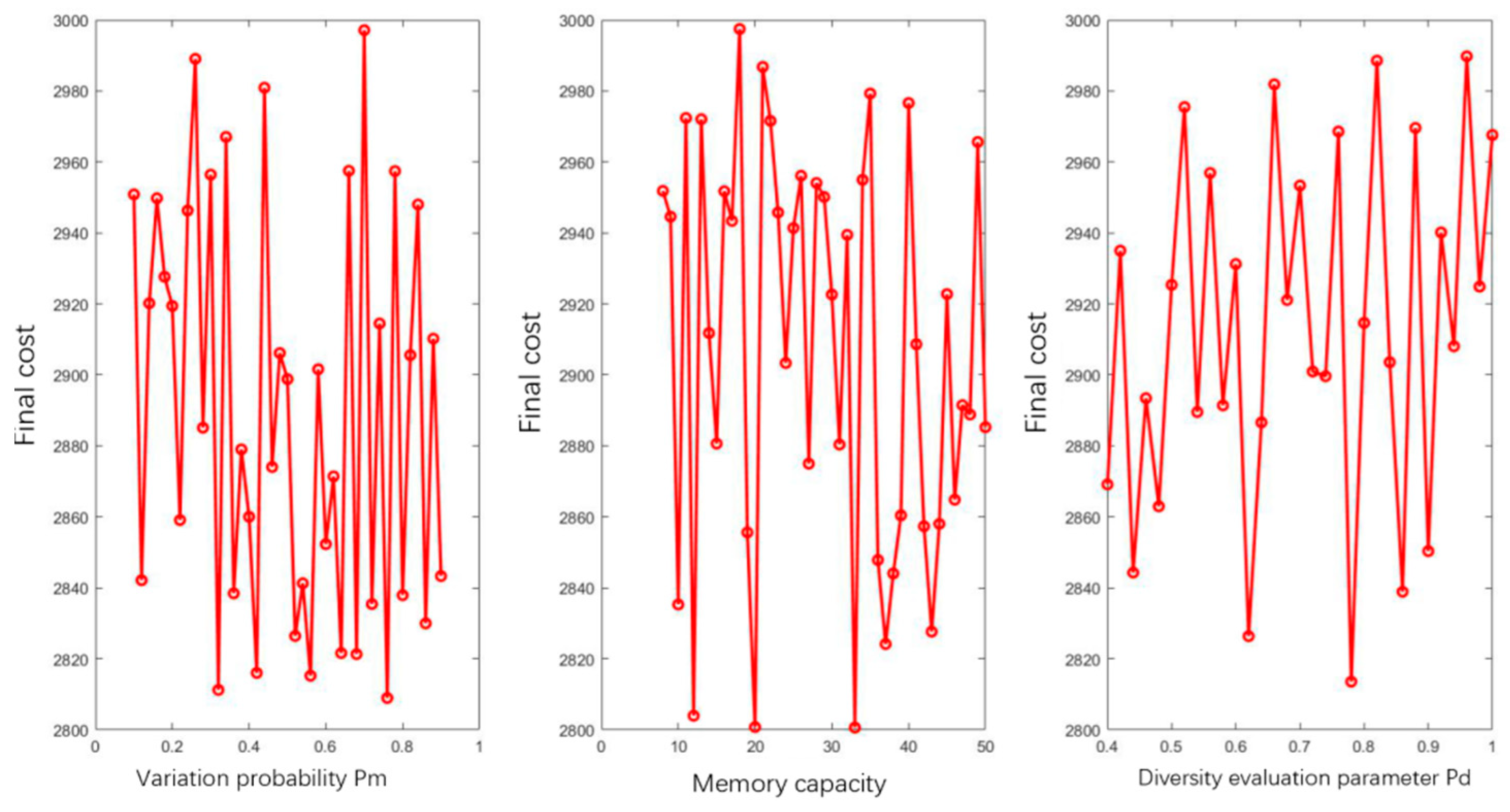
The study performs sensitivity analyses on three types of parameters: memory pool capacity, diversity evaluation parameter, and mutation probability, to assess their impact on the DPAIA algorithm’s solution for the stop location problem. Over 40 sets of parameter values are selected for each of these parameters in ranges varying from 0 to 1 for the mutation probability, 0 to 50 for the memory pool capacity, and 0.4 to 1 for the diversity evaluation parameter. Using the method of controlled variables, the convergence costs under different parameters are calculated, and the results are illustrated in Figure 4.
In Figure 4, the horizontal axis represents the variation range of different parameters, and the vertical axis represents the convergence cost for solving the model. It can be seen that the optimal convergence cost varies under different parameters. For each experimental group, the best parameter values corresponding to the lowest convergence cost are chosen as the algorithm parameters. The lowest cost of 2809 occurs when the mutation probability Pm is 0.76, the lowest cost of 2802 is achieved when the memory pool capacity C is 33, and the lowest cost of 2814 is reached when the diversity evaluation parameter Pd is 0.78. Hence, the optimal configuration of the DPAIA algorithm parameters is determined as Pm = 0.76, C = 33, and Pd = 0.78.
The parameter calibrations for the improved DBSCAN clustering algorithm and the improved AP clustering algorithm mainly refer to the parameter values in the authors’ experiments. The calibrated parameter results are summarized in Table 3.

5.2.2. Evaluation Indicator Settings

The selection rate of customized buses is influenced by the walking distance for passengers, and several scholars have conducted related studies on this issue [13]. Optimizing stop positions can change the travel distance and thus affect passengers’ mode choice. However, in actual operations, besides considering walking distances, operators of customized buses must consider the economic costs of operating such services. The core issue in custom bus operation is how to increase operator profitability while meeting passenger travel needs [10,14]. This study transforms passenger walking distances into economic costs and establishes the following evaluation indicator, considering both the economic cost of establishing stops for the operator:
A = r v i p T + n L o
where r v i p T is the total annual passenger travel cost, r is the average daily walking distance for passengers, i is the number of demand points within a year, p is the per capita disposable income in Chengdu for 2021 (CNY/year), T is the total annual working time in seconds for laborers in Chengdu, n is the total number of established bus stops, L is the cost of constructing a single bus stop, and o is the average lifespan of a bus stop.
Based on research findings, p = 45,755 CNY/year, T = 22,550,400 s, v = 1.1 m/s, o = 8 years, L = CNY 30,000, and, hence, A = 199.2r + 3750n.

5.2.3. Solving the Customized Bus Stop Location Problem

This section uses the Improved DBSCAN Clustering Algorithm, the Improved AP Clustering Algorithm, and the IA Algorithm and the DPAIA Algorithm proposed in this paper to solve the customized bus stop location model established in Section 3, subsequently obtaining the stop locations and conducting a comparative analysis of the solutions [15,16].
(1)
Utilizing Enhanced DBSCAN for Bus Stop Clustering
When applying the DBSCAN clustering algorithm, the cluster discrimination method proposed by the author is used to identify noise points by calculating dispersion degrees. Demand points with high dispersion are classified as noise, and those in the urban center are grouped into different clusters. Subsequently, noise points are removed, and the remaining demand point data are divided into 35 clusters according to their categories. Finally, through the author’s proposed evaluation indicator, it is determined whether additional stops are needed. The application of the Improved DBSCAN Clustering Algorithm concludes that 41 bus stops are required, with an average daily walking distance of 731 m for passengers.
(2)
Using Improved AP Clustering Algorithm for Platforms
During the application of the AP clustering algorithm, no pre-set number of stops is necessary to obtain an effective stop layout. By introducing a similarity adjustment factor based on the AP clustering algorithm, the algorithm increases the similarity value between nodes, balances the importance among cluster centers, and raises the likelihood of selected nodes becoming cluster centers. This leads to shared-ride station planning that caters to the majority of passengers’ preferences and travel distances. The Improved AP Clustering Algorithm determines that 39 bus stops are needed, with an average daily walking distance of 737.4 m for passengers.
(3)
Using IA algorithm and DPAIA algorithm to solve the model
Considering both economic costs and customer satisfaction, this paper constructs a customized bus stop location model in Chapter 3. In this chapter, based on the Matlab R2021a environment and parameters mentioned above, the model is solved using both the IA Algorithm and the DPAIA Algorithm proposed in this paper.
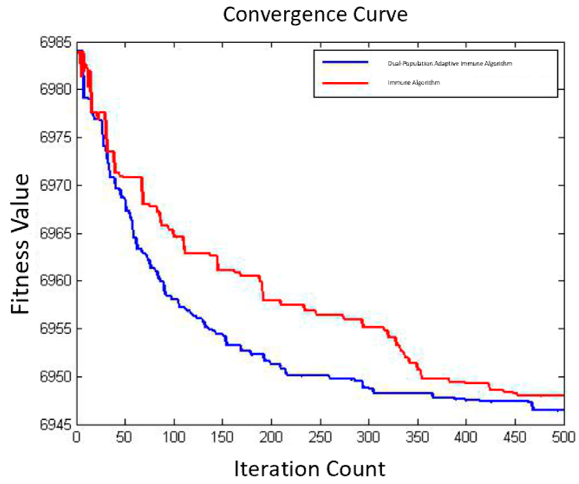
The iterative curve of the optimal fitness value for the customized bus stop location model using the IA algorithm and DPAIA algorithm is shown in Figure 5. The horizontal axis represents the number of iterations, the vertical axis represents the fitness value, the red solid line represents the iterative curve of the optimal fitness value solved by the DPAIA algorithm, and the blue solid line represents the iterative curve of the optimal fitness value solved by the IA algorithm. In the early stages of algorithm operation, the fitness of the two algorithms decreases significantly, reflecting the fast convergence speed and strong global search ability of the algorithms; with continuous iteration calculation, the DPAIA algorithm reaches convergence when the number of iterations is 450. Finally, the IA algorithm was used to solve the model, resulting in a total of 50 platforms and an average daily travel distance of 689 m for passengers; using the DPAIA algorithm to solve the model, it was found that there are a total of 50 platforms, and the average daily travel distance of passengers is 512 m. Compared to the IA algorithm, the DPAIA algorithm proposed in this paper has better solving ability. The DPAIA algorithm introduces foreign invasive populations and sets adaptive mutation rate and crossover rate during model solving, making the algorithm converge faster and the solution results better. This indicates that the DPAIA algorithm proposed in this paper is more reasonable in solving the bus stop location model, and the final solved station position better meets customer needs and the long-term interests of the company.

5.3. Comparison and Analysis of Experimental Results

To demonstrate the effectiveness of the proposed model and algorithms, this study conducts a quantitative analysis of the bus stop location solutions obtained using the four methods, as shown in Table 4.
From Table 4, it can be deduced that the weighted cost of the solution found by the DPAIA algorithm is the smallest at CNY 28.95 ten thousand. Although the DPAIA solution requires nine more bus stations than the Improved DBSCAN Clustering Algorithm and eleven more than the Improved AP Clustering Algorithm, which marginally increases the company’s economic costs, its optimized bus stop layout significantly reduces passengers’ daily walking distance, thereby lowering their walking distance costs. This improvement encourages more residents to choose customized buses during their daily commutes, potentially alleviating traffic congestion in the city. The increased passenger preference will likely lead to higher profits for the company.

5.4. Customized Bus Stop Location Results

Upon comparing the experimental results, it was discovered that the bus stop location scheme derived from the DPAIA algorithm has the overall lowest cost, making it the preferred solution for the final bus stop locations. Consequently, the model suggests a total of 50 customized bus stations. Their coordinates and covered passenger groups are detailed in Table 5. Longitude and latitude denote the geographical coordinates of each bus stop, while CAP indicates the number of passenger groups served. Placing the passenger demand points and the derived bus stop locations onto the road network generates a map of the customized bus stop locations. The result from the DPAIA algorithm is depicted in Figure 6, where red square markers represent the bus stop positions and green circular markers represent the passenger positions. The figure illustrates that the bus stop positions are distributed logically, aligning well with the demand points and situated along the road network, fulfilling the practical requirements for building bus stops.

6. Conclusions

In this paper, we tackled the problem of customized bus stop location by developing a novel model based on the immune algorithm. Our approach integrates “data analysis + mathematical modeling + solution” to achieve a balanced outcome that addresses the needs of both passengers and operators. Specifically, we introduced the Dual Population Adaptive Immunity Algorithm (DPAIA) to solve this model. By enhancing the traditional immune algorithm with adaptive crossover and mutation rates, we effectively reduced computational costs. Additionally, the introduction of an invading population, which is periodically combined with the main population, ensured diversity and prevented the algorithm from converging prematurely on local optima. Our results demonstrate that the DPAIA successfully identifies bus stop locations that minimize the weighted sum of passengers’ walking distances and the operator’s economic expenditures, offering a robust solution to the customized bus stop location problem.

Author Contributions

Conceptualization, T.Y., H.L. and Y.W. (Yawen Wang); methodology, H.L. and Y.W. (Yawen Wang); software, F.Y. and Q.G.; validation, F.Y. and Q.G.; data curation, T.Y.; writing—original draft preparation, Y.W. (Yawen Wang); writing—review and editing, T.Y. and Y.W. (Yizeng Wang). All authors have read and agreed to the published version of the manuscript.

Funding

This research received no external funding.

Data Availability Statement

The authors will supply the relevant data in response to reasonable requests.

Conflicts of Interest

The authors declare no conflict of interest.

References

  1. Huang, K.; Xu, L.; Chen, Y.; Cheng, Q.; An, K. Customized Bus Route Optimization with the Real-Time Data. J. Adv. Transp. 2020, 2020, 1–9. [Google Scholar] [CrossRef]
  2. Chen, F.; Peng, H.; Ding, W.; Ma, X.; Tang, D.; Ye, Y. Customized bus passenger boarding and deboarding planning optimization model with the least number of contacts between passengers during COVID-19. Phys. A Stat. Mech. Its Appl. 2021, 582, 126244. [Google Scholar] [CrossRef] [PubMed]
  3. Huo, E.; Mu, R.; Luan, S. Research on Customized Bus Stop Site Selection Based on Online Ride hailing Data. In Proceedings of the World Transportation Congress, Bombay, India, 26–31 May 2019. [Google Scholar]
  4. Xue, H.; Wang, J. Research on two-step optimization site selection method for customized bus sharing stations. Transp. Technol. Econ. 2015, 23, 14–19. [Google Scholar]
  5. Wang, W.; Wang, Q.; Guo, M. Design of Urban Customized Bus Routes and Platforms. Chin. Mark. 2019, 27, 120–121. [Google Scholar]
  6. Liu, C.; Liu, K. Research on Customized Bus Route and Platform Design; Dalian University of Technology: Dalian, China, 2019. [Google Scholar]
  7. Kumar, K.M.; Rama Mohan Reddy, A. A fast DBSCAN clustering algorithm by accelerating neighbor searching using Groups method. Pattern Recognit. 2016, 58, 39–48. [Google Scholar] [CrossRef]
  8. Liu, Q.; Chen, M. Research on Customized Bus Stop Site Selection and Route Planning Based on Taxi Demand; Chongqing Jiaotong University: Chongqing, China, 2021. [Google Scholar]
  9. Zhang, H. Research on Customized Public Transport Route Planning Based on Granular Computing; Hangzhou University of Electronic Science and Technology: Sichuan, China, 2019. [Google Scholar]
  10. Sun, Y. Research on Customized Bus Stop Site Selection and Route Design Method Based on Platform Demand Data; Beijing Jiaotong University: Beijing, China, 2019. [Google Scholar]
  11. Wenjia, S.; Hongmei, S.; Di, D. Research on Cold Chain Logistics Distribution Paths Based on Optimized Immune Algorithm. Appl. Microcomput. 2019, 35, 103–107. [Google Scholar]
  12. Zhou, Y. Optimization of Urban Passenger Transport Structure Based on Generalized Travel Costs; Southwest Jiaotong University: Sichuan, China, 2020. [Google Scholar]
  13. Wang, J.; Yamamoto, T.; Liu, K. Role of customized bus servbices in the transportation system: Insight from actual performance. J. Adv. Transp. 2019, 5, 1–14. [Google Scholar] [CrossRef]
  14. Song, H.; Gao, S.; Li, Y.; Liu, L.; Dong, H. Train-Centric Communication Based Autonomous Train Control System. IEEE Trans. Intell. Veh. 2023, 8, 721–731. [Google Scholar] [CrossRef]
  15. Wu, W.; Song, H.; Wang, H.; Dong, H. Potential Game Based Task Offloading in the High-Speed Railway with Reinforcement Learning. IEEE Trans. Intell. Transp. Syst. 2023, 24, 12671–12685. [Google Scholar] [CrossRef]
  16. Song, H.; Li, L.; Li, Y.; Tan, L.; Dong, H. Functional Safety and Performance Analysis of Autonomous Route Management for Autonomous Train Control System. IEEE Trans. Intell. Transp. Syst. 2024, 1–14. [Google Scholar] [CrossRef]
Figure 1. Flowchart of the DPAIA algorithm.
Mathematics 12 02382 g001
Figure 2. Ride-hailing demands at different times.
Mathematics 12 02382 g002
Figure 3. Distribution map of custom bus passenger demands.
Mathematics 12 02382 g003
Figure 4. Convergence costs under different parameters.
Mathematics 12 02382 g004
Figure 5. Comparison of convergence curves before and after improvement.
Mathematics 12 02382 g005
Figure 6. DPAIA algorithm’s bus stop location result.
Mathematics 12 02382 g006
Table 1. Processing of abnormal data.
Abnormal TypeData AnomalyPreprocessing Measures
Location MissingRide-hailing vehicle’s geographic location missingSupplement based on the previous time point and interval
Location AnomalyRide-hailing vehicle not within the considered interval at a certain timeSupplement based on the previous time point and interval
Data AnomalyOrigin and destination points not within the considered intervalDelete this data entry
Time MissingRide-hailing vehicle time missing at a certain timeDelete this data entry
Data DeduplicationDuplicate road dataMerge consecutive road segments if the cosine of the angle θ between them is greater than 0.9848
Table 2. Model Parameters.
Parameter TypeSymbolMeaningValue
Model ParametergWalking Distance Cost per Passenger (CNY/m)0.002
RMaximum Walking Distance to the Stop (m)1000
lConstruction Cost per Stop (CNY 10,000)3
NmaxMaximum Number of Stops100
NminMinimum Number of Stops20
Table 3. Algorithm parameters.
Parameter TypeSymbolMeaningValue
DPAIA AlgorithmPopsizeInitial Population Size50
CMemory Pool Capacity33
iterNumber of Iterations100
PCCrossover Probability0.5
PmMutation Probability0.76
pdDiversity Evaluation Parameter0.78
Improved DBSCAN ClusteringEPsNeighborhood Radius in Dense Regions300
minPtsThreshold for Core Points3
Improved AP ClusteringpReference Degree Value−51,465
dmWeight of Central Node7
dWeight of Other Nodes1
Table 4. Comparison of solutions from four algorithms.
IDAlgorithmr (m)n (Unit)A (CNY 10,000)
1Improved DBSCAN Clustering Algorithm7314129.94
2Improved AP Clustering Algorithm7373929.30
3IA Algorithm6895032.47
4DPAIA Algorithm5125028.95
Table 5. Coordinates and covered passenger groups of bus stations.
IDLongitudeLatitudeCAPIDLongitudeLatitudeCAP
1104.08526630.64744226104.0224830.6651628
2104.07463930.67136827104.07865730.6554438
3104.03864930.64032628104.08573830.673013
4104.04394330.67384529104.07093530.6434568
5104.0600430.6694630104.09376830.6458557
6104.07526630.66889731104.02707830.6531813
7104.07490730.62563732104.05029130.667094
8104.06762830.65542533104.07065430.6450895
9104.08396830.64107534104.04557730.6529668
10104.06143230.66351535104.06649630.646044
11104.02141630.63958736104.06039730.6386918
12104.07422430.67425437104.06246930.6765716
13104.07157830.69363638104.08982230.6316296
14104.03208930.66554639104.05165730.691759
15104.10638930.67425840104.03113830.6565364
16104.09294930.64713341104.07859930.665274
17104.06394330.62159242104.09228530.6553843
18104.07833430.6629943104.09518330.68044313
19104.04773630.66235844104.05242330.653044
20104.07963330.63328845104.09064630.6575837
21104.0875330.66646446104.04155130.6393717
22104.09618530.65867447104.08086530.6562615
23104.087830.68394748104.09752230.6785799
24104.06246330.68097849104.05080730.6357315
25104.08114330.66281650104.08398430.6486926
Disclaimer/Publisher’s Note: The statements, opinions and data contained in all publications are solely those of the individual author(s) and contributor(s) and not of MDPI and/or the editor(s). MDPI and/or the editor(s) disclaim responsibility for any injury to people or property resulting from any ideas, methods, instructions or products referred to in the content.