Spatial Durbin Model with Expansion Using Casetti’s Approach: A Case Study for Rainfall Prediction in Java Island, Indonesia

Abstract

Research on rainfall is critically important due to its significant impact on climate change and natural disasters in Indonesia. Various factors influence rainfall variability. Consequently, when examining spatial aspects, it is likely that spatial dependency exists not only in the response variable but also in the exogenous variables. Hence, a model that accounts for spatial dependencies between these variables is required. The integration of the Spatial Durbin Model (SDM) with Casetti’s expansion approach can be utilized to predict spatial patterns of rainfall influenced by exogenous variables. By incorporating spatial effects and relevant independent variables, this model can provide more precise estimates of rainfall distribution across different regions. This modeling technique is particularly effective for accurate rainfall prediction, considering exogenous factors such as air temperature, humidity, solar irradiation, and surface pressure. The SDM with Casetti’s expansion approach was employed to predict rainfall patterns in the Java Island region, utilizing data from the National Aeronautics and Space Administration’s Prediction of Worldwide Energy Resources (NASA POWER) big data website. The application of this model in the context of rainfall prediction highlights its importance in enhancing the understanding of weather dynamics and aiding disaster risk mitigation in Java Island, a highly populated region characterized by a Monsoon rainfall pattern. The rainfall prediction follows a Knowledge Discovery in Databases (KDD) methodology. The results of this study are expected to be valuable to relevant agencies, such as the Meteorology, Climatology, and Geophysics Agency (BMKG), and agribusiness companies, improving agricultural planning and planting seasons. Additionally, the general public can benefit from more accurate climate information, particularly regarding rainfall. The computational framework is developed within an RShiny web application, and the performance of the proposed technique is measured by the Mean Absolute Percentage Error (MAPE), achieving a very accurate prediction rate of 2.78%.

1. Introduction

Indonesia, a tropical archipelago, experiences high rainfall throughout the year. This is primarily due to its location around the equator and its geographical position between the Asian and Australian continents, as well as the Pacific and Indian Oceans [1]. Research on rainfall is critically important because this phenomenon significantly affects various aspects of human life and the environment, including agriculture, public health, water resource management, climate change, and natural disasters. Extreme rainfall can lead to natural disasters such as floods, landslides, and flash floods [2]. In October 2023, 41.16% of Indonesia experienced low-category rainfall, 49.05% experienced medium-category rainfall, and 9.79% experienced high- to very high-category rainfall. Out of 4879 observation points, 21 stations recorded extreme rainfall exceeding 150 mm/day [3]. Indonesia exhibits three distinct rainfall patterns: monsoon, equatorial, and local [4,5,6,7]. The Meteorology, Climatology, and Geophysics Agency (BMKG) of Indonesia categorizes the country’s regions based on these rainfall patterns, as shown in Figure 1 [8]. The monsoonal pattern is primarily influenced by monsoon circulation, which changes direction every six months, resulting in one peak during the rainy season and another during the dry season. The monsoonal rainfall pattern, characterized by a unimodal distribution (one peak), brings the rainy season from December to February (DJF) and the dry season from June to August (JJA), with a single peak during the rainy season. Regions with monsoonal rainfall patterns include eastern and southern Sumatra, Java, Bali, the Nusa Tenggara islands, southern Kalimantan, the west coast of South Sulawesi, the west coast of Southeast Sulawesi, the Buton and Muna islands, northern Sulawesi, southern Maluku, and the northern coast of Papua, including Merauke. On the other hand, areas with the equatorial rainfall pattern experience a bimodal distribution, with two peaks of maximum rainfall, and almost the entire year falls under the rainy season criteria. The equatorial pattern exhibits a semi-monsoonal rhythm with two distinct peaks in the rainy season, typically occurring around March and October. Regions characterized by equatorial rainfall patterns include western Sumatra, northern Kalimantan, parts of Central Sulawesi and South Sulawesi (Luwu Raya and Toraja regions), and central Papua. Conversely, the local pattern contrasts with the monsoonal type by featuring a unimodal rainfall pattern, but with characteristics distinct from monsoonal rainfall. Areas exhibiting local rainfall patterns include Parigi Moutong, Palu, Luwuk Banggai, the Banggai Islands, Taliabu, Sula, southern Buru, southern Seram, Ambon, Sorong, Raja Ampat, Teluk Bintuni, Fak-fak, and the eastern coast of South Sulawesi. Indonesia experiences relatively high average rainfall, ranging from 2000 to 3000 mm per year, making it an important subject for study. This research focuses on Java Island, which exhibits a monsoonal rainfall pattern.

Understanding rainfall patterns is crucial for guiding strategic planning and enhancing resilience across relevant sectors or agencies to mitigate climate variability and natural disasters. These patterns are integral to achieving Sustainable Development Goal (SDG) 13, which emphasizes ‘Climate Action’ and calls for urgent measures to mitigate and adapt to climate change [9]. A thorough understanding and effective management of rainfall patterns are essential for advancing SDG 13 objectives. This includes addressing the impacts of changing rainfall patterns on various sectors, strengthening resilience against extreme weather events, and promoting sustainable practices in water and land management.

Spatial modeling typically involves the development of mathematical or computational frameworks to depict spatial relationships or patterns within data [10]. These models are extensively employed across various disciplines to analyze spatial dimensions and phenomena [11]. Literature has shown that the application of spatial models is instrumental in the prediction of rainfall and climate dynamics. Over recent decades, spatial modeling has advanced through diverse methodological approaches. For instance, Triyatno et al. (2023) utilized a hybrid spatial model to assess flood hazards in the Tarusan Watershed, projecting significant changes from 2019 to 2039 [12]. In another study, Bonsoms et al. (2023) compared the performance and accuracy of traditional linear methods (Multiple Linear Regression and Generalized Additive Models) with five machine learning techniques (K-Nearest Neighbors, Support Vector Machines, Neural Networks, Stochastic Gradient Boosting, and Random Forest) for spatial interpolation of climatological variables in a mountainous region [13]. Anna et al. (2021) developed a spatial model using the rational modification method to mitigate local flooding hazards in Surakarta, Indonesia [14]. Jalbert et al. (2022) applied a Bayesian hierarchical model to interpolate precipitation extremes parameters across a large spatial domain, facilitating IDF curve construction at unmonitored locations [15]. Falah et al. (2023) employed a hybrid Spatial Autoregressive Exogenous (SAR-X) model approach, integrating Casetti’s method, to predict rainfall patterns in West Java, Indonesia [16].

Rainfall interacts with various climate variables such as air temperature, humidity, solar irradiation, and surface pressure, all of which exhibit regional variability [17]. In the context of spatial modeling, the heterogeneity in the SAR-X model is used to describe different parameter values for each spatial observation through the distance between locations [16]. However, a limitation of the SAR-X model is its focus solely on spatial dependence of the response variable, neglecting potential spatial relationships among exogenous variables. In the context of spatial modeling, it is crucial to consider spatial dependencies across both response and exogenous variables. To address this issue, the Spatial Durbin Model (SDM) is proposed in this study; this model is specifically designed to account for spatial interdependencies among both response and exogenous variables [18]. Furthermore, the SDM is enhanced through the expansion using the Casetti approach, which refines parameter estimation across spatial observations [19]. This dual modeling approach aims to provide a more comprehensive understanding of spatial dependencies in the context of rainfall prediction and climate modeling.

By integrating spatial effects and relevant independent variables, the model enhances the precision of rainfall distribution estimates across different regions. The Spatial Durbin Model (SDM) with expansion using Casetti’s approach offers several advantages. Firstly, it facilitates the identification of spatial rainfall patterns, capturing spatial dependencies among observation units within the region. Secondly, through the incorporation of pertinent exogenous variables, the model improves the accuracy of rainfall predictions. Thirdly, the results from the model can support disaster mitigation, water resources management, and resilient infrastructure development against natural disasters. This study explores the application of the SDM with expansion using Casetti’s approach in rainfall prediction, highlighting its significance in advancing understanding of weather dynamics and bolstering disaster risk mitigation, particularly in densely populated regions like Java Island. The research employs an integrated R script developed for the SDM with expansion using Casetti’s approach, implemented through the RShiny version 1.7.4 web application to optimize the prediction process.

2. Materials and Methods

2.1. Inverse Distance Weight Matrix

A matrix that expresses the proximity relationship between locations is called a spatial weight matrix. In this study, the distance weight, also known as the inverse distance weight matrix, is used to represent the true distance between sites. The latitude and longitude of the observed location’s center point are used to determine the distance between two locations. We denote well-defined location coordinates as $x_{ij}\left(u_{ij},v_{ij}\right)$ for location i and j, with $i,j=\mathrm{1,2},3\dots ,N$ locations, while u_ij and v_ij indicate the latitude and longitude coordinates of the ith and jth location. The Euclidean distance is used to measure, $d_{ij}$, the distance between location i and location $j$ [20], as follows:

$$d_{ij}=\sqrt{{\left(x_i\left(u_i\right)-x_j\left(u_j\right)\right)}^2+{\left(x_i\left(v_i\right)-x_j\left(v_j\right)\right)}^2},$$

(1)

where

• $u_i$ is the latitude of the $i\mathrm{th}$ location, $i=1,2,3,\mathrm{\dots },N$,
• $v_i$ is the longitude $i\mathrm{th}$ location,
• $u_j$ is the latitude of the jth location, j = 1, 2, 3, …, N, and
• $v_j$ is the longitude of the $j\mathrm{th}$ location.

The Euclidean distance calculations are converted to kilometers using a conversion factor of 111.319, that is, $\left|d_{ij}\right|\times 111.319$. This conversion factor corresponds to the distance represented by one degree of longitude [21]. The actual distance between observation locations is then weighted as the inverse distance, computed using the following equation [22]:

$$w_{ij}=\left\{\begin{array}{cc}{\displaystyle \frac{1}{d_{ij}}},& i\ne j\\ 0,& i=j\end{array}\right..$$

(2)

Next, if the sum of the distance weights of a row in the inverse distance weight matrix is not equal to 1 then the distance weights must be standardized [23] to obtain ${\displaystyle \sum _{j=1}^N{w}_{ij}=1}, \forall i=1,2,3,\dots ,N,$ where:

$$w_{ij}^{*}={\displaystyle \frac{w_{ij}}{{\sum }_{j=1}^N{w}_{ij}}}, \forall i=\mathrm{1,2},3,\dots ,N.$$

(3)

2.2. Moran Index

One approach to determine the presence of spatial dependencies and check the spatial relationship or correlation between locations is to conduct a spatial autocorrelation test using the Moran Index statistic. Spatial autocorrelation is an estimate of the correlation between observation values associated with locations on the same variable. If there is a systematic pattern in the distribution of a variable, then there is spatial autocorrelation. Spatial autocorrelation explains the dependency of spatial data between one location and another based on a measure of proximity or intersection [18].

$$I={\displaystyle \frac{n{\displaystyle \sum _{i=1}^n{\displaystyle \sum _{j=1}^n{w}_{ij}\left(x_i-\overline{x}\right)\left(x_j-\overline{x}\right)}}}{{\displaystyle \sum _{i=1}^n{\displaystyle \sum _{j=1}^n{w}_{ij}}}{\displaystyle \sum _{i=1}^n{\left(x_i-\overline{x}\right)}^2}}}.$$

(4)

The hypothesis formulation in this test is as follows:

• $H_0:I=I_0$ There is no spatial autocorrelation between locations, vs.
• $H_1:I\ne I_0$ There is spatial autocorrelation between locations,
• With $I_0=E(I)$.

The test statistic employed is expressed below:

$$Z\left(I\right)={\displaystyle \frac{I-E\left(I\right)}{\sqrt{Var\left(I\right)}}}\sim N\left(0,1\right),$$

(5)

with

$$E\left(I\right)=-{\displaystyle \frac{1}{n-1}},$$

(6)

$$Var\left(I\right)={\displaystyle \frac{n^2{S}_1-n{S}_2+3S_0^2}{\left(n^2-1\right)S_0^2}}-{\left[E\left(I\right)\right]}^2,$$

(7)

$$S_0={\displaystyle \sum _{i=1}^n{\displaystyle \sum _{j=1}^n{w}_{ij}}},\hspace{1em}\hspace{1em}{S}_1={\displaystyle \frac{1}{2}}{\displaystyle \sum _{1\ne j}^n{\left(w_{ij}+w_{ji}\right)}^2},\hspace{1em}\hspace{1em}{S}_2={{\displaystyle \sum _{i\ne j}^n\left({\displaystyle \sum _{i=1}^n{w}_{ij}+{\displaystyle \sum _{j=1}^n{w}_{ji}}}\right)}}^2$$

where

• $I$ is the Moran Index value,
• $n$ is the number of observation locations,
• $x_i$ is the value of the observation variable at the ith location,
• $x_j$ is the value of the observation variable at jth location,
• $\overline{x}$ is the average of the number of variables, and
• $w_{ij}$ is an element of the standardized weight matrix between locations $i$ and $j$.

The Moran Index ranges between [−1, 1]. A negative value indicates negative spatial autocorrelation, while a positive value signifies positive spatial autocorrelation [24]. We observe from Equation (6) that as the number of spatial locations increases, the expected value E(I) = E₀ moves closer to zero, indicating that the expected level of spatial autocorrelation under the null hypothesis (no spatial autocorrelation) diminishes as the number of observation locations increases. On the other hand, it becomes more negative with fewer spatial observation locations, indicating a greater expected negative spatial autocorrelation under the null hypothesis.

• Decision Rule:

The null hypothesis is rejected based on the following decision rule:

$$\mathrm{Reject} H_0 \mathrm{at} \mathrm{the} \mathrm{significance} \mathrm{level} \alpha \mathrm{if} -Z_{score}\le -Z_{\raisebox{1ex}{$\alpha $}\!\left/ \!\raisebox{-1ex}{$2$}\right.} \mathrm{or} Z_{score}\ge Z_{\raisebox{1ex}{$\alpha $}\!\left/ \!\raisebox{-1ex}{$2$}\right.}.$$

2.3. Spatial Durbin Model

The Spatial Durbin Model (SDM) is a spatial regression model similar to the Spatial Autoregressive (SAR) model, featuring a spatial lag in the response variable. However, unlike the SAR model, the SDM is distinguished by incorporating a spatial lag in the exogenous variables [18]. According to [25], the SDM is described as follows

$$\mathit{y}=\rho \mathbf{W}\mathit{y}+\alpha {\mathbf{1}}_n+\tilde{\mathbf{X}}\mathit{\beta }+\mathbf{W}\tilde{\mathbf{X}}\mathit{\theta }+\mathit{\epsilon }\mathrm{with}\mathit{\epsilon }\stackrel{iid}{\sim }N(0,{\sigma }^2\mathbf{I}),$$

(8)

or it can be written as follows:

$$\begin{gathered} y_i=\rho {\displaystyle \sum _{j=1}^n{w}_{ij}}{y}_j+\alpha +{\displaystyle \sum _{k=1}^p{\beta }_k}{x}_{ik}+{\displaystyle \sum _{k=1}^p{\displaystyle \sum _{j=1}^n{\mathit{\theta }}_k}}\left(w_{ij}{x}_{kj}\right)+{\epsilon }_i, \\ \mathit{y}=\rho \mathbf{W}\mathit{y}+\mathbf{P}\mathit{\delta }+\mathit{\epsilon }, \end{gathered}$$

(9)

where

• $\mathit{y}$ is the vector of dependent variables of size (n × 1),
• $\tilde{\mathbf{X}}$ is the matrix of independent variables of size (n × k),
• $\mathbf{P}$ = $\left[\begin{array}{ccc}{\mathbf{1}}_n& \tilde{\mathbf{X}}& \mathbf{W}\tilde{\mathbf{X}}\end{array}\right]$,
• $\mathit{\delta }$ = $\left[\begin{array}{c}\alpha \\ \mathit{\beta }\\ \mathit{\theta }\end{array}\right]$,
• $\rho$ is the spatial lag coefficient of the dependent variable,
• $\alpha$ is the constant parameter,
• $\mathit{\beta }$ is the vector of regression parameters of size (k × 1),
• $\mathit{\theta }$ is the spatial lag parameter vector of covariate variable of size (k × 1),
• $\mathbf{W}$ is the spatial weight matrix of size (n × n), and
• $\mathit{\epsilon }$ is the error vector of size (n × 1).

2.4. Spatial Expansion with Casetti’s Approach

The Spatial Expansion Model (Casetti, 1972) [19] introduced in this study addresses spatial heterogeneity by accounting for varying parameter values across spatial observations, determined by the Euclidean distance between locations based on their coordinates. The spatial expansion using Casetti’s approach, adopting a linear regression approach, is formulated as follows:

$$\begin{gathered} y=X\beta +\epsilon \mathrm{with} \epsilon \stackrel{iid}{{\displaystyle \sim }}N(0,{\sigma }^{2}I), \\ \beta =ZJ{\beta }_0, \end{gathered}$$

(10)

where

• $y$ is the vector of dependent variables of size $\left(n\times 1\right)$.
• $X$ is the matrix of independent variables of size $\left(n\times nk\right)$.
• $Z$ is the location information that contains elements $Z_{xi},Z_{yi} \mathrm{with} i=1,\dots ,n$ representing the latitude and longitude of each observation, of size $\left(nk\times 2nk\right)$.
• $J$ is the expansion of the identity matrix of size $\left(2nk\times 2k\right)$.
• $\beta$ is the matrix of size $\left(nk\times 1\right)$ contains parameter estimators for all explanatory $k$ variables at each observation.
• ${\beta }_0$ is the parameter expressed by ${\beta }_{latitude},{\beta }_{longitude}$ of size $\left(2k\times 1\right)$.
• $\otimes$ is the Kronecker product.
• $\epsilon$ is the error vector of size $\left(n\times 1\right)$.
• $s_i$ is the location matrix with $i=1,\dots ,n$.

The matrix form of the model can be written as follows:

$$\begin{gathered} y=\left(\begin{array}{c}y\left(s_1\right)\\ \begin{array}{l}y\left(s_2\right)\\ ⋮\end{array}\\ y\left(s_n\right)\end{array}\right), X=\left(\begin{array}{cccccccccc}{x}_{11}& \cdots & x_{1k}& 0& \cdots & 0& \cdots & 0& \cdots & 0\\ 0& \cdots & 0& x_{21}& \cdots & x_{2k}& 0& ⋮& \cdots & ⋮\\ ⋮& \ddots & ⋮& 0& \ddots & 0& \ddots & 0& \ddots & 0\\ 0& \cdots & 0& 0& \cdots & 0& 0& x_{n1}& \cdots & x_{nk}\end{array}\right), \\ \beta =\left(\begin{array}{c}{\beta }_1\left(s_1\right)\\ {\beta }_1\left(s_2\right)\\ ⋮\\ {\beta }_k\left(s_n\right)\end{array}\right), \epsilon =\left(\begin{array}{c}\epsilon \left(s_1\right)\\ \begin{array}{l}\epsilon \left(s_2\right)\\ ⋮\end{array}\\ \epsilon \left(s_n\right)\end{array}\right), {\beta }_0=\left(\begin{array}{c}{\beta }_{latitude}\\ {\beta }_{longitude}\end{array}\right) \\ Z=\left(\begin{array}{cccccc}{Z}_{x1}\otimes I_k& Z_{y1}\otimes I_k& 0& 0& 0& 0\\ 0& 0& \ddots & \ddots & 0& 0\\ 0& 0& 0& 0& Z_{xn}\otimes I_k& Z_{yn}\otimes I_k\end{array}\right), J=\left(\begin{array}{cc}{I}_k& 0\\ 0& I_k\\ ⋮& ⋮\\ 0& I_k\end{array}\right). \end{gathered}$$

2.5. Spatial Durbin Model with Expansion Using Casetti’s Approach

By integrating the use of SDM with expansion using Casetti’s approach, replace Equation (10) to Equation (8), to obtain the following:

$$\mathit{y}=\rho \mathbf{W}\mathit{y}+\alpha {\mathbf{1}}_n+\mathbf{X}\mathbf{Z}\mathbf{J}{\mathit{\beta }}_0+\mathbf{W}\tilde{\mathbf{X}}\mathit{\theta }+\mathit{\epsilon }\mathrm{with}\mathit{\epsilon }\stackrel{iid}{\sim }N(0,{\sigma }^{2}I).$$

(11)

Letting $\mathbf{A}=\mathbf{X}\mathbf{Z}\mathbf{J}$, it follows that:

$$\mathit{y}=\rho \mathbf{W}\mathit{y}+\alpha {\mathbf{1}}_n+\mathbf{A}{\mathit{\beta }}_0+\mathbf{W}\tilde{\mathbf{X}}\mathit{\theta }+\mathit{\epsilon }\mathrm{with}\mathit{\epsilon }\stackrel{iid}{\sim }N(0,{\sigma }^{2}I),$$

(12)

$$\mathit{y}=\rho \mathbf{W}\mathit{y}+\mathit{U}\mathit{\delta }+\mathit{\epsilon },$$

(13)

where

$\mathit{U}=\left[\begin{array}{ccc}{\mathbf{1}}_n& \mathbf{A}& \mathbf{W}\tilde{\mathbf{X}}\end{array}\right]$, and $\mathit{\delta }=\left[\begin{array}{c}\alpha \\ {\mathit{\beta }}_0\\ \mathit{\theta }\end{array}\right]$.

2.6. Parameter Estimation

The random error variable in the SDM with Expansion using Casetti’s approach is assumed to follow a normal distribution. Consequently, parameter estimation in this model adopts the SAR-X estimation method, employing the Maximum Likelihood Estimation (MLE) technique [16]. Notable sources contributing to this approach include Ord [26], Smirnov and Anselin [27], Robinson and Rossi [28], and Feng [29]. Equation (13) can be expressed as follows:

$$y=\rho Wy+\mathit{U}\mathit{\delta }+\epsilon \mathrm{with} \epsilon \stackrel{iid}{{\displaystyle \sim }}N(\mathbf{0},{\sigma }^{2}I),$$

$$\mathit{\epsilon }=\mathit{y}-\rho \mathbf{W}\mathit{y}-\mathit{U}\mathit{\delta }.$$

(14)

The probability density function used is expressed as follows:

$$f\left(y\right)={\left({\displaystyle \frac{1}{2\pi {\sigma }^2}}\right)}^{{\displaystyle \frac{n}{2}}}\exp \left[-{\displaystyle \frac{{\left(y-\rho Wy-\mathit{U}\mathit{\delta }\right)}^T\left(y-\rho Wy-\mathit{U}\mathit{\delta }\right)}{2{\sigma }^2}}\right].$$

(15)

The likelihood function of the dependent variable $y$ is formulated as follows:

$$\begin{array}{cc}L\left(\rho ,\mathit{\delta }|y\right)& =f\left(y|\rho ,\mathit{\delta }\right)\hfill \\ & ={\left({\displaystyle \frac{1}{2\pi {\sigma }^2}}\right)}^{{\displaystyle \frac{n}{2}}}\exp \left[-{\displaystyle \frac{{\left(y-\rho Wy-\mathit{U}\mathit{\delta }\right)}^T\left(y-\rho Wy-\mathit{U}\mathit{\delta }\right)}{2{\sigma }^2}}\right].\hfill \end{array}$$

(16)

Furthermore, the log-likelihood function is obtained as:

$$\begin{array}{cc}\ln L\left(\left.\rho ,\mathit{\delta }\right|\epsilon \right)& =\ln {\left({\displaystyle \frac{1}{2\pi {\sigma }^2}}\right)}^{{\displaystyle \frac{n}{2}}}\exp \left[-{\displaystyle \frac{{\left(y-\rho Wy-\mathit{U}\mathit{\delta }\right)}^T\left(y-\rho Wy-\mathit{U}\mathit{\delta }\right)}{2{\sigma }^2}}\right]\hfill \\ & =-{\displaystyle \frac{n}{2}}\ln \left(2\pi \right)-{\displaystyle \frac{n}{2}}\ln {\sigma }^2-{\displaystyle \frac{{\left(y-\rho Wy-\mathit{U}\mathit{\delta }\right)}^T\left(y-\rho Wy-\mathit{U}\mathit{\delta }\right)}{2{\sigma }^2}}.\hfill \end{array}$$

(17)

Parameter estimation of $\rho \mathrm{a}\mathrm{n}\mathrm{d} \mathit{\delta }$ are obtained by maximizing the log-likelihood function.

To obtain the maximum likelihood estimate $\widehat{\rho }$, we take the first derivative of Equation (17) with respect to $\rho$ as follows:

$$\begin{array}{cc}{\displaystyle \frac{\partial \ln L\left(\left.\rho ,\mathit{\delta }\right|\epsilon \right)}{\partial \mathit{\delta }}}& =-{\displaystyle \frac{{\left(y-\rho Wy-\mathit{U}\mathit{\delta }\right)}^T\left(-Wy\right)}{2{\sigma }^2}}\hfill \\ & ={\displaystyle \frac{{\left(y-\rho Wy-\mathit{U}\mathit{\delta }\right)}^T\left(Wy\right)}{2{\sigma }^2}},\hfill \end{array}$$

(18)

Taking ${\left.{\displaystyle \frac{\partial \ln L\left(\left.\rho ,\mathit{\delta }\right|\epsilon \right)}{\partial \rho }}\right|}_{\rho =\widehat{\rho }}$ = 0, it follows that

$${\displaystyle \frac{{\left(y-\rho Wy-\mathit{U}\mathit{\delta }\right)}^T\left(Wy\right)}{2{\sigma }^2}}=0.$$

(19)

In Equation (19), we multiply by $2{\sigma }^2{\left(Wy\right)}^T$ to obtain

$${\left(y-\rho Wy-\mathit{U}\mathit{\delta }\right)}^T\left(Wy{\left(Wy\right)}^T\right)=0.$$

(20)

Then, we multiply Equation (20) by ${\left(Wy{\left(Wy\right)}^T\right)}^{-1}$ to obtain

$${\left(y-\rho Wy-\mathit{U}\mathit{\delta }\right)}^T=0.$$

(21)

By transposing Equation (21), we obtain

$$y-\mathit{U}\mathit{\delta }=\rho Wy.$$

(22)

Multiplying both sides of Equation (22) by ${\left(Wy\right)}^T$ results in

$${\left(Wy\right)}^T\left(y-\mathit{U}\mathit{\delta }\right)={\left(Wy\right)}^T\rho Wy.$$

(23)

Furthermore, multiplying both sides of Equation (23) by ${\left({\left(Wy\right)}^{T}Wy\right)}^{-1}$ allows us to obtain

$${\left({\left(Wy\right)}^{T}Wy\right)}^{-1}{\left(Wy\right)}^T\left(y-\mathit{U}\mathit{\delta }\right)={\left({\left(Wy\right)}^{T}Wy\right)}^{-1}\left({\left(Wy\right)}^{T}Wy\right)\rho ,$$

(24)

$$\widehat{\rho }={\left({\left(Wy\right)}^{T}Wy\right)}^{-1}{\left(Wy\right)}^T\left(y-\mathit{U}\mathit{\delta }\right).$$

(25)

There is a constraint that must be applied to the parameter $\rho$. It was noted by Anselin and Florax (1994) that this parameter can have realistic values in the following range [30]:

$${\displaystyle \raisebox{1ex}{$1$}\!\left/ \!\raisebox{-1ex}{${\lambda }_{\min }$}\right.}<\rho <{\displaystyle \raisebox{1ex}{$1$}\!\left/ \!\raisebox{-1ex}{${\lambda }_{\max }$}\right.},$$

where ${\lambda }_{\min }$ represents the minimum eigenvalue of the standardized spatial contiguity matrix W and ${\lambda }_{\max }$ denotes the largest eigenvalue of this matrix. This requires that the optimization search is constrained to values of $\rho$ within the range [19].

To obtain the maximum likelihood estimate $\widehat{\mathit{\delta }}$, take the first derivative of Equation (17) with respect to $\mathit{\delta }$ as follows:

$$\begin{array}{cc}{\displaystyle \frac{\partial \ln L\left(\left.\rho ,\mathit{\delta }\right|\epsilon \right)}{\partial \mathit{\delta }}}& =-{\displaystyle \frac{{\left(y-\rho Wy-\mathit{U}\mathit{\delta }\right)}^T\left(-\mathit{U}\right)}{2{\sigma }^2}}\hfill \\ & ={\displaystyle \frac{{\left(y-\rho Wy-\mathit{U}\mathit{\delta }\right)}^T\left(\mathit{U}\right)}{2{\sigma }^2}}.\hfill \end{array}$$

(26)

Set ${\left.{\displaystyle \frac{\partial \ln L\left(\left.\rho ,\mathit{\delta }\right|\epsilon \right)}{\partial \mathit{\delta }}}\right|}_{\mathit{\delta }=\widehat{\mathit{\delta }}}=0$, to have the equation that follows:

$${\displaystyle \frac{{\left(y-\rho Wy-\mathit{U}\mathit{\delta }\right)}^T\mathit{U}}{2{\sigma }^2}}=0.$$

(27)

In Equation (27), multiply with $2{\sigma }^2{\mathit{U}}^T$ in order to obtain

$${\left(y-\rho Wy-\mathit{U}\mathit{\delta }\right)}^T\mathit{U}{\mathit{U}}^T=0,$$

(28)

We multiply Equation (28) by ${\left(\mathit{U}{\mathit{U}}^T\right)}^{-1}$, then obtain

$${\left(y-\rho Wy-\mathit{U}\mathit{\delta }\right)}^T=0.$$

(29)

Transposing Equation (29) results in the expression below:

$$\mathit{U}\mathit{\delta }=y-\rho Wy.$$

(30)

Multiplying both sides of Equation (30) by ${\mathit{U}}^T$ results in

$$\left(\mathit{U}\mathit{\delta }\right){\mathit{U}}^T=\left(y-\rho Wy\right){\mathit{U}}^T.$$

(31)

We multiply both sides of Equation (31) by ${\left(\mathit{U}{\mathit{U}}^T\right)}^{-1}$ to obtain the following expression:

$${\left(\mathit{U}{\mathit{U}}^T\right)}^{-1}\left(\mathit{U}{\mathit{U}}^T\right)\mathit{\delta }={\left(\mathit{U}{\mathit{U}}^T\right)}^{-1}{\mathit{U}}^T\left(y-\rho Wy\right),$$

(32)

$$\widehat{\mathit{\delta }}={\left(\mathit{U}{\mathit{U}}^T\right)}^{-1}{\mathit{U}}^T\left(y-\rho Wy\right).$$

(33)

2.7. Mean Absolute Percentage Error (MAPE)

To evaluate the model’s performance, the Mean Absolute Percentage Error (MAPE) is calculated as follows:

$$MAPE=\left({\displaystyle \frac{1}{n}}{\displaystyle \sum _{i=1}^n\left|\frac{\mathit{y}\left(s_i\right)-\widehat{\mathit{y}}\left(s_i\right)}{\mathit{y}\left(s_i\right)}\right|}\right)\times 100\%,$$

(34)

with $\mathit{y}\left(s_i\right)$ are the values in the actual data at the location $s_i$, $\widehat{\mathit{y}}\left(s_i\right)$ are the values in the prediction data at the location $s_i$, and $n$ is the number of observation locations. According to Lawrence’s criteria (2009) [31], MAPE values can be categorized as follows: MAPE < 10% indicates very accurate prediction, 10–20% indicates good prediction, 20–50% indicates reasonable prediction, and MAPE > 50% indicates inaccurate prediction.

2.8. Knowledge Discovery in Databases Methodology

The fast growth of data accumulation, propelled by advancements in science and technology, results in the prevalence of vast datasets stored in centralized databases. Big data encompass the management of extensive data repositories, exemplified by the NASA POWER database which archives comprehensive global climate data collected over time. The defining attributes of big data are encapsulated in the five Vs framework: veracity, variety, velocity, volume, and value [32].

Data mining techniques are pivotal in extracting valuable insights from big data, a process integral to Knowledge Discovery in Databases (KDD). Key challenges such as scalability for handling large datasets, managing high dimensionality and complexity, addressing ownership concerns, and enabling non-traditional analytical approaches drive advancements in data mining methodologies [33]. In this study, data mining serves both descriptive and predictive roles within the KDD framework, covering three fundamental stages: preprocessing, data mining, and post-processing.

3. Real Data Application

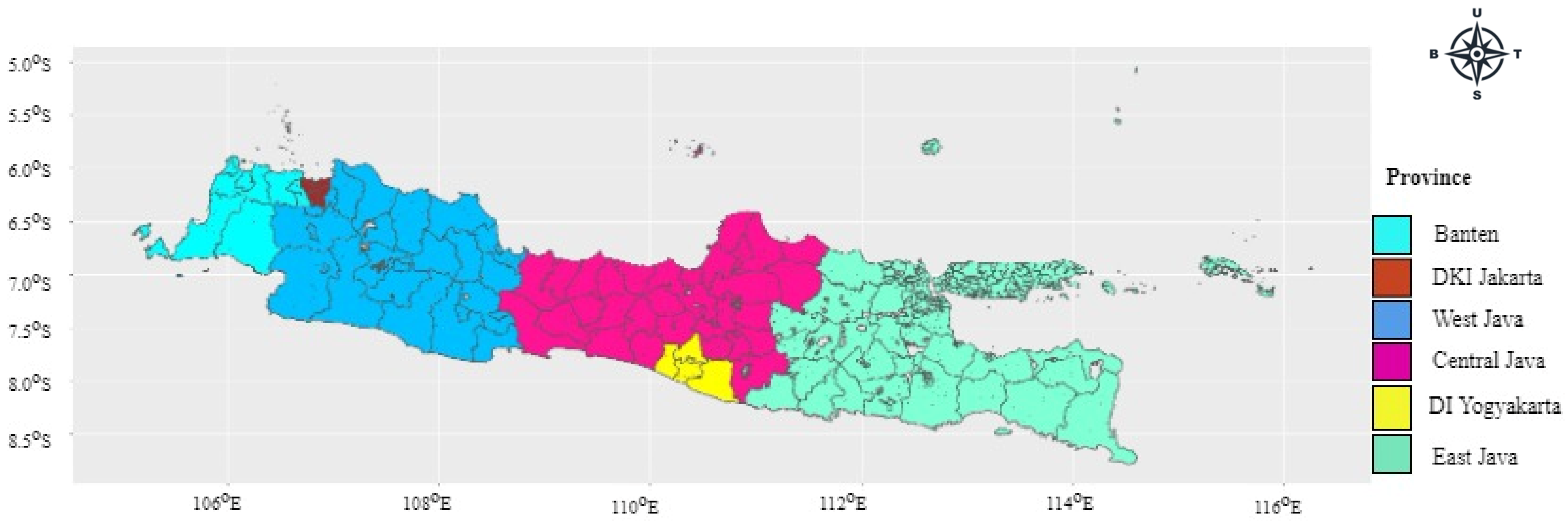
3.1. Research Location

In this study, we chose Java Island as one of the biggest islands in Indonesia. Administratively, as seen in Figure 2, Java Island has six provinces with 119 districts covering an area of about 128,297 square kilometers. In addition, Java is one of Indonesia’s most densely populated islands. It has a variety of terrain, including plains, mountains, and coastal regions. The choice of Java Island for this study is based on its heavy rainfall and frequent landslides and floods. The island is located near the equator, which has a tropical environment with heavy rains all year. On the other hand, Java Island has significant climatic diversity, with high variations in rainfall from one region to another. We implement our proposed technique, the SDM with Casetti expansion, to predict rainfall on Java Island so that we can make a better plan to reduce the risk of disasters caused by the rainfall problem.

3.2. Data Description

The objective of this study was to apply the Spatial Durbin Model (SDM) with expansion using Casetti’s approach to analyze climate data specific to Java Island, Indonesia. The study utilized secondary data sourced from the NASA POWER observation satellite, accessible through the data access viewer at https://power.larc.nasa.gov/data-access-viewer/, accessed on 5 July 2023). Notably, NASA POWER data are accessible under a General Public License, facilitating widespread usability. The dataset is extensive, comprising 6636.982 terabytes of recorded data (https://disc.gsfc.nasa.gov/, accessed 13 June 2024), encompassing domains such as agroclimatology, renewable energy, and sustainable buildings. Data availability spans various temporal resolutions, including hourly, daily, monthly, yearly, and climatology data in various formats including ASCII, CSV, GeoJSON, ICASA, and NetCDF.

The accessible parameters included solar fluxes and related temperatures/thermal iR flux, humidity/precipitation, wind/pressure, and soil properties. During the data collection phase, a rigorous parameter selection process was conducted to gather climatic variables specific to the Java Island region, encompassing six provinces and 119 districts/cities from January 1984 to July 2023, recorded on a monthly basis. The selected climate variables comprised rainfall, air temperature, humidity, solar irradiation, surface pressure, and geographical coordinates (latitude and longitude). The collected data were stored in comma-separated values (.csv) format.

This study focused specifically on precipitation parameters across Java Island’s 119 districts and cities using data accessed from the NASA POWER website, which provides Numerical Weather Prediction (NWP) data. Each coordinate point is represented by a grid resolution of (0.5 × 0.625)°, corresponding to approximately 50 km [34]. During data preprocessing, 55 duplicate locations were identified and removed, resulting in a dataset of 64 distinct districts/cities for subsequent predictive modeling, as detailed in

Table 1. Climate Variables Data of the 64 cities/districts of Java Island, Indonesia.

No.	Locations	Latitude	Longitude	Climate Variables (Averages)
				Rainfall (mm)	Air Temperature (°C)	Humidity (%)	Solar Irradiation (W/m2)	Surface Pressure (kPa)
1	Serang City	−6.15	106	166.53	27.08	81.47	17.63	100.51
2	Pandeglang	−6.3092	106.1047	173.91	25.49	84.50	17.63	98.27
3	Tangerang City	−6.171389	106.640556	175.80	27.20	81.44	17.63	100.81
4	South Tangerang City	−6.28577727	106.7122607	178.34	24.66	85.15	17.63	96.82
5	Kepulauan Seribu	−5.662900	106.568300	202.67	27.80	80.03	18.25	100.96
6	Central Jakarta	−6.170000	106.820000	175.80	27.20	81.44	17.63	100.81
7	Bekasi City	−6.241586	106.992416	175.80	27.20	81.44	17.63	100.81
8	Bogor City	−6.899541	107.533867	178.34	24.66	85.15	17.63	96.82
9	Indramayu	−6.327583	108.324936	184.87	26.40	80.98	18.75	99.66
10	Karawang	−6.32273	107.337579	190.09	25.25	83.46	18.28	97.86
…	…	…	…	…	…	…	…	…
64	Ponorogo	−7.8686	111.4619	163.89	24.98	82.55	19.48	97.43

. These distinct districts/cities can be further classified into six major provinces, namely, Banten, DKI Jakarta, Jawa Barat, Jawa Tengah, Daerah Istimewa Yogyakarta, and Jawa Timur. The comparison of climate variables across provinces in Indonesia reveals significant regional diversity in climate patterns. The average rainfall across the different cities/districts is 175.2 mm., with a range of 137.3 mm to 228.8 mm. However, rainfall shows considerable variation, with Jawa Barat and Jawa Tengah experiencing the widest range of levels, indicating distinct precipitation patterns across these provinces. Kota Tasikmalaya in the province of Jawa Barat has the highest reported rainfall and surface pressure. Surface pressure, ranging from 90.93 kPa to 100.96 kPa, with a mean of 97.90 kPa, remains generally stable with minor fluctuations observed among provinces. Humidity levels range from 75.46% to 89.10%, averaging 82.12%. Air temperature, varying between 21.36 °C and 27.90 °C, with an average of 25.50 °C, exhibits noticeable differences, with DKI Jakarta generally experiencing warmer conditions, while Jawa Barat tends to be cooler, and other provinces maintain moderate temperatures. Solar irradiation, which reflects sunlight exposure, shows notable variation across provinces in Indonesia. Banten exhibits lower levels of solar irradiation with a median of 17.63 W/m², while Jawa Timur displays higher levels with a median of 19.62 W/m². The remaining provinces demonstrate moderate to high exposure to sunlight. Among the cities/districts, Kab Situbondo of the province of Jawa Timur has the highest solar irradiation, but lowest rainfall level and surface pressure.

3.3. RShiny for SDM with Expansion Using Casetti’s Approach

The prediction procedure described in Section 2 was implemented through the development of an RShiny web application for the Spatial Durbin Model (SDM) with expansion using Casetti’s approach. This application is accessible via the following link: https://andriyanafalah.shinyapps.io/SDM-Expansion/ (accessed on 11 June 2024). The source code for the application is provided in Appendix B. The application features six dashboards, each serving a distinct purpose:

• Description of model: This section explains the formulation of the SDM with expansion using Casetti’s approach.
• Import data: In this section, users can upload data files in .csv or .txt format. The data should contain the coordinate of location (latitude and longitude), dependent variable and exogenous variables.
• Vector and matrix
  Construct vectors and matrices based on the data, as follows:
  • a.

    Vector $y$ defines the dependent variable at each location.

    b.

    Matrix $X$ and $\tilde{X}$ represent the exogenous variables.

    c.

    Matrix $Z$ consists of location coordinate entries in latitude and longitude.

    d.

    Matrix $J$ is an identity matrix with a size of as many as four exogenous variables according to the matrix $X$ or matrix $\tilde{X}$.

    e.

    Matrix $W$ is the result of calculating the inverse distance weight matrix using the equation with input location coordinates (latitude and longitude).

    f.

    Kronecker $Z$ is the expression obtained from the multiplication of the Kronecker with the identity matrix of exogenous variables $\left(Z\otimes I_k\right)$.

    g.

    Matrix $A$ is the product of matrix $X$, $Z$, and $J$.

    h.

    Matrix $\mathit{U}$ is the combination of vector 1, matrix $\mathbf{A}$, and the product of matrix $\mathbf{W}$ and $\tilde{\mathbf{X}}$.

• Result of prediction: This includes the calculation of results of parameter estimation $\widehat{\rho }$, $\widehat{\alpha }$, ${\widehat{\beta }}_0$, and $\widehat{\mathit{\theta }}$ obtaining the prediction results $\widehat{\mathit{y}}$, absolute error, and MAPE.
• Download data: This menu allows users to download the prediction calculation data.
• Created by: This section lists the names of the RShiny development team.

3.4. KDD for SDM with Expansion Using Casetti’s Approach

The research flowchart for the SDM with expansion using Casetti’s approach applied to climate data in Java Island, Indonesia, using the Knowledge Discovery in Databases (KDD) methodology, is depicted in Figure 3. Climate data from NASA POWER undergo a data preprocessing stage via an RShiny web application, accessible at https://annisanurfalah.shinyapps.io/Pre-ProcessingData/ (accessed on 26 September 2023). This stage includes variable selection, time transformation from daily to monthly data, and the removal of missing values and duplicates. As a result, climate variable data are obtained for 64 districts/cities as cross-sectional data. Furthermore, the pre-processed data are subsequently utilized as input for the data mining process. The results from the preprocessing stage are used to construct the inverse distance weight matrix, and spatial autocorrelation is assessed using Moran’s Index and Scatterplot. If spatial autocorrelation is detected, the process continues with the SDM with expansion using Casetti’s approach, employing the Maximum Likelihood Estimation (MLE) method. Parameter estimation for the SDM with expansion using Casetti’s approach is then calculated, followed by an evaluation of prediction accuracy using the Mean Absolute Percentage Error (MAPE). The prediction results are post-processed by visualizing spatial mapping through choropleth maps and providing interpretations to derive valuable insights.

3.5. Result of Moran’s Index and Scatterplot

The Moran Index was computed to assess the presence of spatial autocorrelation between the observation sites. Equation (4) was used to compute the Moran Index for each climate variable. The results of these calculations are presented in

Table 2. Spatial autocorrelation test for the climate variables.

No	Climate Variables	$\mathit{I}$	$\mathit{E}\left(\mathit{I}\right)$	$\mathit{V}\mathit{a}\mathit{r}\left(\mathit{I}\right)$	p-Value
1	$\mathit{y}$ (rainfall)	0.703	−0.016	0.004	$2.2\times {10}^{-16}$ *
2	${\mathit{X}}_1$ (air temperature)	0.376	−0.016	0.004	$2.084\times {10}^{-10}$ *
3	${\mathit{X}}_2$ (humidity)	0.527	−0.016	0.004	$2.2\times {10}^{-16}$ *
4	${\mathit{X}}_3$ (solar irradiation)	0.806	−0.015	0.005	$2.2\times {10}^{-16}$ *
5	${\mathit{X}}_4$ (surface pressure)	0.337	−0.016	0.004	$7.612\times {10}^{-9}$ *

* Significant at $\alpha =0.05$.

.

Based on Table 2, the p-values are all less than the significance level (5% even for 1%), indicating the presence of spatial autocorrelation. This suggests that the proximity between locations influences the climate variables. In addition to the Moran Index calculation, each region’s unique characteristics and the overall clustering tendency are shown using a Moran Scatterplot. For every unit of analysis, a four-quadrant graph serves as the visual representation. The mean and average lines delineate the four quadrants, which represent possible groupings. When an area’s numbers were higher than the average, it was seen to have high traits; when they were lower than the average, it was thought to have poor attributes. Figure 4 displays all of the Moran Scatterplot results for every climate variable.

Based on the results of the spatial autocorrelation test presented in Table 2 and the Moran Scatterplots depicted in Figure 4, a positive spatial autocorrelation is evident for all climate variables—rainfall, air temperature, humidity, solar irradiation, and surface pressure—across the 64 districts/cities of Java Island. Figure 4 clearly indicates this positive spatial autocorrelation, as shown by the increasing trends in quadrant I (high–high) and quadrant iII (low–low). This suggests that districts/cities with high values of climate variables are in spatial proximity to other districts and cities with similarly high values. Conversely, districts/cities with low values of climate variables tend to be situated near other districts/cities with low values of these variables.

3.6. Prediction Result of SDM with Expansion Using Casetti’s Approach

The estimation of prediction parameters in the SDM with expansion using Casetti’s Approach was conducted via the RShiny web application. An estimated $\widehat{\rho }$ value of 0.999 was obtained, producing an optimum spatial lag with a positive value $\left(\widehat{\rho }>0\right)$ and indicative of a spatial lag dependence. This $\widehat{\rho }$ value signifies the influence of adjacent locations within Java Island on rainfall prediction data. It further highlights the spatial autocorrelation of rainfall on Java Island, indicating that districts and cities with high rainfall levels tend to be spatially clustered with others exhibiting similar high rainfall levels, or with minimal variation. The results of the parameter estimate calculation ${\widehat{\mathit{\beta }}}_0$ and $\widehat{\mathit{\theta }}$ are shown in

Table 3. Parameter estimated value.

Coefficient	Parameter Estimated Value
		${\widehat{\mathit{\beta }}}_0$	$\widehat{\mathit{\theta }}$
${\mathit{X}}_1$ (air temperature)	${\widehat{\beta }}_{latitude}$	−7.994	11.969
	${\widehat{\beta }}_{longitude}$	17.524
${\mathit{X}}_2$ (humidity)	${\widehat{\beta }}_{latitude}$	2.312	−0.227
	${\widehat{\beta }}_{longitude}$	7.295
${\mathit{X}}_3$ (solar irradiation)	${\widehat{\beta }}_{latitude}$	−0.570	−6.869
	${\widehat{\beta }}_{longitude}$	−0.570
${\mathit{X}}_4$ (surface pressure)	${\widehat{\beta }}_{latitude}$	0.191	−8.393
	${\widehat{\beta }}_{longitude}$	0.456

.

The estimate ${\widehat{\mathit{\beta }}}_0$ measures the direct impact of the exogenous variables on rainfall levels within the same region, while the estimate $\widehat{\mathit{\theta }}$ captures the spillover effects of the exogenous variables on rainfall levels. Based on the estimate ${\widehat{\mathit{\beta }}}_0$, we can derive the estimate $\widehat{\mathit{\beta }}$, from which individual parameter estimates were derived for each exogenous variable across the 64 districts and cities. The SDM with expansion using Casetti’s approach produces different parameter estimates for each exogenous variable at each location due to the expansion of the exogenous variable matrix involving latitude and longitude information at each location. Detailed equations for the SDM with expansion using Casetti’s approach at each location are provided in Appendix A. A visualization of rainfall prediction in 64 districts/cities in Java Island is shown in Figure 5.

Based on Figure 5, the highest monthly rainfall predictions with values above 210 mm are in Pangandaran, Tasikmalaya City, Cilacap, Garut, Bandung and Bandung City. While the lowest monthly rainfall predictions with values below 140 mm are in Lumajang, Jember, Probolinggo, Probolinggo City, Situbondo, and Bondowoso. The proposed model has a MAPE value of 2.78%, indicating very accurate prediction. As observed from Section 3.2, these results are consistent with the rainfall patterns observed across cities/districts and provinces in Java Island.

4. Discussion

The Spatial Durbin Model (SDM) with expansion using Casetti’s approach was applied to analyze rainfall and climate variables across 64 districts/cities in Java Island, Indonesia, which is characterized by a monsoonal rainfall pattern. The prediction calculation employed an integrated R script developed for the SDM with expansion using Casetti’s approach, implemented through the RShiny web application, which comprises six interactive dashboards. The comprehensive source code is archived in a GitHub repository, with the link provided in Appendix B. This resource is instrumental for facilitating the replication and validation of both the model framework and findings by fellow researchers [35,36].

Moran’s Index and Scatterplots indicate that there is positive spatial autocorrelation among climate variables (rainfall, surface pressure, humidity, air temperature, and solar irradiation) across the 64 districts/cities of Java Island. This finding reveals that districts/cities with high values for climate variables tend to be spatially clustered with others exhibiting similarly high values, and vice versa. Previous research utilizing SAR-X with Casetti’s approach, as discussed by [16], did not account for spatial dependencies of exogenous variables, potentially leading to suboptimal results. To address this limitation, it is recommended to integrate these dependencies into the analysis through the Spatial Durbin Model (SDM). The model’s accuracy is supported by the precise estimation of parameter values assigned to each climate variable, contributing significantly to the high precision of the prediction results. Different parameter estimates were derived for each exogenous variable across the 64 districts/cities. This highlights that the SDM with expansion using Casetti’s approach generates distinct parameter estimates for each exogenous variable at each location. This is attributed to the expansion of the exogenous variable matrix involving latitude and longitude information at each location. The results showed the remarkable accuracy of the prediction outcomes obtained through the model at each observation location. The proposed SDM with expansion using Casetti’s approach resulted in a very accurate rainfall prediction with an MAPE of 2.78%. The summary of this study underscored that the level of rainfall in each region, based on the data from 64 districts/cities in Java Island, was significantly influenced by the other climate variable factors, such as air temperature, humidity, solar irradiation, and surface pressure [17].

5. Conclusions

In conclusion, this research underscored that the level of rainfall in each region, based on data from 64 districts/cities in Java Island, Indonesia, was significantly influenced by four other climate variable factors. Air temperature significantly impacts rainfall; the interactions are complex and can increase and decrease depending on the specific conditions and regions involved. Humidity is a critical factor in the formation and intensity of rainfall; the interplay between humidity and other atmospheric conditions determines the overall rainfall patterns in different regions. The effects of solar irradiation are integral to understanding diurnal and seasonal rainfall patterns and larger-scale climate phenomena such as monsoons. The interaction between high and low surface pressure systems and the resulting wind and moisture transport plays a critical role in determining rainfall patterns. It should be noted that these factors collectively exhibited a positive spatial autocorrelation across various areas. Climatological data most likely consist of extreme values. However, this can be addressed by developing a technique that uses a more robust objective function.

Accordingly, it is recommended that relevant institutions involved in rainfall prediction consider the multifaceted aspects of climate variables comprehensively. The modelling approach presented in this study facilitated a thorough understanding of how each climate variable influences specific locations. The findings from this study are anticipated to inform strategic decision-making at institutions such as BMKG and agribusiness companies, to enhance agricultural planning, optimize planting seasons, and disseminating crucial and valuable climate information to the general public, particularly regarding rainfall patterns.

6. Patents

Granted Copy Right: Copy Right for Computer Program, number 000624157.

Entitled “RShiny Web Application for Spatial Durbin Model with Expansion using Casetti’s Approach”, Ministry of Law and Human Rights of the Republic of Indonesia (Falah, A. N., Andriyana, Y.), 2024.

https://andriyanafalah.shinyapps.io/SDM-Expansion/ (accessed on 11 June 2024).

References

1. Gunawan, D. Peta Curah Hujan Ekstrem Indonesia Periode 1991–2020; BMKG: Jakarta, Indonesia, 2022. [Google Scholar]
2. Nurlatifah, A.; Hatmaja, R.B.; Rakhman, A.A. Analisis Potensi Kejadian Curah Hujan Ekstrem di Masa Mendatang Sebagai Dampak dari Perubahan Iklim di Pulau Jawa Berbasis Model Iklim Regional CCAM. J. Ilmu Lingkung. 2023, 21, 980–986. [Google Scholar] [CrossRef]
3. Kasa, A.N.G. Buletin Informasi Iklim November, No. 2. 2023; BMKG: Jakarta, Indonesia, 2023. [Google Scholar]
4. Kartika, Q.A.; Faqih, A.; Santikayasa, I.P.; Setiawan, A.M. Sea Surface Temperature Anomaly Characteristics Affecting Rainfall in Western Java, Indonesia. Agromet 2023, 37, 54–65. [Google Scholar] [CrossRef]
5. Aldrian, E.; Susanto, R.D. Identification of three dominant rainfall regions within Indonesia and their relationship to sea surface temperature. Int. J. Clim. 2003, 23, 1435–1452. [Google Scholar] [CrossRef]
6. Lee, H.S. General Rainfall Patterns in Indonesia and the Potential Impacts of Local Seas on Rainfall Intensity. Water 2015, 7, 1751–1768. [Google Scholar] [CrossRef]
7. Aldrian, E. Pemahaman Dinamika Iklim di Negara Kepulauan Indonesia Sebagai Modalitas Ketahanan Bangsa. J. Ilmu Pertan. Indones. 2016, 27, 606–613. [Google Scholar]
8. BMKG. Pemutakhiran Zona Musim Indonesia Periode 1991–2020; BMKG: Jakarta, Indonesia, 2022; p. 126. [Google Scholar]
9. SDGs Indonesia. Sustainable Development Goals (SDGs)-Tujuan 13; SDGs Indonesia: Jakarta, Indonesia, 2021. [Google Scholar]
10. Hatfield, G. Spatial statistics. In Practical Mathematics for Precision Farming; SSSA: Madison, WI, USA, 2018; pp. 75–104. [Google Scholar] [CrossRef]
11. Stohlgren, T.J. Spatial Analysis and Modeling. In Measuring Plant Diversity: Lessons from the Field; Oxford Academic: Oxford, UK, 2007; pp. 254–270. [Google Scholar] [CrossRef]
12. Triyatno, T.; Berd, I.; Idris. Spatial Model of Flood Hazard Due To Land Cover Change in the Tarusan Watershed, West Sumatra—Indonesia. Int. J. GEOMATE 2023, 25, 21–29. [Google Scholar] [CrossRef]
13. Bonsoms, J.; Ninyerola, M. Comparison of linear, generalized additive models and machine learning algorithms for spatial climate interpolation. Theor. Appl. Clim. 2024, 155, 1777–1792. [Google Scholar] [CrossRef]
14. Anna, A.N.; Fikriyah, V.N.; Ibrahim, M.H.; Ismail, K.; Pamekar, M.S.; Asshodiq, A.D.T. Spatial Modelling of Local Flooding for Hazard Mitigation in Surakarta, Indonesia. Int. J. GEOMATE 2021, 21, 145–152. [Google Scholar] [CrossRef]
15. Jalbert, J.; Genest, C.; Perreault, L. Interpolation of Precipitation Extremes on a Large Domain Toward IDF Curve Construction at Unmonitored Locations. J. Agric. Biol. Environ. Stat. 2022, 27, 461–486. [Google Scholar] [CrossRef]
16. Falah, A.N.; Ruchjana, B.N.; Abdullah, A.S.; Rejito, J. The Hybrid Modeling of Spatial Autoregressive Exogenous Using Casetti’ s Model Approach for the Prediction of Rainfall. Mathematics 2023, 11, 3783. [Google Scholar] [CrossRef]
17. Hermawan, E.; Lubis, S.W.; Harjana, T.; Purwaningsih, A.; Risyanto; Ridho, A.; Andarini, D.F.; Ratri, D.N.; Widyaningsih, R. Large-Scale Meteorological Drivers of the Extreme Precipitation Event and Devastating Floods of Early-February 2021 in Semarang, Central Java, Indonesia. Atmosphere 2022, 13, 1092. [Google Scholar] [CrossRef]
18. Anselin, L. Spatial Econometrics: Methods and Models. J. Am. Stat. Assoc. 1988, 85, 905. [Google Scholar]
19. LeSage, J. Spatial Econometrics Toolbox. In A Companion to Theoretical Econometrics; Blackwell: Oxford, UK, 1999; p. 273. [Google Scholar]
20. Lu, G.Y.; Wong, D.W. An adaptive inverse-distance weighting spatial interpolation technique. Comput. Geosci. 2008, 34, 1044–1055. [Google Scholar] [CrossRef]
21. Maria, E.; Budiman, E.; Haviluddin; Taruk, M. Measure distance locating nearest public facilities using Haversine and Euclidean Methods. J. Phys. Conf. Ser. 2020, 1450, 12080. [Google Scholar] [CrossRef]
22. Rosmanah, R.; Djara, V.A.D.; Andriyana, Y.; Jaya, I.G.N.M. The spatial econometrics of economic growth in Sumatera Utara province. J. Math. Comput. Sci. 2022, 12, 7283. [Google Scholar] [CrossRef]
23. Notonegoro, Y.; Andriyana, Y.; Ruchjana, B.N. Comparison of distance-based spatial weight matrix in modeling Internet signal strengths in Tasikmalaya regency using logistic spatial autoregressive model. Int. J. Data Netw. Sci. 2024, 8, 893–906. [Google Scholar] [CrossRef]
24. Kopczewska, K. Applied Spatial Statistics and Econometrics; Routledge: London, UK, 2020. [Google Scholar]
25. Lesage, J.; Pace, R.K. Introduction to Spatial Econometrics; CRC Press: Boca Raton, FL, USA, 2009. [Google Scholar]
26. Ord, K. Estimation Methods for Models of Spatial Interaction. J. Am. Stat. Assoc. 1975, 70, 120. [Google Scholar] [CrossRef]
27. Smirnov, O.; Anselin, L. Fast maximum likelihood estimation of very large spatial autoregressive models: A characteristic polynomial approach. Comput. Stat. Data Anal. 2001, 35, 301–319. [Google Scholar] [CrossRef]
28. Robinson, P.M.; Rossi, F. Refinements in maximum likelihood inference on spatial autocorrelation in panel data. J. Econ. 2015, 189, 447–456. [Google Scholar] [CrossRef]
29. Qiu, F.; Ding, H.; Hu, J. Asymptotic Properties of Quasi-Maximum Likelihood Estimators for Heterogeneous Spatial Autoregressive Models. Symmetry 2022, 14, 1894. [Google Scholar] [CrossRef]
30. Ezcurra, R.; Le Gallo, J.; Abate, G.D.; Chasco, C.; González-Val, R.; Elhorst, J.P. Theory and Practice of Spatial Econometrics. Spat. Econ. Anal. 2015, 10, 400. [Google Scholar] [CrossRef]
31. Lawrence, K.D.; Klimberg, R.K.; Lawrence, S.M. Fundamentals of Forecasting Using Excel; Industrial Press Inc.: New York, NY, USA, 2009. [Google Scholar]
32. Ishwarappa; Anuradha, J. A brief introduction on big data 5Vs characteristics and hadoop technology. Procedia Comput. Sci. 2015, 48, 319–324. [Google Scholar] [CrossRef]
33. Rohit, R.; Kapil, N.K.; Sandeep, K.; Ramya, L.K. Data Mining and Machine Learning Applications; Wiley-Scrivener: New York, NY, USA, 2022. [Google Scholar]
34. Qin, Y.; Zhang, P.; Liu, W.; Guo, Z.; Xue, S. The application of elevation corrected MERRA2 reanalysis ground surface temperature in a permafrost model on the Qinghai-Tibet Plateau. Cold Reg. Sci. Technol. 2020, 175, 103067. [Google Scholar] [CrossRef]
35. Zhang, C.; Hu, C.; Wu, T.; Zhu, L.; Liu, X. Achieving Efficient and Privacy-Preserving Neural Network Training and Prediction in Cloud Environments. IEEE Trans. Dependable Secur. Comput. 2022, 20, 4245–4257. [Google Scholar] [CrossRef]
36. Hu, C.; Zhang, C.; Lei, D.; Wu, T.; Liu, X.; Zhu, L. Achieving Privacy-Preserving and Verifiable Support Vector Machine Training in the Cloud. IEEE Trans. Inf. Forensics Secur. 2023, 18, 3476–3491. [Google Scholar] [CrossRef]
Figure 1. Rainfall Patterns in Indonesia. Source: Meteorology, Climatology, and Geophysics Agency (BMKG), Indonesia [8].
Mathematics 12 02304 g001
Figure 2. Research Location in Java Island, Indonesia.
Mathematics 12 02304 g002
Figure 3. KDD flowchart on the SDM with expansion using Casetti’s approach.
Mathematics 12 02304 g003
Figure 4. Moran’s Scatterplot of climate variables: (a) rainfall, (b) air temperature, (c) humidity, (d) solar irradiation, (e) surface pressure.
Mathematics 12 02304 g004
Figure 5. Visualization of rainfall prediction in 64 districts/cities in Java Island.
Mathematics 12 02304 g005