Maximizing Closeness in Bipartite Networks: A Graph-Theoretic Analysis

Abstract

A fundamental aspect of network analysis involves pinpointing nodes that hold significant positions within the network. Graph theory has emerged as a powerful mathematical tool for this purpose, and there exist numerous graph-theoretic parameters for analyzing the stability of the system. Within this framework, various graph-theoretic parameters contribute to network analysis. One such parameter used in network analysis is the so-called closeness, which serves as a structural measure to assess the efficiency of a node’s ability to interact with other nodes in the network. Mathematically, it measures the reciprocal of the sum of the shortest distances from a node to all other nodes in the network. A bipartite network is a particular type of network in which the nodes can be divided into two disjoint sets such that no two nodes within the same set are adjacent. This paper mainly studies the problem of determining the network that maximize the closeness within bipartite networks. To be more specific, we identify those networks that maximize the closeness over bipartite networks with a fixed number of nodes and one of the fixed parameters: connectivity, dissociation number, cut edges, and diameter.

1. Introduction

A network is typically depicted using an undirected simple graph, where nodes represent vertices and the connections between them are represented by edges. The central aspect of network analysis involves identifying which nodes hold significant positions within the network. Graph theory has become one of the most powerful mathematical tools in network analysis, offering numerous techniques and methodologies. One of the most important tasks of network analysis is to determine which nodes or links are more critical in a network. One such parameter, closeness, serves as a means of identifying nodes capable of efficiently disseminating information throughout the network. In simpler terms, a node with high closeness is one that can reach other nodes in the network quickly and efficiently. It signifies that the node is closely connected to the rest of the network and can potentially influence or be influenced by other nodes more rapidly than nodes with lower closeness values. Nodes with high closeness are crucial in various network applications, such as communication networks, social networks, and transportation networks, as they can facilitate rapid information flow, influence decision-making processes, and enhance overall network resilience. Thus, understanding the closeness of nodes provides valuable insights into the structural and functional characteristics of complex networks.

Closeness is measured on a scale from 0 to 1. A node with a value nearing 0 suggests it is relatively distant from other nodes within the network. Consequently, reaching other nodes from this point necessitates traversing numerous links. Conversely, a node with a value approaching 1 indicates it is in close proximity to other nodes. As a result, only a few connections are needed to reach neighbouring nodes from this node within the network.

Freeman first introduced the concept of closeness [1], but it turned out to be ineffective for disconnected graphs and exhibited weaknesses during graph operations. Addressing the first limitation, Latora and Marchiori introduced a novel measure of closeness for disconnected graphs [2], yet it still remains susceptible to the second weakness. Subsequently, Danglachev proposed an alternative definition [3], which effectively addresses the challenges posed by disconnected graphs and facilitates the creation of convenient formulas for graph operations. Following this definition of closeness, various vulnerability measures have been formulated to quantify the resilience of a network. Among these novel measures are the vertex (or edge) residual closeness parameters, which assess the closeness of a graph following the removal of vertices (or edges) [3]. Another measure is the additional closeness, which identifies the maximum potential of the closeness of a network, by means of the addition of a connection [4,5]. For further information on these new finer parameters, we recommend referring to [6,7,8,9,10,11,12].

The computation of closeness across various classes of graphs has gained significant attention in recent years [3,13,14,15]. For instance, Danglachev investigated the closeness of splitting graphs [16]. In [17], the same author determined the closeness of line graphs for certain fundamental graphs, as well as the closeness of line graphs connected by a bridge of two basic graphs. Closeness formulas for various graph classes were derived by Golpek [18]. Poklukar and Žerovnik [19] identified the graphs that minimize and maximize closeness among all connected graphs and trees with a fixed order, respectively. They also determined the graphs that uniquely maximize closeness among all cacti of fixed order and number of cycles, posing an open problem for the minimum case. The open problem posed by Poklukar and Žerovnik [19] was solved by Hayat and Xu [20], which obtained the unique graph that minimizes closeness across all cacti with fixed numbers of vertices and cycles. The notion of closeness in spectral graph theory was recently combined by Zheng and Zhou [21]. They also investigated the closeness matrix and established the connection between the closeness eigenvalues and the graph structure.

Basic Notations and Definitions

Let G be a simple connected graph with vertex set $V\left(G\right)$ and edge set $E\left(G\right)$. For a vertex $v\in V\left(G\right)$, $N_G\left(v\right)$ refers to the set of vertices adjacent to v in G. The degree of a vertex $v\in V\left(G\right)$, denoted by $d_G\left(v\right)$, is the number of vertices in $N_G\left(v\right)$. A pendent vertex in a graph is a vertex with degree one and an edge incident to a pendent vertex is called a pendent edge. For an edge $e\in E\left(G\right)$, $G-e$ denotes the subgraph of G obtained by removing e, and $G+xy$ represents a graph formed from G by adding an edge between x and y, where $x,y\in V\left(G\right)$. Deleting a vertex $v\in V\left(G\right)$ (along with its incident edges) from G is denoted by $G-v$. The union of two graphs $H_1$ and $H_2$, denoted by $H_1\cup H_2$ is the graph with $V(H_1\cup H_2)=V\left(H_1\right)\cup V\left(H_2\right)$ and $E(H_1\cup H_2)=E\left(H_1\right)\cup E\left(H_2\right)$. The join of two graphs $H_1$ and $H_2$, denoted by $H_1\vee H_2$ is a graph obtained from $H_1$ and $H_2$ by joining each vertex of $H_1$ to all vertices of $H_2$. For disjoint graphs $H_1,H_2,\dots ,H_t$ with $t\ge 3$, the sequential join $H_1\vee H_2\vee \cdots \vee H_t$ is the graph obtained from $H_1,H_2,\dots ,H_t$ by joining each vertex of $H_1$ to all vertices of $H_2$ and then joining each vertex of $H_2$ to all vertices of $H_3$, and continuing in this manner, finally connecting each vertex of $H_{t-1}$ to all vertices of $H_t$. For simplicity, $tG$ (and $\left[t\right]G$) is used to represent the union (and sequential join) of t disjoint copies of G. For example $t{K}_1=\overline{K_t}$ which is the t isolated vertices and $\left[a\right]H_1\vee H_2\vee \left[b\right]H_3$ is the sequential join $\underset{\mathrm{a}}{{\displaystyle \underbrace{H_1\vee H_1\vee \cdots \vee H_1}}}\vee H_2\vee \underset{\mathrm{b}}{{\displaystyle \underbrace{H_3\vee H_3\vee \cdots \vee H_3}}}$.

A matching in G is a set of edges that do not have a set of common vertices. A perfect matching in G is a matching that covers each vertex of G.

For vertices $u,v\in V\left(G\right)$, the distance between u and v in G is the length of the shortest path connecting them, and denoted by $d_G(u,v)$. Whereas, the diameter of G is the maximum distance between any pair of vertices in G.

By $P_n$ and $K_n$ we denote the path and complete graph on n vertices, respectively.

In [3], for a vertex u of G, the closeness of u in G is defined as

$$C_G\left(u\right)=\sum _{v\in V\left(G\right)\backslash \left\{u\right\}}{2}^{-d_G(u,v)}.$$

The closeness of G is defined as

$$C\left(G\right)=\sum _{u\in V\left(G\right)}{C}_G\left(u\right)=\sum _{u\in V\left(G\right)}\sum _{v\in V\left(G\right)\backslash \left\{u\right\}}{2}^{-d_G(u,v)}.$$

A bipartite graph is a graph in which $V\left(G\right)$ can be divided into two disjoint subsets $V_1$ and $V_2$ such that no two vertices within the same set are adjacent. A bipartite graph in which every two vertices from different partition classes are adjacent is called complete, and it is denoted by $K_{a,b}$, where $a=|V_1|,b=|V_2|$. Bipartite graphs serve as powerful tools for modeling complex systems with two distinct sets of entities, enabling analyses of and solutions to a wide range of real-world problems across different domains [22,23].

The (vertex) connectivity of a graph G is the minimum number of vertices whose removal from G results in a disconnected graph or in the trivial graph, and it is denoted by $k\left(G\right)$. If G is trivial or disconnected, then $k\left(G\right)=0$, obviously. An edge e of a connected graph G is a cut edge if $G-e$ is disconnected. A subset $M\subseteq V\left(G\right)$ is called a dissociation set if the induced subgraph $G\left[M\right]$ does not include $P_3$ as a subgraph. A maximum dissociation set of G is one with the greatest cardinality. Finally, the dissociation number of G is the cardinality of a maximum dissociation set within G.

In order to explore the connection between closeness and the structural characteristics of a graph, we will investigate extremal problems aimed at maximizing closeness within certain classes of bipartite graphs.

2. Main Results

In this section we will state our results. Specifically, we will determine those graphs which maximize closeness over the bipartite graphs of order n and one of the fixed parameters, such as dissociation number, connectivity, cut edges, and diameter.

The following Lemma will be helpful for the proofs of the main results.

Lemma 1 

([3,12]). If u and v are vertices in a graph G where there is no edge between them, then adding the edge $uv$ increases the closeness of G.

Our first main result establishes an upper bound on the closeness of a bipartite graphs with a fixed order and dissociation number $\alpha$, and identified the graph that attain the bound.

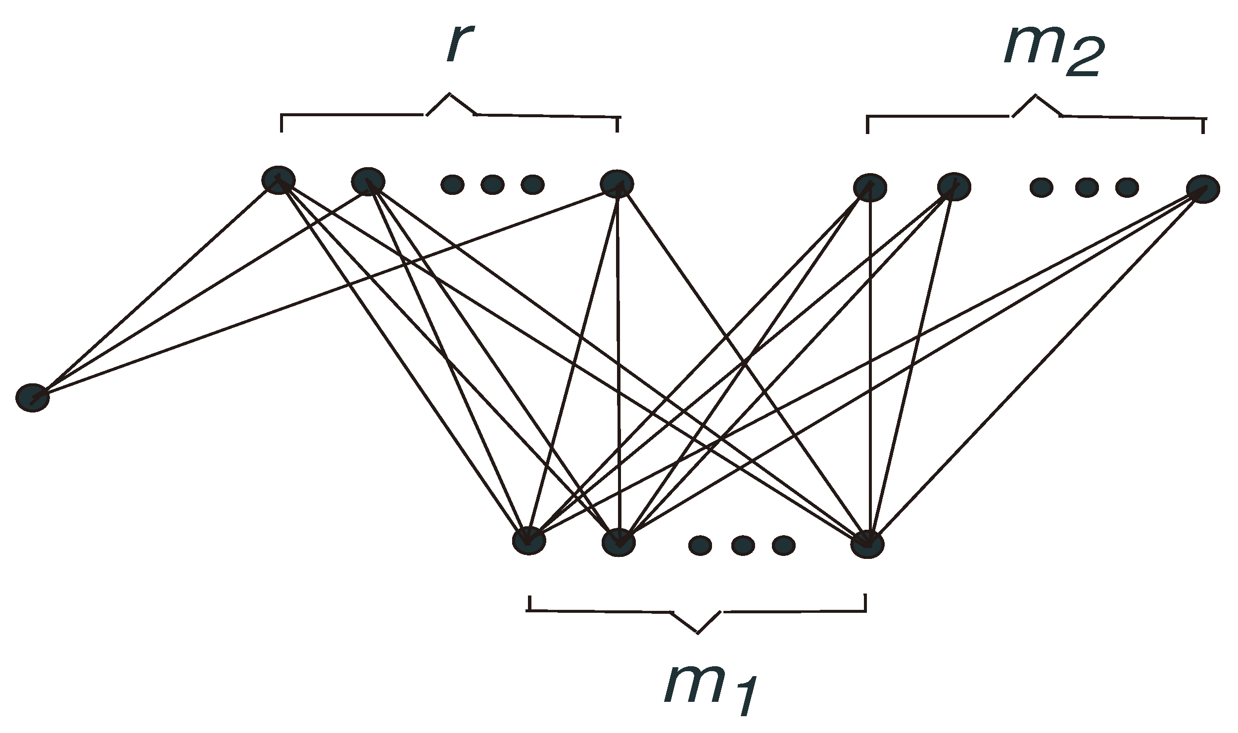
Theorem 1. 

Let G be a bipartite graph of order n with dissociation number α. Then,

$$C\left(G\right)\le \frac{n(n-1)}{4}+\frac{\alpha (n-\alpha )}{2}$$

with equality if and only if $G\cong K_{\alpha ,n-\alpha }$.

For $r\ge 1$, we define $N_r$ as the graph comprising r isolated vertices. Let $B_r(m_1,m_2)$ be the graph obtained from $N_r$ and $K_1\cup K_{m_1,m_2}$ by adding the edges between the vertices in $N_r$ and the vertices belonging to partitions of size $m_1$ in $K_{m_1,m_2}$ and $K_1$, respectively (see Figure 1). It is evident that $K_{r,n-r}=B_r(n-r-1,0)$.

Figure 1. The graph $B_r(m_1,m_2)$.

Our second result identifies the graph that maximizes the closeness within bipartite graphs of order n and fixed connectivity r.

Theorem 2. 

Let G be a bipartite graph of order n with connectivity r, where $1\le r\le \lfloor \frac{n-1}{2}\rfloor$. Then,

$$\begin{array}{ccc}\hfill C\left(G\right)& \le & \frac{1}{4}\left(⌈\frac{n-2r-1}{2}⌉+6r+1\right)⌈\frac{n-2r-1}{2}⌉+⌈\frac{n-2r-1}{2}⌉⌊\frac{n-2r-1}{2}⌋\hfill \\ & +& \frac{1}{4}\left(⌊\frac{n-2r-1}{2}⌋+6r\right)⌊\frac{n-2r-1}{2}⌋+\frac{r(3r+2)}{2}\hfill \end{array}$$

with equality if and only if $G\cong B_r\left(⌈\frac{n-2r-1}{2}⌉+r,⌊\frac{n-2r-1}{2}⌋\right)$.

For positive integers s, ℓ, and n, where $2\le s\le \frac{n-\ell }{2}$, let $A_{\ell }(s,n-s-\ell )$ be the graph obtained by attaching ℓ pendent vertices to a vertex with degree $n-s-\ell$ in $K_{s,n-s-\ell }$ (see Figure 2).

Figure 2. The graph $A_{\ell }(s,n-s-\ell )$.

The next result characterizes all bipartite graphs with n vertices and ℓ cut edges having the largest closeness.

Theorem 3. 

Let G be a bipartite graph of order $n\ge 5$ with ℓ cut edges.

(i) 

If $\ell =n-1$, then $C\left(G\right)\le \frac{(n-1)(n+2)}{4}$ with equality if and only if $G\cong K_{1,n-1}$;

(ii) 

If $\frac{3n}{4}-3\le \ell \le n-4$, then $C\left(G\right)\le \frac{n^2+3n-3\ell -8}{4}$ with equality if and only if $G\cong A_{\ell }(2,n-2-\ell )$.

In the following cases, $1\le \ell \le \frac{3n}{4}-3$.

(iii) 

If $3n-4\ell \equiv 0($mod $6)$, then $C\left(G\right)\le \frac{27n^2-18n+20{\ell }^2+54\ell -27n\ell }{72}$ with equality if and only if $G\cong A_{\ell }(\frac{n}{2}-\frac{2\ell }{3},\frac{n}{2}-\frac{\ell }{3})$;

(iv) 

If $3n-4\ell \equiv 1($mod $6)$, then $C\left(G\right)\le \frac{27n^2-18n+20{\ell }^2+55\ell -27n\ell -1}{72}$ with equality if and only if $G\cong A_{\ell }(\frac{n}{2}-\frac{2\ell }{3}-\frac{1}{6},\frac{n}{2}-\frac{\ell }{3}+\frac{1}{6})$;

(v) 

If $3n-4\ell \equiv 2($mod $6)$, then $C\left(G\right)\le \frac{27n^2-18n+20{\ell }^2+56\ell -27n\ell -4}{72}$ with equality if and only if $G\cong A_{\ell }(\frac{n}{2}-\frac{2\ell }{3}-\frac{1}{3},\frac{n}{2}-\frac{\ell }{3}+\frac{1}{3})$;

(vi) 

If $3n-4\ell \equiv 3($mod $6)$, then $C\left(G\right)\le \frac{27n^2-18n+20{\ell }^2+57\ell -27n\ell -9}{72}$ with equality if and only if $G\cong A_{\ell }(\frac{n}{2}-\frac{2\ell }{3}-\frac{1}{2},\frac{n}{2}-\frac{\ell }{3}+\frac{1}{2})$;

(vii) 

If $3n-4\ell \equiv 4($mod $6)$, then $C\left(G\right)\le \frac{27n^2-18n+20{\ell }^2+52\ell -27n\ell -4}{72}$ with equality if and only if $G\cong A_{\ell }(\frac{n}{2}-\frac{2\ell }{3}+\frac{1}{3},\frac{n}{2}-\frac{\ell }{3}-\frac{1}{3})$;

(viii) 

If $3n-4\ell \equiv 5($mod $6)$, then $C\left(G\right)\le \frac{27n^2-18n+20{\ell }^2+53\ell -27n\ell -1}{72}$ with equality if and only if $G\cong A_{\ell }(\frac{n}{2}-\frac{2\ell }{3}+\frac{1}{6},\frac{n}{2}-\frac{\ell }{3}-\frac{1}{6})$.

In a bipartite graph G with n vertices and diameter d, suppose $P=u_0{u}_1\cdots u_d$ represents a diametrical path of G. We can then partition $V\left(G\right)$ as follows:

$$V\left(G\right)=X_0\cup X_1\cup \cdots \cup X_d,$$

(1)

where $X_0=u_0$ and $X_i=v\in V\left(G\right):d_G(v,u_0)=i$ for $i=1,2,\dots ,d$.

Let

$$F(n,d)=[(d-1)/2]K_1\vee \lfloor (n-d-1)/2\rfloor K_1\vee \lceil (n-d-1)/2\rceil K_1\vee [(d-1)/2]K_1,$$

where d is odd. Let

$$\mathcal{H}(n,d)=\{H(n,d)=[d/2-1]K_1\vee a{K}_1\vee \lfloor (n-d+2)/2\rfloor K_1\vee b{K}_1\vee [d/2-1]K_1\},$$

where d is even, and $a+b=\lceil (n-d+2)/2\rceil$.

Clearly, $F(n,d)$ is a bipartite graph of order n with diameter d, and $\mathcal{H}(n,d)$ is a set of n-vertex bipartite graphs having diameter d.

Evidently, $K_2$ (resp. $P_n$) is the unique bipartite graph of diameter one (resp. $n-1$). In what follows, we consider $2\le d\le n-2$.

Our last main result identifies the bipartite graphs with n vertices and diameter d that maximize the closeness.

Theorem 4. 

Let G be a bipartite graph of order n with diameter d having maximum closeness.

$\left(i\right)$ If $d=2$, then $G\cong K_{\lfloor \frac{n}{2}\rfloor ,\lceil \frac{n}{2}\rceil }$;

$\left(ii\right)$ If $d\ge 3$, then $G\cong F(n,d)$ for odd d, and $G\in \mathcal{H}(n,d)$ otherwise.

3. Proof of Theorem 1

In this section, we give the proof of Theorem 1, which establishes an upper bound on the closeness of a bipartite graphs with a fixed order and dissociation number $\alpha$, and we identify the graph that attains the bound.

Proof. 

Let G be a bipartite graph of order n and dissociation number $\alpha$ that maximizes $C\left(G\right)$. Denote the partition of $V\left(G\right)$ as $(V_1,V_2)$, assuming without loss of generality that $|V_1|\ge |V_2|$. Let Q be the maximum dissociation set of G. Then $|V_1|\le |Q|=\alpha$. If $|V_1|=\alpha$, then by Lemma 1, $G\cong K_{\alpha ,n-\alpha }$.

Now, we consider the case where $|V_1|<\alpha$. Let $Q=Q_1\cup Q_2$ with $Q_1\subseteq V_1$, $Q_2\subseteq V_2$, and $Q_1^{\prime }=Q\backslash Q_1$, $Q_2^{\prime }=Q\backslash Q_2$. It can be observed that $|Q_2^{\prime }|<|Q_1|$ and $|Q_1^{\prime }|<|Q_2|$. Since G is a bipartite graph with maximum closeness, by Lemma 1, each vertex in $Q_1$ (resp. $Q_1^{\prime }$) is adjacent to each vertex in $Q_2$ (resp. $V_2$).

If $|Q_1|\le |Q_2|$, then there exists $S\subseteq Q_2$ with $|Q_2|=|S|$ such that $G[Q_1\cup S]$ forms a perfect matching. Thus, we have:

$$\begin{array}{cc}\hfill C\left(G\right)=& \frac{1}{4}\left[2|Q_1||Q_1^{\prime }|+2|Q_2^{\prime }||Q_2|+|Q_1|(|Q_1|-1)+|Q_2|(|Q_2|-1)+|Q_1^{\prime }|(|Q_1^{\prime }|-1)\right.\hfill \\ \hfill & \left.+|Q_2^{\prime }|(|Q_2^{\prime }|-1)\right]+\frac{1}{2}\left[2|Q_1||Q_1^{\prime }|+2|Q_1^{\prime }||Q_2^{\prime }|+2|Q_1^{\prime }||Q_2|+2|Q_1|\right]\hfill \\ \hfill & +\frac{1}{8}\left[2|Q_1|(|Q_1|-1)+2|Q_1|(|Q_2|-|Q_1|)\right],\hfill \end{array}$$

and

$$\begin{array}{cc}\hfill C\left(K_{|Q_1|+|Q_2|,|Q_1^{\prime }|+|Q_2^{\prime }|}\right)=& \frac{1}{4}\left[(|Q_1|+|Q_2|)(|Q_1|+|Q_2|-1)+(|Q_1^{\prime }|+|Q_2^{\prime }|)(|Q_1^{\prime }|+|Q_2^{\prime }|-1)\right]\hfill \\ \hfill & +\frac{1}{2}\left[2(|Q_1|+|Q_2|)(|Q_1^{\prime }|+|Q_2^{\prime }|)\right].\hfill \end{array}$$

We deduce,

$$\begin{array}{cc}\hfill C\left(G\right)-C\left(K_{|Q_1|+|Q_2|,|Q_1^{\prime }|+|Q_2^{\prime }|}\right)=& \frac{1}{4}\left[|Q_1|(3+2|Q_1^{\prime }|-4|Q_2^{\prime }|-|Q_2|)\right]+\frac{1}{2}\left[|Q_2^{\prime }|(|Q_1^{\prime }|-|Q_2|)\right].\hfill \end{array}$$

Note that since G is connected, we have $max|Q_1^{\prime }|,|Q_2^{\prime }|\ge 1$. If $|Q_1^{\prime }|=0$, then $|Q_2^{\prime }|\ge 1$, implying $2\le |Q_1|\le |Q_2|$. If $|Q^{\prime }1|\ge 1$, then $2\le |Q_2|$, and thus $C\left(G\right)<C(K|Q_1|+|Q_2|,$

$|Q_1^{\prime }|+|Q^{\prime }2|)$, which contradicts $\alpha \left(G\right)=|Q|=|Q_1|+|Q_2|=\alpha \left(K|Q_1|+|Q_2|,|Q_1^{\prime }|+|Q_2^{\prime }|\right)$.

If $|Q_1|>|Q_2|$, then by a similar argument as above, we arrive at a contradiction to the choice of G. Therefore, $G\cong K_{\alpha ,n-\alpha }$. By direct calculation, we obtain:

$$\begin{array}{ccc}\hfill C\left(K_{\alpha ,n-\alpha }\right)& =& \left[\alpha (\alpha -1)+(n-\alpha )(n-\alpha -1)\right]\times 2^{-2}+\left[2\alpha (n-\alpha )\right]\times 2^{-1}\hfill \\ & =& \frac{n(n-1)}{4}+\frac{\alpha (n-\alpha )}{2}.\hfill \end{array}$$

□

4. Proof of Theorem 2

To establish the main result, we first require the following Lemma.

Lemma 2. 

Let $a,b$ and r be positive integers.

$\left(i\right)$ If $r+b>a$, then $C\left(B_r(a,b)\right)<C\left(B_r(a+1,b-1)\right)$;

$\left(ii\right)$ If $r+b+1<a$, then $C\left(B_r(a,b)\right)<C\left(B_r(a-1,b+1)\right)$.

Proof. 

By the definition of closeness, we have

$$\begin{array}{cc}\hfill C\left(B_r(a,b)\right)=& [2a+2rb+r(r-1)+a(a-1)+b(b-1)]\times 2^{-2}\hfill \\ \hfill & +(2r+2ra+2ab)\times 2^{-1}+2b\times 2^{-3},\hfill \end{array}$$

$$\begin{array}{cc}\hfill C\left(B_r(a+1,b-1)\right)=& [2(a+1)+2r(b-1)+r(r-1)+a(a+1)+(b-1)(b-2)]\times 2^{-2}\hfill \\ \hfill & +[2r+2r(a+1)+2(a+1)(b-1)]\times 2^{-1}+2(b-1)\times 2^{-3},\hfill \end{array}$$

and

$$\begin{array}{cc}\hfill C\left(B_r(a-1,b+1)\right)=& [2(a-1)+2r(b+1)+r(r-1)+(a-1)(a-2)+b(b+1)]\times 2^{-2}\hfill \\ \hfill & +[2r+2r(a-1)+2(a-1)(b+1)]\times 2^{-1}+2(b+1)\times 2^{-3}.\hfill \end{array}$$

$\left(i\right)$ If $r+b>a$, we have

$$\begin{array}{cc}\hfill & C\left(B_r(a,b)\right)-C\left(B_r(a+1,b-1)\right)\hfill \\ \hfill & =(2r-2a+2b-4)\times 2^{-2}+(-2r+2a-2b+2)\times 2^{-1}+2\times 2^{-3}\hfill \\ \hfill & =[2a+1-2(b+r)]\times 2^{-2}<0.\hfill \end{array}$$

Thus, $C\left(B_r(a,b)\right)<C\left(B_r(a+1,b-1)\right).$

$\left(i\right)$ If $r+b+1<a$, we have

$$\begin{array}{cc}\hfill & C\left(B_r(a,b)\right)-C\left(B_r(a-1,b+1)\right)\hfill \\ \hfill & =(-2r+2a-2b)\times 2^{-2}+(2r-2a+2b+2)\times 2^{-1}-2\times 2^{-3}\hfill \\ \hfill & =[-2a+2(b+r+1)+1]\times 2^{-2}<0.\hfill \end{array}$$

Thus, $C\left(B_r(a,b)\right)<C\left(B_r(a-1,b+1)\right).$ □

By Lemma 3 $\left(ii\right)$, we immediately get the following Corollary.

Corollary 1. 

If $1\le r\le \lfloor \frac{n-1}{2}\rfloor$, then $C\left(K_{r,n-r}\right)<C\left(B_r(n-r-2,1)\right)$.

Proof. 

By direct calculation, we have

$$\begin{array}{cc}\hfill & C\left(B_r\left(⌈\frac{n-2r-1}{2}⌉+r,⌊\frac{n-2r-1}{2}⌋\right)\right)\hfill \\ \hfill =& \frac{1}{2}\left[2r+2r\left(⌈\frac{n-2r-1}{2}⌉+r\right)+2\left(⌈\frac{n-2r-1}{2}⌉+r\right)⌊\frac{n-2r-1}{2}⌋\right]\hfill \\ \hfill & +\frac{1}{4}\left[2\left(⌈\frac{n-2r-1}{2}⌉+r\right)+\left(⌈\frac{n-2r-1}{2}⌉+r\right)\left(⌈\frac{n-2r-1}{2}⌉+r-1\right)\right.\hfill \\ \hfill & +\left.⌊\frac{n-2r-1}{2}⌋\left(⌊\frac{n-2r-1}{2}⌋-1\right)+2r⌊\frac{n-2r-1}{2}⌋+r(r-1)\right]+\frac{2}{8}⌊\frac{n-2r-1}{2}⌋\hfill \\ \hfill =& \frac{1}{4}\left(⌈\frac{n-2r-1}{2}⌉+6r+1\right)⌈\frac{n-2r-1}{2}⌉+⌈\frac{n-2r-1}{2}⌉⌊\frac{n-2r-1}{2}⌋\hfill \\ \hfill & +\frac{1}{4}\left(⌊\frac{n-2r-1}{2}⌋+6r\right)⌊\frac{n-2r-1}{2}⌋+\frac{r(3r+2)}{2}.\hfill \end{array}$$

Let G be a bipartite graph of order n and connectivity r such that $C\left(G\right)$ is maximized. Let $W\subseteq G$ contain r vertices, and let $H_1,H_2,\dots ,H_k$ be the components of $G-W$, where $k\ge 2$. If any component $H_i$ of $G-W$ contains at least two vertices, then by Lemma 1, it must be a complete bipartite graph. If one of the components is a singleton set, denoted as $H_i=v$, then v is adjacent to all vertices in W; otherwise, if G’s connectivity is less than r, $G\left[W\right]$ contains isolated vertices.

Case 1. 

At least one component of $G-W$ comprises a minimum of two vertices.

In this case, $G-W$ comprises exactly two components. Otherwise, by introducing some edges in G, we would obtain a complete bipartite graph $G^{\prime }$ among the vertices of $H_1\cup H_2\cup \cdots \cup H_{k-1}$, with order n and connectivity r. According to Lemma 1, $C\left(G\right)<C\left(G^{\prime }\right)$, contradicting the maximality of G. Let $H_1$ and $H_2$ be the components of G. Then either $H_1=K_1$ or $H_2=K_1$. Otherwise, $G-U$ has the partitions $(M_1,M_2)$ and $(Q_1,Q_2)$, respectively. Let $W=W_1\cup W_2$ represent the bipartition of W. As G possesses maximum closeness, by Lemma 1, there must exist edges between the vertices of $M_1$ and $M_2$, $Q_1$ and $Q_2$, $W_1$ and $W_2$. Considering the definition of closeness, we have:

$$\begin{array}{cc}\hfill C\left(G\right)=& \frac{1}{4}\left[2|M_1||W_1|+2|M_1||Q_1|+2|M_2||Q_2|+2|M_2||W_2|+2|W_1||Q_1|+2|W_2||Q_2|\right.\hfill \\ \hfill & +|M_1|(|M_1|-1)+|M_2|(|M_2|-1)+|Q_1|(|Q_1|-1)+|Q_2|(|Q_2|-1)\hfill \\ \hfill & \left.+|W_1|(|W_1|-1)+|W_2|(|W_2|-1)\right]+\frac{1}{8}\left[2|M_1||Q_2|+2|M_2||Q_1|\right]\hfill \\ \hfill & +\frac{1}{2}\left[2|M_1|(|M_2|+|W_2|)+2|W_1|(|M_2|+|W_2|+|Q_2|)+2|Q_1|(|W_2|+|Q_2|)\right].\hfill \end{array}$$

Note that $|W_2|+|Q_2|\ge |W|$, and $|Q_2|\ge |W_1|$. Let $Q_2=YUZ$, and $G^{\prime }=G-\{q_{1}z:q_1\in V\left(Q_1\right),z\in V\left(Z\right)\}+\{m_1{q}_2:m_1\in V\left(M_1\right),q_2\in V\left(Q_2\right)\}+\{q{m}_2:q\in V\left(Q_1\right)\backslash \left\{q_1\right\},m_2\in V\left(M_2\right)\}$. Clearly, $G^{\prime }$ is a bipartite graph of order n having vertex cut $W_2\cup Y$ contain r vertices. We have

$$\begin{array}{cc}\hfill C\left(G^{\prime }\right)=& \frac{1}{4}\left[\right(|M_1|+|Q_1|+|W_1|)(|M_1|+|Q_1|+|W_1|-1)\hfill \\ \hfill & +(|M_2|+|Q_2|+|W_2|)(|M_2|+|Q_2|+|W_2|-1)]+\frac{1}{8}[2|M_2|+2|Q_2|-2|W_1|]\hfill \\ \hfill & +\frac{1}{2}\left[2(|M_1|+|Q_1|+|W_1|-1)(|M_2|+|Q_2|+|W_2|)+2(|W_1|+|W_2|)\right].\hfill \end{array}$$

So

$$\begin{array}{cc}\hfill C\left(G\right)-C\left(G^{\prime }\right)=& -\frac{3}{4}\left[|M_2|(|Q_1|-1)+|Q_2|(|M_1|-1)+|W_1|\right]<0\hfill \end{array}$$

this leads to a contradiction. Without loss of generality, let us assume that $H_2=K_1=u$. Then, $H_1=K_{a,b}$, and u is connected to all vertices of W, while each vertex of W is connected to every vertex of $H_1$ that is in the same partition as u. Thus, $G=B_r(a,b)$, where $r=|W|$, and $a\ge r$. Since G maximizes closeness, by Lemma 3, we have $r+b-1\le a\le r+b+1$, which implies $G\cong B_r\left(⌈\frac{n-2r-1}{2}⌉+r,⌊\frac{n-2r-1}{2}⌋\right)$.

Case 2. 

All components of $G-W$ consist of a single vertex.

In this case $G=K_{n-r,r}$. By Corollary 1, $k\ge \lfloor \frac{n-1}{2}\rfloor$.

Hence, $G\cong B_r\left(⌈\frac{n-2r-1}{2}⌉+r,⌊\frac{n-2r-1}{2}⌋\right)$. □

5. Proof of Theorem 3

Lemma 3 

([19]). Let G represent a connected graph containing a cut edge $e=uv$. Let $G^{\prime }$ denote the graph resulting from contracting edge e into a new vertex w, which becomes adjacent to every vertex in $N_G\left(u\right)\cup N_G\left(v\right)$ except for u and v, and then attaching a pendent edge at w. Then $C\left(G^{\prime }\right)>C\left(G\right)$.

Lemma 4. 

Let $u,v$ be the two vertices on the same partition of a complete bipartite graph H, and G be a graph formed from H by attaching pendent vertices $x_1,x_2,\dots ,x_s$ (resp. $y_1,y_2,\dots ,y_t$) to u (resp. v) . Let $G^{\prime }=G-\{u{x}_i:i=1,2,\dots ,s\}+\{v{x}_i:i=1,2,\dots ,s\}$. Then, $C\left(G^{\prime }\right)>C\left(G\right)$.

Proof. 

By the definition of closeness, we have

$$\begin{array}{ccc}& & C\left(G^{\prime }\right)-C\left(G\right)\hfill \\ & =& 2\sum _{i=1}^s\left(2^{-d_{G^{\prime }}(x_i,u)}-2^{-d_G(x_i,u)}\right)+2\sum _{i=1}^s\left(2^{-d_{G^{\prime }}(x_i,v)}-2^{-d_G(x_i,v)}\right)\hfill \\ & +& 2\sum _{i=1}^s\sum _{j=1}^t\left(2^{-d_{G^{\prime }}(x_i,y_j)}-2^{-d_G(x_i,y_j)}\right)\hfill \\ & =& 2\sum _{i=1}^s\left(2^{-[d_G(x_i,u)+2]}-2^{-d_G(x_i,u)}\right)+2\sum _{i=1}^s\left(2^{-[d_G(x_i,v)-2]}-2^{-d_G(x_i,v)}\right)\hfill \\ & +& 2\sum _{i=1}^s\sum _{j=1}^t\left(2^{-[d_G(x_i,y_j)-2]}-2^{-d_G(x_i,y_j)}\right)\hfill \\ & =& 2\sum _{i=1}^s{2}^{-d_G(x_i,u)}[2^{-2}-1]+2\sum _{i=1}^s{2}^{-d_G(x_i,u)}[2^{-2}-1]\hfill \\ & +& 2\sum _{i=1}^s\sum _{j=1}^t{2}^{-d_G(x_i,y_j)}[2^{-2}-1]\hfill \\ & =& \frac{6a+3ab}{8}>0.\hfill \end{array}$$

Hence, $C\left(G^{\prime }\right)>C\left(G\right)$. □

Lemma 5. 

Let $K_{p,q}$ be a graph with vertex partition $V_p=\{x_1,\dots ,x_p\}$ and $V_q=\{y_1,\dots ,y_q\}$, and G be a graph obtained from $K_{p,q}$ by attaching pendent vertices $a_1,a_2,\dots ,a_s$ (resp. $b_1,b_2,\dots ,b_t$) to $x_2$ (resp. $y_2$) . Let $G^{\prime }=G-\{x_2{a}_i:i=1,2,\dots ,s\}+\{y_2{a}_i:i=1,2,\dots ,s\}$. Then, $C\left(G^{\prime }\right)>C\left(G\right)$.

Proof. 

By the definition of closeness, we have

$$\begin{array}{ccc}& & C\left(G^{\prime }\right)-C\left(G\right)\hfill \\ & =& 2\sum _{i=1}^s\sum _{j=1}^t\left(2^{-d_{G^{\prime }}(a_i,b_j)}-2^{-d_G(a_i,b_j)}\right)+2\sum _{i=1}^s\sum _{j=1}^p\left(2^{-d_{G^{\prime }}(a_i,x_j)}-2^{-d_G(a_i,x_j)}\right)\hfill \\ & +& 2\sum _{i=1}^s\sum _{j=1}^q\left(2^{-d_{G^{\prime }}(a_i,y_j)}-2^{-d_G(a_i,y_j)}\right)\hfill \\ & =& 2\sum _{i=1}^s\sum _{j=1}^t\left(2^{-[d_G(a_i,b_j)-1]}-2^{-d_G(a_i,b_j)}\right)+2\sum _{i=1}^s\sum _{j=1}^p\left(2^{-[d_G(a_i,x_j)+1]}-2^{-d_G(a_i,x_j)}\right)\hfill \\ & +& 2\sum _{i=1}^s\sum _{j=1}^q\left(2^{-[d_G(a_i,y_j)-1]}-2^{-d_G(a_i,y_j)}\right)\hfill \\ & =& 2\sum _{i=1}^s\sum _{j=1}^t{2}^{-d_G(a_i,b_j)}[2-1]+2\sum _{i=1}^s\sum _{j=1}^p{2}^{-d_G(a_i,x_j)}[2^{-1}-1]\hfill \\ & +& 2\sum _{i=1}^s\sum _{j=1}^q{2}^{-d_G(a_i,y_j)}[2-1]\hfill \\ & =& \frac{ab}{4}>0.\hfill \end{array}$$

Hence, $C\left(G^{\prime }\right)>C\left(G\right)$. □

Proof. 

For $\ell =n-1$, $K_{1,n-1}$ stands as the unique bipartite graph, with its closeness calculated directly as $C\left(K_{1,n-1}\right)=\frac{(n-1)(n+2)}{4}$.

Consider a bipartite graph G of order n containing ℓ cut edges, maximizing $C\left(G\right)$. Note that for any bipartite graph with ℓ cut edges, $\ell \ne n-2$ and $\ell \ne n-3$. Hereafter, we consider the case $1\le \ell \le n-4$. Let $e_1,e_2,\dots ,e_{\ell }$ denote the ℓ cut edges of G. Our claim is that each component of $G\backslash \left\{e_1,e_2,\dots ,e_{\ell }\right\}$ forms either a single vertex or a complete bipartite graph.

Suppose there exists a component H of $G\backslash \left\{e_1,e_2,\dots ,e_{\ell }\right\}$ that is not a complete bipartite graph. Let $G^{\prime }$ be the graph formed by adding an edge between two vertices from different partitions in H. Then, according to Lemma 1, $C\left(G^{\prime }\right)>C\left(G\right)$, contradicting the selection of G. Thus, each component of $G\backslash \left\{e_1,e_2,\dots ,e_{\ell }\right\}$ is either a single vertex or a complete bipartite graph. By Lemma 3, $e_1,e_2,\dots ,e_{\ell }$ must be pendent edges in G. Since G is a complete bipartite graph, these edges must be incident to a single vertex, denoted as s. Therefore, $G\cong A_{\ell }(s,n-s-\ell )$ by Lemmas 4 and 5.

By direct calculation, we have

$$C\left(A_{\ell }(s,n-s-\ell )\right)=g\left(s\right)=\frac{-2s^2+(2n-3\ell )s+n^2-n+3\ell }{4}.$$

For $\frac{3n}{4}-3\le \ell \le n-4$, we get $C\left(G\right)\le g\left(2\right)=\frac{n^2+3n-3\ell -8}{4}$ with equality if and only if $G\cong A_{\ell }(2,n-2-\ell )$.

For $1\le \ell \le \frac{3n}{4}-3$, we obtain

$$maxg\left(s\right)=\left\{\begin{array}{cc}g(\frac{n}{2}-\frac{2\ell }{3}),\hfill & \mathrm{if}3n-4\ell \equiv 0(\mathrm{mod}6);\hfill \\ g(\frac{n}{2}-\frac{2\ell }{3}-\frac{1}{6}),\hfill & \mathrm{if}3n-4\ell \equiv 1(\mathrm{mod}6);\hfill \\ g(\frac{n}{2}-\frac{2\ell }{3}-\frac{1}{3}),\hfill & \mathrm{if}3n-4\ell \equiv 2(\mathrm{mod}6);\hfill \\ g(\frac{n}{2}-\frac{2\ell }{3}-\frac{1}{2}),\hfill & \mathrm{if}3n-4\ell \equiv 3(\mathrm{mod}6);\hfill \\ g(\frac{n}{2}-\frac{2\ell }{3}+\frac{1}{3}),\hfill & \mathrm{if}3n-4\ell \equiv 4(\mathrm{mod}6);\hfill \\ g(\frac{n}{2}-\frac{2\ell }{3}+\frac{1}{6}),\hfill & \mathrm{if}3n-4\ell \equiv 5(\mathrm{mod}6).\hfill \end{array}\right.$$

Therefore, we get

$$C\left(S\right)\le \left\{\begin{array}{cc}\frac{27n^2-18n+20{\ell }^2+54\ell -27n\ell }{72},\hfill & \mathrm{with}\mathrm{equality}\mathrm{iff}G\cong A_{\ell }(\frac{n}{2}-\frac{2\ell }{3},\frac{n}{2}-\frac{\ell }{3});\hfill \\ \frac{27n^2-18n+20{\ell }^2+55\ell -27n\ell -1}{72},\hfill & \mathrm{with}\mathrm{equality}\mathrm{iff}G\cong A_{\ell }(\frac{n}{2}-\frac{2\ell }{3}-\frac{1}{6},\frac{n}{2}-\frac{\ell }{3}+\frac{1}{6});\hfill \\ \frac{27n^2-18n+20{\ell }^2+56\ell -27n\ell -4}{72},\hfill & \mathrm{with}\mathrm{equality}\mathrm{iff}G\cong A_{\ell }(\frac{n}{2}-\frac{2\ell }{3}-\frac{1}{3},\frac{n}{2}-\frac{\ell }{3}+\frac{1}{3});\hfill \\ \frac{27n^2-18n+20{\ell }^2+57\ell -27n\ell -9}{72},\hfill & \mathrm{with}\mathrm{equality}\mathrm{iff}G\cong A_{\ell }(\frac{n}{2}-\frac{2\ell }{3}-\frac{1}{2},\frac{n}{2}-\frac{\ell }{3}+\frac{1}{2});\hfill \\ \frac{27n^2-18n+20{\ell }^2+52\ell -27n\ell -4}{72},\hfill & \mathrm{with}\mathrm{equality}\mathrm{iff}G\cong A_{\ell }(\frac{n}{2}-\frac{2\ell }{3}+\frac{1}{3},\frac{n}{2}-\frac{\ell }{3}-\frac{1}{3});\hfill \\ \frac{27n^2-18n+20{\ell }^2+53\ell -27n\ell -1}{72},\hfill & \mathrm{with}\mathrm{equality}\mathrm{iff}G\cong A_{\ell }(\frac{n}{2}-\frac{2\ell }{3}+\frac{1}{6},\frac{n}{2}-\frac{\ell }{3}-\frac{1}{6}).\hfill \end{array}\right.$$

This completes the proof. □

6. Proof of Theorem 4

Proof. 

Let G be a bipartite graph of order n and diameter d with maximum closeness. Let $(V_1,V_2)$ be the partition of $V\left(G\right)$.

$\left(i\right)$ If $d=2$, then by Lemma 1, $G\cong K_{t,n-t}$ where $t,n-t\ge 2$. By direct calculation, we get

$$\begin{array}{ccc}\hfill C\left(K_{t,n-t}\right)& =& \frac{n(n-1)}{4}+\frac{t(n-t)}{2}\hfill \\ & \le & \frac{n(n-1)}{4}+\frac{1}{2}⌊\frac{n}{2}⌋⌈\frac{n}{2}⌉\hfill \end{array}$$

with equality if and only if $t=⌊\frac{n}{2}⌋,n-t=⌈\frac{n}{2}⌉$, i.e., $G\cong K_{\lfloor \frac{n}{2}\rfloor ,\lceil \frac{n}{2}\rceil }$.

$\left(ii\right)$ Let $P=u_0{u}_1\cdots u_d$ represent a diametrical path of G. Then G maintains the same vertex partition as that described in Equation (1). We proceed with the following claims.

Claim 1. 

For $i=1,2,\cdots ,d$, all the vertices in $G\left[X_i\right]$ are isolated and $|X_d|=1$.

Proof. 

Let us assume there are two vertices, $x_1$ and $x_2$, in some $X_i$ such that there is an edge between them, $x_1{x}_2\in E\left(G\left[X_i\right]\right)$. This implies the existence of two paths, $P_1$ and $P_2$, between $x_0$ and $x_1$ (or between $x_0$ and $x_2$). The combination of $P_1$, $P_2$, and the edge $x_1{x}_2$ forms an odd cycle in G. Specifically, if $P_1$ and $P_2$ do not share any internal vertex, then their union with $x_1{x}_2$ creates an odd cycle. Otherwise, if u is the last common internal vertex of $P_1$ and $P_2$, then combining $P_1(u,x_1)$ with $P_2(u,x_2)$ and $x_1{x}_2$ forms an odd cycle. This contradicts the assumption of G being bipartite.

In case $|X_d|\ge 2$, we can select $w\in X_d\backslash u_d$ and augment G by adding edges $w{x}_3:x_3\in X_{d-3}$. This augmentation results in a bipartite graph $G^{\prime }$ of order n and diameter d, featuring a vertex partition $X_0\cup X_1\cup \cdots \cup (X_{d-2}\cup w)\cup X_{d-1}\cup (X_d\backslash w)$. According to Lemma 1, $C\left(G^{\prime }\right)>C\left(G\right)$, leading to a contradiction. Hence, $|X_d|=1$. □

Claim 2. 

$G[X_{i-1}\cup X_i]$ is a complete bipartite graph for each $i=1,2,\dots ,d$.

Proof. 

Let us assume that for some i, $G[X_{i-1}\cup X_i]$ is not a complete bipartite graph. According to claim 1, all vertices in $G\left[X_i\right]$ are isolated, and $|X_d|=1$. Now, consider $v_1\in X_{i-1}$ and $v_2\in X_i$. We create a new graph, $G^{\prime }=G+v_1{v}_2$. It is evident that $G^{\prime }$ is a bipartite graph of order n with diameter d. Using Lemma 1, we deduce that $C\left(G^{\prime }\right)>C\left(G\right)$, which contradicts our earlier assumption. Hence, we conclude that $G[X_{i-1}\cup X_i]$ is a complete bipartite graph for each $i=1,2,\dots ,d$. □

Claim 3. 

$\left(i\right)$ If $d\ge 3$ is odd, then

$|X_0|=|X_1|=|X_2|=\cdots =|X_{\frac{d-3}{2}}|=|X_{\frac{d+3}{2}}|=\cdots =|X_{d-1}|=|X_d|=1$, and $\left||X_{\frac{d-1}{2}}|-|X_{\frac{d+1}{2}}|\right|\le 1$.

$\left(ii\right)$ If $d\ge 3$ is even, then

$|X_0|=|X_1|=|X_2|=\cdots =|X_{\frac{d-4}{2}}|=|X_{\frac{d+4}{2}}|=\cdots =|X_{d-1}|=|X_d|=1$,

and $\left||X_{\frac{d-2}{2}}|+|X_{\frac{d+2}{2}}|-|X_{\frac{d}{2}}|\right|\le 1$.

Proof. 

$\left(i\right)$ When $d=3$, the result is straightforward. We now focus on the case where $d\ge 5$. Given that $|X_0|=|X_d|=1$, we aim to demonstrate that $|X_1|=|X_2|=\cdots =|X_{\frac{d-3}{2}}|=|X_{\frac{d+3}{2}}|=\cdots =|X_{d-1}|=1$.

Let us assume $|X_1|\ge 2$. Consider $G^{\prime }=G-u_0{x}_1+x_1{x}_4$, where $x_1\in X_1$ and $x_4\in X_4$. From the construction of $G^{\prime }$, it is evident that $C_G\left(x_1\right)=C_{G^{\prime }}\left(x_1\right)+\frac{3}{8}-{\displaystyle \sum _{i=4}^d}\frac{3|X_i|}{2^{i-1}}$, $C_G\left(v\right)=C_{G^{\prime }}\left(v\right)+\frac{3}{8}$ for each $v\in X_0$, $C_G\left(v\right)=C_{G^{\prime }}\left(v\right)$ for each $v\in (X_1\backslash \left\{x_1\right\})\cup X_2\cup X_3$, $C_G\left(v\right)=C_{G^{\prime }}\left(v\right)-\frac{3}{2^{i-1}}$ for each $v\in X_4\cup X_5\cup \cdots \cup X_d$. We get

$$\begin{array}{cc}\hfill C\left(G\right)-C\left(G^{\prime }\right)=& \sum _{u\in V\left(G\right)}{C}_G\left(u\right)-\sum _{u\in V\left(G^{\prime }\right)}{C}_{G^{\prime }}\left(u\right)\hfill \\ \hfill =& \sum _{u\in X_0}\left[C_G\left(u\right)-C_{G^{\prime }}\left(u\right)\right]+\sum _{i=4}^d\sum _{u\in X_i}[C_G\left(u\right)-C_{G^{\prime }}\left(u\right)]+C_G\left(x_1\right)-C_{G^{\prime }}\left(x_1\right)\hfill \\ \hfill =& \frac{3}{8}-\sum _{i=4}^d\frac{3}{2^{i-1}}+\frac{3}{8}-\sum _{i=4}^d\frac{3|X_i|}{2^{i-1}}\hfill \\ \hfill =& \frac{3}{4}-3\sum _{i=4}^d\frac{1+|X_i|}{2^{i-1}}<0,\hfill \end{array}$$

implying $C\left(G\right)<C\left(G^{\prime }\right)$, a contradiction to the choice of G. Thus, $|X_1|=1$. Similarly, we can show that $|X_2|=\cdots =|X_{\frac{d-3}{2}}|=|X_{\frac{d+3}{2}}|=\cdots =|X_{d-1}|=1$.

Next we show that if $d\ge 3$ is odd, then $\left||X_{\frac{d-1}{2}}|-|X_{\frac{d+1}{2}}|\right|\le 1$. Without loss of generality, we assume that $|X_{\frac{d-1}{2}}|\ge |X_{\frac{d+1}{2}}|$. Then, it suffices to show that $|X_{\frac{d-1}{2}}|-|X_{\frac{d+1}{2}}|\le 1$. Suppose that $|X_{\frac{d-1}{2}}|-|X_{\frac{d+1}{2}}|\ge 2$. Choose $z\in X_{\frac{d-1}{2}}$, and let $G^{\prime }=G-zu+zv$, where $u\in X_{\frac{d+1}{2}},v\in X_{\frac{d+3}{2}}$. Then, the vertex partition of $G^{\prime }$ is $X_0\cup X_1\cup \cdots \cup X_{\frac{d+3}{2}}\cup (X_{\frac{d-1}{2}}\backslash \left\{z\right\})\cup (X_{\frac{d+1}{2}}\cup \left\{z\right\})\cup X_{\frac{d+3}{2}}\cup \cdots \cup X_d$. By direct calculation, we have

$$\begin{array}{cc}\hfill C\left(G\right)-C\left(G^{\prime }\right)=& \left[\frac{1}{4}|X_{\frac{d-1}{2}}|+(|X_{\frac{d+1}{2}}|-1)\right]-\left[(|X_{\frac{d-1}{2}}|-1)+\frac{1}{4}|X_{\frac{d+1}{2}}|\right]\hfill \\ \hfill =& -\frac{3}{4}\left(|X_{\frac{d-1}{2}}|-|X_{\frac{d+1}{2}}|\right)<0,\hfill \end{array}$$

i.e., $C\left(G\right)<C\left(G^{\prime }\right)$ a contradiction. Thus, $\left||X_{\frac{d-1}{2}}|-|X_{\frac{d+1}{2}}|\right|\le 1$.

$\left(ii\right)$ By the same arguments as above, we can show that $|X_0|=|X_1|=|X_2|=\cdots =|X_{\frac{d-4}{2}}|=|X_{\frac{d+4}{2}}|=\cdots =|X_{d-1}|=|X_d|=1$. To complete the proof it suffices to show that $\left||X_{\frac{d-2}{2}}|+|X_{\frac{d+2}{2}}|-|X_{\frac{d}{2}}|\right|\le 1$. Without loss of generality, we assume that $|X_{\frac{d-2}{2}}|+|X_{\frac{d+2}{2}}|>|X_{\frac{d}{2}}|$. Suppose that $\left||X_{\frac{d-2}{2}}|+|X_{\frac{d+2}{2}}|-|X_{\frac{d}{2}}|\right|\ge 2$. Since one of $X_{\frac{d-2}{2}}$ and $X_{\frac{d+2}{2}}$ contains at least two vertices. Assume that $|X_{\frac{d-2}{2}}|\ge 2$. Choose $w\in X_{\frac{d-2}{2}}$, and let $G^{\prime \prime }=G-wu+wv$, where $u\in X_{\frac{d}{2}},v\in X_{\frac{d+2}{2}}$. Then, the vertex partition of $G^{″}$ is $X_0\cup X_1\cup \cdots \cup (X_{\frac{d-2}{2}}\backslash \left\{z\right\})\cup (X_{\frac{d}{2}}\cup \left\{z\right\})\cup X_{\frac{d+2}{2}}\cup \cdots \cup X_d$. We have

$$\begin{array}{cc}\hfill C\left(G\right)-C\left(G^{\prime }\right)=& \left[\frac{1}{4}(|X_{\frac{d-2}{2}}|+|X_{\frac{d+2}{2}}|)+(|X_{\frac{d}{2}}|-1)\right]-\left[(|X_{\frac{d-2}{2}}|+|X_{\frac{d+2}{2}}|-1)+\frac{1}{4}|X_{\frac{d}{2}}|\right]\hfill \\ \hfill =& -\frac{3}{4}\left(|X_{\frac{d-2}{2}}|+|X_{\frac{d+2}{2}}|-|X_{\frac{d}{2}}|\right)<0,\hfill \end{array}$$

i.e., $C\left(G\right)<C\left(G^{\prime }\right)$ a contradiction. This completes the proof of Claim 3.

Observing that $|X_{\frac{d-1}{2}}|-|X_{\frac{d+1}{2}}|=n-d+1$ for odd d, and $|X_{\frac{d-2}{2}}|+|X_{\frac{d+2}{2}}|-|X_{\frac{d}{2}}|=n-d+2$, we conclude the following:

For odd d, G is isomorphic to $F(n,d)$. For even d, G belongs to $\mathcal{H}(n,d)$. □

□

7. Concluding Remarks

In this study, we have identified the networks that maximize the closeness over the bipartite networks with a given number of nodes and one of the fixed parameters like dissociation number, connectivity, cut edges, and diameter. However, the characterization of networks which minimize closeness within this same category remains an open problem. Actually, this represents an interesting and consecutive research problem, i.e., to identify the networks that minimize closeness over the bipartite networks with fixed number of nodes and one of the fixed parameters such as dissociation number, connectivity, cut edges, and diameter.