Edge-Based Synchronization Control Criteria of Complex Dynamical Networks with Reaction–Diffusions

Abstract

This research investigates the edge-based asymptotic synchronization of delayed complex dynamical networks with reaction–diffusions and by an edge-based adaptive pinning control technique. Sufficient conditions for reaction–diffusion networks to realize synchronization are provided by Green’s formula, Wirtinger inequality, inequality analysis techniques, and contradiction methods. The results show that network synchronization can be achieved by pinning any edge of the network (the choice of edge is arbitrary), which greatly reduces the difficulty of control. Lastly, a series of numerical examples illustrating the theoretical findings is provided.

1. Introduction

In today’s information age, complex dynamical networks (CDNs), as a powerful tool to describe complex systems in the real world, are widely used in fields such as social network analysis, bioinformatics, and traffic flow optimization [1,2,3]. A CDN is a dynamical graph structure composed of nodes and edges, each of which is described by a nonlinear dynamical system [4]. In the study of complex networks, it is very important to understand and describe the dynamic behavior of network nodes. Node dynamics not only determine the state change of individual nodes, but also profoundly affect the overall behavior of the whole network. Due to the unknown complexity of the network structure, there is an inevitable delay in the modeling process of CDNs [5,6]. The existence of delays not only change the temporal relationship of information transmission between nodes, but also affect the stability and performance of the network [7]. Therefore, knowing how to overcome the challenge of delay and design an effective synchronization control strategy is of great significance for understanding the operating mechanism of the system, improving the efficiency and robustness of the network, and providing a scientific basis for decision making. Therefore, analyzing, understanding, and grasping the dynamical characteristics of delays is the foundation and is an important subject of network science development.

Synchronization means that several parts of a system reach a certain coordinated or consistent state under the influence of interactions. In dynamic systems, asymptotic synchronization can make the state of network nodes gradually become consistent, reduce the communication frequency and energy consumption between nodes, and improve the energy efficiency of the network, which has been widely used in communication, control [8,9,10], etc. In simple terms, the synchronization of delayed CDNs (DCDNs) refers to the process of achieving consistency or similarity between the states of nodes under the influence of delay in complex networks. Finite/fixed-time synchronization (FnTS/FxTS) has been frequently discussed in the research of CDNs with delays in the past [11,12,13]. However, in a real control system, we can adjust the network-specific needs and achieve faster synchronization. Therefore, a control method, namely edge-based pinning control, has come into view [14,15,16]. Edge-based pinning synchronization usually achieves a faster synchronization speed because the edges in the network topology can be directly controlled to promote synchronization between nodes and enhance the anti-interference ability of the system [14].

In recent years, many scholars have devoted themselves to studying the influence of the time variable on the node state in a network [4,5,7,11,12,13,16]. These models can be described by ordinary differential equations (ODEs). However, the connections between network nodes may be affected by spatial factors when the network topology is taken into account, forming CDNs with spatially distributed structures. Therefore, the states of CDNs are not only related to temporal variables, but also to spatial factors. This spatio-temporal coupling demonstrates that CDNs with reaction–diffusion (R–D) properties need to be described by partial differential equations (PDEs) [17].

Recently, some research work on R–D networks has been accomplished. We can roughly describe them in the following three aspects: network models, network dynamical behaviors, and control methods. (i) In the existing research, various network systems with R–Ds have been extensively studied, (but not for DCDNs systems). For example, inertial neural networks (INNs) [18,19,20,21,22], memristor neural networks (MNNs) [23,24,25,26,27,28,29,30], fuzzy systems [31,32,33,34], and Kuramoto model [35,36]. (ii) There are also many results on the dynamical behavior of R–D networks. For example, in [37], Wang et al. used adaptive control strategies to study the passivity of adaptive coupling networks. In [38], by constructing a suitable Lyapunov–Krasovskii functional and using LMI techniques, a global asymptotic synchronization criterion for coupled INNs was established. In [28], Liu et al. used the preassigned-time stability control strategy to discuss the preassigned-time synchronization problem of complex-valued MNNs with Markov parameters. In [29,30], Wu et al. investigated the synchronization and stability of fractional MNNs with delays by using the pinning control method. (iii) As research continues to evolve, different control methods have been developed for networks with R–Ds, such as intermittent control [19,22,26,33], pinning control [25,29,30], and edge-based pinning control [14,15,16]. To our delight, in [33], Hu et al. discussed the FxTS of fuzzy CDNs by means of intermittent pinning control, and proposed several LMIs to obtain synchronization criteria (not the DCDNs, and the control methods are different). However, from the existing literature, the systems with R–Ds have been extensively studied. It is worth noting that there is no edge-based adaptive pinning control method to realize the synchronization of DCDNs networks with R–Ds from the perspective of control methods, which remains a challenge.

According to our survey of the existing literature, there are few edge-based pinning control methods that discuss the synchronization problem of DCDNs, and it is not easy. Thus, our work is summarized as follows:

• The CDNs model studied in this paper includes time delays and R–Ds. In addition, the weighted time-varying set ($l_{ok}(y,t)$) in the model is related to both time and space; that is, time variables as well as space factors should be considered. Compared with the ODEs models in [7,12,13], the model in this paper is closer to the real network. The results are also more general.
• A control method, the edge-based adaptive pinning control, is adopted. It combines the advantages of adaptive control [26,32,36] and pinning control [4,11,20,25,30,33]. Further using the coupling effect of the network edge structure, the network synchronization can be realized only by pinning one edge of the networks, and this edge is arbitrarily selected. This greatly improves the efficiency of the network synchronization.
• The results of this paper include Dirichlet boundary conditions and Robin boundary conditions, which can effectively deal with the complexity of the system and realize the synchronization between network nodes in practical problems. In addition, sufficient conditions to guarantee asymptotic synchronization of DCDN are provided using algebraic inequalities, which are easier to verify than other methods such as LMI [19,20,33].

Notations: $R^N$ is N-dimensional Euclidean space and $R^{N\times N}$ is the set of all $N\times N$ real matrices, where R represents the set of all real numbers, $R^{+}=[0,+\infty )$, $\mathbb{R}=\left\{1,2,\dots ,r\right\}$. $I_N\in R^{N\times N}$ is the identity matrix. If $\Lambda$ is a matrix, then ${\Lambda }^T$ is its transpose. ${\lambda }_{max}\left(\Lambda \right)$ and ${\lambda }_{min}\left(\Lambda \right)$ represent the largest and smallest eigenvalues of $\Lambda$, respectively. $\beth =\left\{{(y_1,y_2,\dots ,y_r)}^T||y_j|<{\alpha }_j,j\in \mathbb{R}\right\}$ is an open bounded domain in $R^N$ with smooth boundary $\partial \beth$ and mes$(\beth )>0$, where mes$(\beth )$ is the measure of ℶ. For any $u(y,t)=(u_1(y,t),$$u_2(y,t),\dots ,u_N{(y,t))}^T\in R^N$ with $(y,t)\in \beth \times R^{+}$, its norm form is defined as

$$||u(y,t)||={\left({\int }_{\beth }\sum _{o=1}^N{u}_o^2(y,t)dy\right)}^{\frac{1}{2}}.$$

Graph Theory: Let $\mathcal{G}=\left\{\mathcal{S},\mathcal{E},l\right\}$ is a weighted undirected graph consisting of a node set of $\mathcal{S}=\left\{1,2,\dots ,N\right\}$, and an undirected edge set of $\mathcal{E}\subset \mathcal{S}\times \mathcal{S}$, and a weighted time-varying set of $l=\left\{l_{ok}(y,t)|o,k=1,2,\dots ,N\right\}$, where if there is an edge between nodes o and k at time t and space y, then $l_{ok}(y,t)=l_{ko}(y,t)(o\ne k)$; otherwise, $l_{ok}(y,t)=0$, $\widehat{\mathcal{E}}$ is a nonempty subset of $\mathcal{E}$. Assuming $l(y,t)={\left(l_{ok}(y,t)\right)}_{N\times N}$, its diagonal element matrix $l(y,t)$ is defined as $l_{oo}(y,t)=-{\sum }_{o=1,o\ne k}^N{l}_{ok}(y,t)$. The adjacent node set of o is represented by ${\mathcal{X}}_o=\left\{k\in \mathcal{S}|(o,k)\in \mathcal{E}\right\}$, where $(o,k)$ represents the edge from o to k.

2. Model and Preliminaries

Consider the following PDEs model of DCDNs with R–Ds:

$$\begin{array}{cc}\hfill \frac{\partial u_o(y,t)}{\partial t}=& \sum _{j=1}^r\frac{\partial }{\partial y_j}\left(a_{oj}\frac{\partial u_o(y,t)}{\partial y_j}\right)-b_o{u}_o(y,t)+\sum _{k=1}^N{c}_{ok}{f}_k\left(u_k(y,t)\right)\hfill \\ & +\sum _{k=1}^N{d}_{ok}{g}_k\left(u_k(y,t-\tau \left(t\right))\right)+\gamma \sum _{k=1}^N{l}_{ok}(y,t)\Gamma u_k(y,t)+I_o,\hfill \end{array}$$

(1)

where $u_o(y,t)={(u_{o1}(y,t),u_{o2}(y,t),\dots ,u_{oN}(y,t))}^T\in R^N,o=1,2,\dots ,N$ is the state vector of the o-th node in time t and space $y_j$; $\frac{\partial }{\partial y_j}$ and $\frac{\partial }{\partial t}$ represent the first partial derivatives with respect to space $y_j$ and time t respectively; $a_{oj}$ is the reaction–diffusion coefficient at the o node; $b_o$ is the system self-feedback coefficient; $f_k(•)$ and $g_k(•)$ represent the activation functions; $c_{ok}$ and $d_{ok}$ represent connection weights with or without delays, respectively; $\tau \left(t\right)$ indicates the delays; $\gamma >0$ is the coupling strength; $\Gamma$ is inner coupling matrix; and $I_o$ represents the input of the o-th nodes.

Remark 1.

System (1) is a coupled reaction–diffusion equation that describes the space–time evolution of state variables in a multi-node system, reflecting the dynamical behavior of the system in time and space. The model can be used to describe the phenomena in many physical systems, including chemical reaction–diffusion systems—where the diffusion and reaction processes of chemical substances is in a solution. It also includes ecosystems through the spatial distribution and interaction of multiple species. In addition, there are many applications in real life, for example pattern formation—where reaction–diffusion equations can be used to study pattern formation phenomena, such as the spots or stripes on animal skin and the patterns on plant leaves. Another example is neuroscience—it’s used to simulate the activity of neurons in the brain and to study the dynamic behavior of neural networks. In ecology—it’s used to study the spatial distribution and interactions of different species, such as predator–prey models. In materials science—it’s used for modeling diffusion and reaction processes in materials, such as the distribution of elements in alloys, and for reaction processes on catalyst surfaces.

The initial value and boundary conditions of (1) are given by:

$$\begin{array}{cc}\hfill u_o(y,0)=& u_0\left(y\right),y\in \beth ,\hfill \\ \hfill u_o(y,t)=& 0,(y,t)\in \partial \beth \times R^{+},\hfill \end{array}$$

(2)

where $u_o$ is bounded and continuous on ℶ.

To obtain the results required in this paper, the following assumptions need to be made.

Hypothesis 1

(H1). For any $y_1,y_2\in R^{N\times N}$, constants $F>0$ and $G>0$ exist, and activation function $f_k,g_k$ satisfies the Lipschitz conditions below:

$$\begin{array}{cc}\hfill |f_k\left(y_1\right)-f_k\left(y_2\right)|\le & F|y_1-y_2|,\hfill \\ \hfill |g_k\left(y_1\right)-g_k\left(y_2\right)|\le & G|y_1-y_2|.\hfill \end{array}$$

(3)

Remark 2.

If R–D is not considered, the system (1) becomes the following:

$$\begin{array}{cc}\hfill {\dot{u}}_o\left(t\right)=& -b_o{u}_o\left(t\right)+\sum _{k=1}^N{c}_{ok}{f}_k\left(u_k\left(t\right)\right)+I_o\hfill \\ & +\sum _{k=1}^N{d}_{ok}{g}_k\left(u_k(t-\tau \left(t\right))\right)+\gamma \sum _{k=1}^N{l}_{ok}\left(t\right)\Gamma u_k\left(t\right),\hfill \end{array}$$

This includes some existing results in [39,40,41]. On the other hand, the model (1) weighted time-varying set $l_{ok}(y,t)$ is both time and space dependent, where time variables as well as spatial factors must be considered.

The following definitions and lemmas are also needed to obtain the results required in this article.

Definition 1.

Assuming that $u_o(y,t)$ is the solution of (1) satisfying (2). Then, (1) is said to be asymptotically synchronized if

$$\underset{t\to \infty }{lim}||u_o(y,t)-\frac{1}{N}\sum _{k^{\prime }=1}^N{u}_{k^{\prime }}(y,t)||=0,o=1,2,\dots ,N,$$

holds.

Assume $\overline{u}(y,t)=\frac{1}{N}{\sum }_{k=1}^N{u}_k(y,t)$, if $a_{oj},b_o,d_{ok}$ and $I_o$ do not depend on o, and $g_k\left({\overline{u}}_k(•)\right)$ is linear, then

$$\begin{array}{cc}\hfill \frac{\partial \overline{u}(y,t)}{\partial t}=& \sum _{j=1}^r\frac{\partial }{\partial y_j}\left(a_{oj}\frac{\partial \overline{u}(y,t)}{\partial y_j}\right)-b_o\overline{u}(y,t)+\frac{1}{N}\sum _{k^{\prime }=1}^N\sum _{k=1}^N{c}_{k^{\prime }k}{f}_k\left(u_k(y,t)\right)\hfill \\ \hfill & +\sum _{k=1}^N{d}_{ok}{g}_k\left({\overline{u}}_k(y,t-\tau \left(t\right))\right)+I_o.\hfill \end{array}$$

(4)

Let the synchronization error $e_o(y,t)=u_o(y,t)-\overline{u}(y,t)$, then

$$\begin{array}{cc}\hfill \frac{\partial e_o(y,t)}{\partial t}=& \sum _{j=1}^r\frac{\partial }{\partial y_j}\left(a_{oj}\frac{\partial e_o(y,t)}{\partial y_j}\right)-b_o{e}_o(y,t)+\sum _{k=1}^N{c}_{ok}{f}_k\left(u_k(y,t)\right)\hfill \\ \hfill & -\frac{1}{N}\sum _{k^{\prime }=1}^N\sum _{k=1}^N{c}_{k^{\prime }k}{f}_k\left(u_k(y,t)\right)+\sum _{k=1}^N{d}_{ok}{g}_k\left(e_k(y,t-\tau \left(t\right))\right)\hfill \\ \hfill & +\gamma \sum _{k^{\prime }=1}^N{l}_{o{k}^{\prime }}(y,t)\Gamma e_{k^{\prime }}(y,t),\hfill \end{array}$$

(5)

where

$$\left\{\begin{array}{cc}\hfill {\dot{l}}_{o{k}^{\prime }}\left(t\right)={\delta }_{o{k}^{\prime }}& {\int }_{\beth }{(u_o(y,t)-u_{k^{\prime }}(y,t))}^T\Gamma (u_o(y,t)\hfill \\ \hfill & -u_{k^{\prime }}(y,t))dy,(o,k^{\prime })\in \widehat{\mathcal{E}},\hfill \\ \hfill l_{o{k}^{\prime }}\left(t\right)=l_{o{k}^{\prime }}& \left(0\right),(o,k^{\prime })\in \mathcal{E}-\widehat{\mathcal{E}},{\delta }_{o{k}^{\prime }}={\delta }_{ko}>0,\hfill \end{array}\right.$$

(6)

and

$$l_{o{k}^{\prime }}\left(t\right)=\left\{\begin{array}{c}{l}_{k^{\prime }o}\left(t\right)>0,(o,k^{\prime })\in \mathcal{E}-\widehat{\mathcal{E}},\hfill \\ -\sum _{k^{\prime }=1,k^{\prime }\ne o}^N{l}_{k^{\prime }o}\left(t\right),k^{\prime }=o,\hfill \\ l_{k^{\prime }o}\left(0\right),else.\hfill \end{array}\right.$$

(7)

Remark 3.

In (6) and (7), the advantages of adaptive control [26,32] and pinning control [4,11] are combined. Using the coupling effect of the network edge structure, network synchronization can be realized only by pinning part of the networks edge. This greatly improves the efficiency of network synchronization. Different from [14,15,16], the control methods in this paper saves the cost of network control to a large extent.

Lemma 1.

Let $u\left(y\right)$: $\widehat{\mathcal{E}}\to R^{N\times N}$ is acontinuous and derivable vector on ℶ and the smooth boundary ${u\left(y\right)|}_{\partial \beth }=0$, then

$$\begin{array}{c}\hfill {\int }_{\beth }{u}^2\left(y\right)dy\le {\alpha }_j^2{\int }_{\beth }{\left(\frac{\partial u}{\partial y_j}\right)}^{2}dy.\end{array}$$

Lemma 2.

Set ℶ as an open bounded domain with smooth boundary $\partial \beth$ and mes$(\beth )>0$ in $R^N$, and $\frac{\partial u\left(y\right)}{\partial \overline{m}{|}_{\partial \beth }}=0$, then

$$\begin{array}{c}\hfill {\int }_{\beth }{u}^2\left(y\right)dy=\frac{1}{\varphi }{\int }_{\beth }{\left(\frac{\partial u}{\partial y}\right)}^{2}dy,\end{array}$$

where ϕ is the minimum eigenvalue of the Neumann boundary

$$\left\{\begin{array}{cc}\hfill -\sum _{j=1}^r\frac{{\partial }^2}{\partial y_j^2}u\left(y\right)& =\varphi u\left(y\right),y\in \beth ,\hfill \\ \hfill \frac{\partial u\left(y\right)}{\partial \overline{m}}& =0,y\in \partial \beth ,\hfill \end{array}\right.$$

where $\overline{m}$ represents the normal vector on the boundary $\partial \beth$.

Lemma 3

([14]). Assuming that L is the Laplacian matrix of undirected networks, then the following conclusions holds.

(i). L has a zero eigenvalue where all other eigenvalues are positive if and only if the network is connected.

(ii). ${\lambda }_{min}\left(L\right)$ is the smallest nonzero eigenvalue of L, called the algebraic connectivity of an undirected graph, which is satisfied by

$${\lambda }_{min}\left(L\right)=\underset{y^T{\mathbf{1}}_N=0,y\ne 0}{min}\frac{y^{T}Ly}{y^{T}y}.$$

Lemma 4

([14]). Suppose L is a Laplacian matrix of connected and undirected graph. Let $y=(y_1^T,y_2^T,\dots ,y_N^T)\in R^{N\times N}$, where $y_o$ is any column vector and satisfying ${\sum }_{o=1}^N{y}_o=0$. Then, for any symmetric, positive definite, semi-definite matrix $\mathbb{G}\in R^{N\times N}$,

$$y^T(L\otimes \mathbb{G})y\ge {\lambda }_{min}\left(L\right)y^T(I_N\otimes \mathbb{G})y.$$

3. Main Results

In this section, we discuss the asymptotic synchronization of CDNs (1) and (4).

Theorem 1.

Assuming H1 is true, CDN (1) is asymptotically synchronized under the following edge-based adaptive pinning control laws (6) and (7).

Proof. 

Design a suitable Lyapunov function:

$$\begin{array}{cc}\hfill \mathsf{V}\left(t\right)=& \sum _{o=1}^N{\int }_{\beth }{e}_o^T(y,t)e_o(y,t)dy+\sum _{o=1}^N\sum _{(o,k^{\prime })\in \widehat{\mathcal{E}}}\frac{\gamma }{2{\delta }_{o{k}^{\prime }}}{(l_{o{k}^{\prime }}\left(t\right)-w_{o{k}^{\prime }})}^2\hfill \\ \hfill & +\frac{G}{1-\vartheta }\sum _{o=1}^N{\int }_{t-\tau \left(t\right)}^t{\int }_{\beth }{e}_o^T(y,t)e_o(y,t)dydt,\hfill \end{array}$$

(8)

where $w_{o{k}^{\prime }}=w_{k^{\prime }o}\ge 0(o\ne k^{\prime })$ and $w_{o{k}^{\prime }}=0(o\ne k^{\prime })$ if and only if $l_{o{k}^{\prime }}\left(t\right)=0$ and $w_{oo}=-{\sum }_{k^{\prime }=1,o\ne k^{\prime }}^N{w}_{o{k}^{\prime }},o=1,2,\dots N$, $\dot{\tau }\left(t\right)\le \vartheta \le 1$. Then,

$$\begin{array}{cc}\hfill \dot{\mathsf{V}}\left(t\right)=& 2\sum _{o=1}^N{\int }_{\beth }{e}_o^T(y,t)\frac{\partial e_o(y,t)}{\partial t}dy+\sum _{o=1}^N\sum _{(o,k^{\prime })\in \widehat{\mathcal{E}}}\frac{\gamma }{{\delta }_{o{k}^{\prime }}}(l_{o{k}^{\prime }}\left(t\right)-w_{o{k}^{\prime }}){\dot{l}}_{o{k}^{\prime }}\left(t\right)\hfill \\ & +\sum _{o=1}^N\left(\frac{G}{1-\vartheta }{\int }_{\beth }{e}_o^T(y,t)e_o(y,t)dy-\frac{G(1-\dot{\tau })}{1-\vartheta }{\int }_{\beth }{e}_o^T(y,t-\tau \left(t\right))e_o(y,t-\tau \left(t\right))dy\right).\hfill \end{array}$$

Combined with (5), we have

$$\begin{array}{cc}\hfill \dot{\mathsf{V}}\left(t\right)\le & 2\sum _{o=1}^N{\int }_{\beth }{e}_o^T(y,t)[\sum _{j=1}^r\frac{\partial }{\partial y_j}\left(a_{oj}\frac{\partial e_o(y,t)}{\partial y_j}\right)+\sum _{k=1}^N{c}_{ok}{f}_k\left(u_k(y,t)\right)\hfill \\ \hfill & -\frac{1}{N}\sum _{k^{\prime }=1}^N\sum _{k=1}^N{c}_{k^{\prime }k}{f}_k\left(u_k(y,t)\right)+\sum _{k=1}^N{d}_{ok}{g}_k\left(u_k(y,t-\tau \left(t\right))\right)\hfill \\ \hfill & -\sum _{k=1}^N{d}_{ok}{g}_k\left({\overline{u}}_k(y,t-\tau \left(t\right))\right)\hfill \\ \hfill & +\gamma \sum _{k^{\prime }=1}^N{l}_{o{k}^{\prime }}(y,t)\Gamma e_{k^{\prime }}(y,t)-b_o{e}_o(y,t)]dy\hfill \\ \hfill & +\sum _{o=1}^N\sum _{(o,k^{\prime })\in \widehat{\mathcal{E}}}\gamma {\int }_{\beth }(l_{o{k}^{\prime }}\left(t\right)-w_{o{k}^{\prime }})\hfill \\ \hfill & \times {(e_o(y,t)-e_{k^{\prime }}(y,t))}^T\Gamma (e_o(y,t)-e_{k^{\prime }}(y,t))dy\hfill \\ \hfill & +\sum _{o=1}^N(\frac{G}{1-\vartheta }{\int }_{\beth }{e}_o^T(y,t)e_o(y,t)dy\hfill \\ \hfill & -G{\int }_{\beth }{e}_o^T(y,t-\tau \left(t\right))e_o(y,t-\tau \left(t\right))dy).\hfill \end{array}$$

(9)

Based on H1 and the linear term $g_k\left({\overline{u}}_k\right)={\chi }_k\left({\overline{u}}_k\right)$, ${\chi }_k$ is a constant, Equation (9) will further take the following form

$$\begin{array}{cc}\hfill \dot{\mathsf{V}}\left(t\right)\le & 2\sum _{o=1}^N{\int }_{\beth }{e}_o^T(y,t)[\sum _{j=1}^r\frac{\partial }{\partial y_j}\left(a_{oj}\frac{\partial e_o(y,t)}{\partial y_j}\right)+\sum _{k=1}^N{c}_{ok}{f}_k\left(u_k(y,t)\right)\hfill \\ \hfill & -\frac{1}{N}\sum _{k^{\prime }=1}^N\sum _{k=1}^N{c}_{k^{\prime }k}{f}_k\left(u_k(y,t)\right)+\sum _{k=1}^N{d}_{ok}(G{u}_k(y,t-\tau \left(t\right))-{\chi }_k{\overline{u}}_k(y,t-\tau \left(t\right)))\hfill \\ \hfill & +\gamma \sum _{k^{\prime }=1}^N{l}_{o{k}^{\prime }}(y,t)\Gamma e_{k^{\prime }}(y,t)-b_o{e}_o(y,t)]dy\hfill \\ \hfill & +\sum _{o=1}^N\sum _{(o,k^{\prime })\in \widehat{\mathcal{E}}}\gamma {\int }_{\beth }(l_{o{k}^{\prime }}\left(t\right)-w_{o{k}^{\prime }}){(e_o(y,t)-e_{k^{\prime }}(y,t))}^T\Gamma (e_o(y,t)-e_{k^{\prime }}(y,t))dy\hfill \\ \hfill & +\sum _{o=1}^N(\frac{G}{1-\vartheta }{\int }_{\beth }{e}_o^T(y,t)e_o(y,t)dy\hfill \\ \hfill & -G{\int }_{\beth }{e}_o^T(y,t-\tau \left(t\right))e_o(y,t-\tau \left(t\right))dy).\hfill \end{array}$$

(10)

Using Green’s formula and Lemma 1,

$$\begin{array}{cc}\hfill {\int }_{\beth }{e}_o^T(y,t)\sum _{j=1}^r\frac{\partial }{\partial y_j}\left(a_{oj}\frac{\partial e_o(y,t)}{\partial y_j}\right)dy& =-\sum _{j=1}^r{\int }_{\beth }{\left(\frac{\partial e_o(y,t)}{\partial y_j}\right)}^T{a}_{oj}\frac{\partial e_o(y,t)}{\partial y_j}dy\hfill \\ \hfill & \le -\varrho {\int }_{\beth }{e}_o^T(y,t)e_o(y,t)dy,\hfill \end{array}$$

(11)

where $\varrho ={\sum }_{j=1}^r\frac{2a_{oj}}{{\alpha }_o^2}$. Moreover ${\sum }_{o=1}^N{e}_o^T(y,t)=0$, then

$$\begin{array}{c}\hfill \sum _{o=1}^N{e}_o^T(y,t)\sum _{k=1}^N{c}_{ok}\left[f_k\left(\overline{u}(y,t)\right)-\frac{1}{N}\sum _{k=1}^N{f}_k\left(u_k(y,t)\right)\right]=0.\end{array}$$

Combined with inequality $2u^{T}v\le u^{T}u+v^{T}v$,

$$\begin{array}{c}2e_o^T(y,t)\sum _{k=1}^N{c}_{ok}\left(f_k\left(u_k(y,t)\right)-f_k\left(\overline{u}(y,t)\right)\right)\le e_o^T(y,t)C{C}^T{e}_o(y,t)+e_o^T(y,t)F{e}_o(y,t),\end{array}$$

(12)

where $C=diag\left\{c_{o1},c_{o2},\dots ,c_{oN}\right\}$.

Similarly, as ${\chi }_k$ approaches G infinitely, we have

$$\begin{array}{cc}\hfill 2e_o^T(y,t)\sum _{k=1}^N{d}_{ok}& (G{u}_k(y,t-\tau \left(t\right))-{\chi }_k{\overline{u}}_k(y,t-\tau \left(t\right)))\hfill \\ \hfill \le & 2e_o^T(y,t)\sum _{k=1}^N{d}_{ok}G{e}_k(y,t-\tau \left(t\right))\hfill \\ \hfill \le & e_o^T(y,t)D{D}^T{e}_o(y,t)+e_o^T(y,t-\tau \left(t\right))G{e}_o(y,t-\tau \left(t\right)),\hfill \end{array}$$

(13)

where $D=diag\left\{d_{o1},d_{o2},\dots ,d_{oN}\right\}$.

In addition,

$$\begin{array}{cc}\hfill \sum _{o=1}^N\sum _{(o,k^{\prime })\in \widehat{\mathcal{E}}}\gamma {\int }_{\beth }& (l_{o{k}^{\prime }}\left(t\right)-w_{o{k}^{\prime }}){(e_o(y,t)-e_{k^{\prime }}(y,t))}^T\Gamma (e_o(y,t)-e_{k^{\prime }}(y,t))dy\hfill \\ \hfill & =-2\gamma \sum _{o=1}^N\sum _{k^{\prime }=1}^N(l_{o{k}^{\prime }}\left(t\right)-w_{o{k}^{\prime }}){\int }_{\beth }{e}_o^T(y,t)\Gamma e_{k^{\prime }}(y,t)dy.\hfill \end{array}$$

(14)

Combine (11)–(14) and substitute (10),

$$\begin{array}{cc}\hfill \dot{\mathsf{V}}\left(t\right)\le & {\int }_{\beth }{e}_o^T(y,t)\left[\left(-2\varrho +F+\frac{G}{1-\vartheta }\right)I_N-(B{B}^T+C{C}^T+D{D}^T)\right]e_o(y,t)dy\hfill \\ \hfill & +2\gamma \sum _{o=1}^N\sum _{k^{\prime }=1}^N{w}_{o{k}^{\prime }}{\int }_{\beth }{e}_o^T(y,t)\Gamma e_{k^{\prime }}(y,t)dy.\hfill \end{array}$$

(15)

where $I_N$ is the identity matrix, $B={\sum }_{o=1}^N{b}_o$.

According to the Kronecker product property, the following can be obtained

$$\begin{array}{cc}\hfill \dot{\mathsf{V}}\left(t\right)\le & {\int }_{\beth }{\hslash }^T(y,t)[\left(-2\varrho +F+\frac{G}{1-\vartheta }\right)\left(I_N\otimes I_N\right)-I_N\otimes B{B}^T+I_N\otimes C{C}^T\hfill \\ \hfill & +I_N\otimes D{D}^T+2\gamma \left(W\otimes \Gamma \right)]\hslash (y,t)dy,\hfill \end{array}$$

(16)

where $W={\left(w_{o{k}^{\prime }}\right)}_{N\times N}$, $\hslash (y,t)={(e_1^T(y,t),\dots ,e_N^T(y,t))}^T$.

Let $L=-W$, based on Lemmas 3 and 4,

$${\hslash }^T(y,t)(W\otimes \Gamma )\hslash (y,t)\le -{\lambda }_{min}\left(L\right){\hslash }^T(y,t)(I_N\otimes \Gamma )\hslash (y,t).$$

Then

$$\begin{array}{cc}\hfill \dot{\mathsf{V}}\left(t\right)\le & {\int }_{\beth }{\hslash }^T(y,t)[\left(-2\varrho +F+\frac{G}{1-\vartheta }\right)\left(I_{I_N}\otimes I_N\right)\hfill \\ & -I_N\otimes B{B}^T+I_N\otimes C{C}^T+I_N\otimes D{D}^T-2\gamma {\lambda }_{min}\left(L\right)(I_N\otimes \Gamma )]\hslash (y,t)dy.\hfill \end{array}$$

By choosing a sufficiently large $w_{ok}$, such that

$$\begin{gathered} -I_N\otimes B{B}^T+I_N\otimes C{C}^T+I_N\otimes D{D}^T \\ -2\gamma {\lambda }_{min}\left(L\right)(I_N\otimes \Gamma )\le 0, \end{gathered}$$

and

$$\begin{array}{c}\hfill \dot{\mathsf{V}}\left(t\right)\le \varsigma \phi \left(t\right),\end{array}$$

(17)

where $\phi \left(t\right)={\sum }_{o=1}^N{\int }_{\beth }{e}_o^T(y,t)e_o(y,t)dy$, $\varsigma =-2\varrho +F+\frac{G}{1-\vartheta }<0$.

Hence,

$$\begin{array}{c}\hfill \phi \left(t\right)\le \frac{\dot{\mathsf{V}}\left(t\right)}{\varsigma }.\end{array}$$

(18)

From Formula (18), we can see that ${lim}_{t\to \infty }\phi \left(t\right)$ exists and that ${lim}_{t\to \infty }\phi \left(t\right)\ge 0$ is true. From $0\le \tau \left(t\right)\le \tau$, we can infer that

$$\begin{array}{c}\hfill \underset{t\to \infty }{lim}\sum _{o=1}^N{\int }_{t-\tau \left(t\right)}^t{\int }_{\beth }{e}_o^T(y,t)e_o(y,t)dydt=0.\end{array}$$

Obviously, we know that $l_{ok}\left(t\right)$ is a monotonically increasing function, ${lim}_{t\to \infty }{l}_{ok}\left(t\right)=\varpi$ ($\varpi >0$ is a constant).

Then, by definition of $\mathsf{V}\left(t\right)$, we know that ${lim}_{t\to \infty }\phi \left(t\right)$ exists. Next, we prove this inference by proof by contradiction.

Suppose

$$\underset{t\to \infty }{lim}\phi \left(t\right)=k(k>0).$$

Hence, it can be found $0<T\in R$, for $t>T$, such that

$$\phi \left(t\right)=\frac{1}{2}k,$$

further available

$$||e_o(y,t){||}_2^2\ge \frac{k}{2{\lambda }_{max}\left(I_o\right)},$$

(19)

where ${\lambda }_{max}\left(I_o\right)$ represents the largest eigenvalue of $I_o$.

Combining (18) and (19), the following can be obtained

$$\dot{\mathsf{V}}\left(t\right)<\frac{k\varsigma }{2{\lambda }_{max}\left(I_o\right)}.$$

(20)

If we integrate the above formula with respect to time t from $\overline{t}$ to $+\infty$, we obtain

$$\begin{array}{cc}\hfill -\mathsf{V}\left(\overline{t}\right)\le \mathsf{V}(+\infty )-\mathsf{V}\left(\overline{t}\right)& ={\int }_{\overline{t}}^{+\infty }\dot{\mathsf{V}}\left(t\right)dt\hfill \\ \hfill & <{\int }_{\overline{t}}^{+\infty }\frac{k\varsigma }{2{\lambda }_{max}\left(I_o\right)}dt=-\infty ,\hfill \end{array}$$

(21)

this creates a contradiction. Then,

$$\underset{t\to \infty }{lim}\phi \left(t\right)=0,$$

holds.

Namely, ${lim}_{t\to \infty }{\sum }_{o=1}^N{\int }_{\beth }{e}_o^T(y,t)e_o(y,t)dy=0$ true. Further,

$$\underset{t\to \infty }{lim}||e_o(y,t){||}_2^2=0.$$

(22)

According to Definition 1, error system (5) can achieve asymptotic synchronization; namely, systems (1) can achieve asymptotic synchronization. The conclusion is proved. □

Remark 4.

In order to obtain the asymptotic synchronization of system (1), use the inequality analysis methods in Theorem 1. Construct a non-negative Lyapunov function $\mathsf{V}\left(t\right)$ in (6) and (7), which includes the network node state $e_o(y,t)$, the control law (6) and (7), and the delays term. Finally, the derivative of $\mathsf{V}\left(t\right)$ is estimated by constructing $\phi \left(t\right)$, and the asymptotic synchronization is obtained using the contradiction method.

Remark 5.

The boundary conditions of systems (1) and (4) are Dirichlet. It is worth noting that the theoretical results of Theorem 1 can be generalized to other boundary conditions. Therefore, we can draw a theorem that generalizes the method in Theorem 1 to Robin boundary conditions. Theorem 2 provides a concrete form of the boundary conditions.

Theorem 2.

Assuming H1 is true, CDN (1) is asymptotically synchronized under the following edge-based adaptive pinning control law and Robin boundary conditions:

$${\dot{l}}_{ok}\left(t\right)=\left\{\begin{array}{cc}\hfill {\delta }_{ok}{\int }_{\beth }& {(u_o(y,t)-u_k(y,t))}^T\Gamma (u_o(y,t)\hfill \\ & -u_k(y,t))dy,(o,k)\in \widehat{\mathcal{E}},\hfill \\ \hfill 0,(o& ,k)\in \mathcal{E}-\widehat{\mathcal{E}},{\delta }_{ok}={\delta }_{ko}>0.\hfill \end{array}\right.$$

Robin boundary conditions:

$$\begin{array}{c}\hfill {\omega }_{o1}\frac{\partial e_o(y,t)}{\partial \overline{m}}+{\omega }_{o2}{e}_o(y,t)=0,\end{array}$$

where $i\in r$, $(y,t)\in \partial \beth \times R,{\omega }_{o1},{\omega }_{o2}$ are positive constants.

Proof. 

The difference between Theorem 1 is the treatment of the boundary conditions,

$$\begin{array}{cc}\hfill {\int }_{\beth }{e}_o^T(y,t)& \sum _{j=1}^r\frac{\partial }{\partial y_j}\left(a_{oj}\frac{\partial e_o(y,t)}{\partial y_j}\right)dy\hfill \\ \hfill =& {\int }_{\partial \beth }{e}_o^T(y,t)\sum _{j=1}^r\left(a_{oj}\frac{\partial e_o(y,t)}{\partial y_j}\right)dy-{\int }_{\beth }\sum _{j=1}^r{a}_{oj}{\left(\frac{\partial e_o(y,t)}{\partial y_j}\right)}^{2}dy\hfill \\ \hfill =& {\int }_{\partial \beth }\sum _{j=1}^r{a}_{oj}\frac{{\omega }_{o1}}{{\omega }_{o2}}{e}_o^2(y,t)dy-{\int }_{\beth }\sum _{j=1}^r{a}_{oj}{\left(\frac{\partial e_o(y,t)}{\partial y_j}\right)}^{2}dy\hfill \\ \hfill \le & 0,\hfill \end{array}$$

(23)

The rest of the proof is similar to Theorem 1, which is omitted here. □

Remark 6.

The impact of boundary conditions on the synchronization of R–D networks primarily lies in the treatment of R–Ds. For systems with Robin boundary conditions, the R–Ds can be effectively simplified to 0 by mathematical deduction. Furthermore, Corollary 1 below introduces the Neumann boundary conditions.

Corollary 1.

Assuming H1 is true, CDN (1) is asymptotically synchronized under the following edge-based adaptive pinning control law and Neumann boundary conditions:

$${\dot{l}}_{ok}\left(t\right)=\left\{\begin{array}{cc}\hfill {\delta }_{ok}{\int }_{\beth }& {(u_o(y,t)-u_k(y,t))}^T\Gamma (u_o(y,t)\hfill \\ & -u_k(y,t))dy,(o,k)\in \widehat{\mathcal{E}},\hfill \\ \hfill 0,(o& ,k)\in \mathcal{E}-\widehat{\mathcal{E}},{\delta }_{ok}={\delta }_{ko}>0.\hfill \end{array}\right.$$

Neumann boundary conditions:

$$\begin{array}{c}\hfill \frac{\partial u_o(y,t)}{\partial \overline{m}}=\left(\frac{\partial u_o(y,t)}{\partial y_1},\frac{\partial u_o(y,t)}{\partial y_2},\dots ,\frac{\partial u_o(y,t)}{\partial y_N}\right)=0,\end{array}$$

where $(y,t)\in \partial \beth \times R$, ϕ is the minimum eigenvalue of the Neumann boundary (Lemma 2),

$$\left\{\begin{array}{cc}\hfill -\sum _{j=1}^r\frac{{\partial }^2}{\partial y_j^2}u\left(y\right)& =\varphi u\left(y\right),y\in \beth ,\hfill \\ \hfill \frac{\partial u\left(y\right)}{\partial \overline{m}}& =0,y\in \partial \beth .\hfill \end{array}\right.$$

The proof process is similar to Theorem 1 and is omitted here.

4. Numerical Examples

In this section, two examples are provided to illustrate the practicality of the theoretical results.

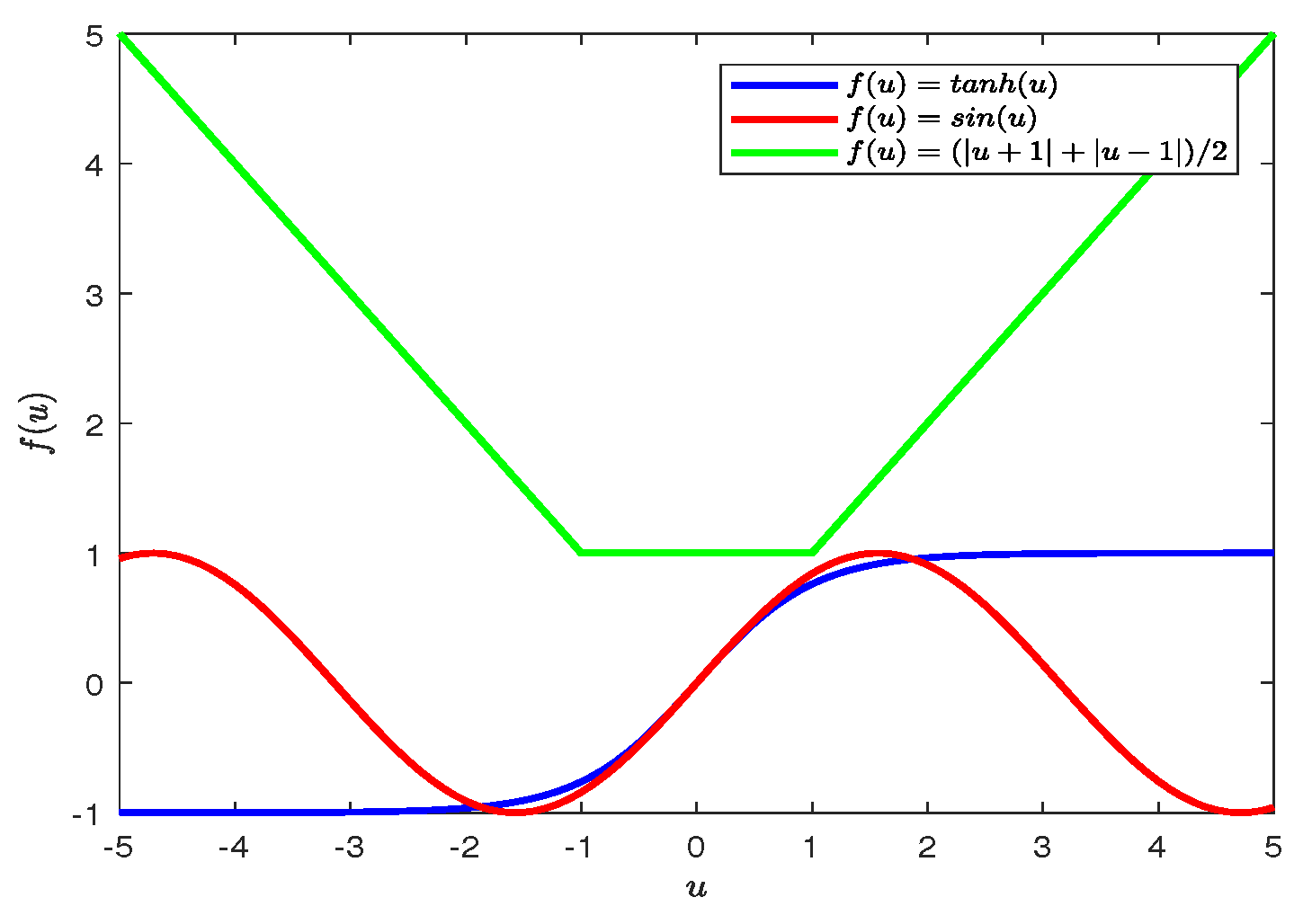
Example 1.

Consider 4-node DCDNs with R–Ds (the topology of the network is shown in Figure 1), where each node represents a delayed reaction–diffusion network:

$$\begin{array}{cc}\hfill \frac{\partial u_o(y,t)}{\partial t}=& \sum _{j=1}^4\frac{\partial }{\partial y_j}\left(a_{oj}\frac{\partial u_o(y,t)}{\partial y_j}\right)-b_o{u}_o(y,t)+\sum _{q=1}^4{c}_{oq}{f}_q\left(u_q(y,t)\right)+I_o\hfill \\ \hfill & +\sum _{q=1}^4{d}_{oq}{g}_q\left(u_i(y,t-\tau \left(t\right))\right)+\gamma \sum _{k=1}^4{l}_{ok}(y,t)\Gamma u_k(y,t),o=1,\dots ,4,\hfill \end{array}$$

(24)

where $u_o={(u_{o1},u_{o2},u_{o3},u_{o4})}^T$, $A={\sum }_{j=1}^4{a}_{oj}=diag\left\{0.1,0.1,0.1,0.1\right\}$, $B=b_o=I_4$, $\gamma =12$, $f\left(u_o\right)=g\left(u_o\right)={(\tanh \left(u_{o1}\right);\tanh \left(u_{o2}\right);\tanh \left(u_{o3}\right);\tanh \left(u_{o4}\right))}^T$. $y\in \beth =\left\{y\in \beth :|y|\le 5\right\}$, $I_{1,2,3,4}=0$, $\Gamma =1$ and

$$C=\left(\begin{array}{cccc}2.1& -0.12& 0& 0\\ -5.1& 3.2& 0& 0\\ 0& 0& 2.1& -0.12\\ 0& 0& -5.1& 3.2\end{array}\right),$$

$$D=\left(\begin{array}{cccc}-1.6& -0.1& 0& 0\\ -0.2& -2.4& 0& 0\\ 0& 0& -1.6& 0\\ 0& 0& 0& -0.1\end{array}\right).$$

Remark 7.

In contrast (in Figure 2), the gradient size of different activation functions can affect the convergence rate of the network for a given input. Therefore, we chose $f\left(u_o\right)=\tanh \left(u_o\right)$ as the activation function. $\tanh \left(u\right)$ is a smooth and continuous function, and its first derivative is continuous. This guarantees the stability and differentiability of the model. In addition, $\tanh \left(u\right)$ is a monotonically increasing function, which means that an increase in the input corresponds to an increase in the output, helping control the system. Not only that, $\tanh \left(u\right)$ is linear near zero, which helps deal with small signals and perturbations. $\sin \left(u\right)$ is a periodic function with periodic and oscillatory properties. In practical applications, this can lead to undesired periodic behavior or oscillations in the system, especially when feedback and coupling effects are included in the model, exacerbating instability. This is because $\frac{|u+1|+|u-1|}{2}$ is a piecewise linear function, continuous but not differentiable at $u=\pm 1$. This non-smoothness can lead to difficulties in numerical methods, especially in derivation and optimization. The output takes a minimum value of 0 at $u=0$ and a maximum value of 1 at $u\ge 1$. This symmetry and non-smoothness can lead to unstable behavior or numerical oscillations when dealing with complex coupled systems. Therefore, $\tanh \left(u\right)$ is selected as the activation function to ensure the stability of the model and the feasibility of the numerical solution.

Let $\widehat{\mathcal{E}}=\left\{(1,2),(1,3),(3,4),(4,2)\right\}$. Obviously, network (24) is linked by edge $\widehat{\mathcal{E}}$.

Choose ${\delta }_{ok}=2.5$ for $(o,k)\in \widehat{\mathcal{E}}$. Then, system (24) can achieve asymptotic synchronization under edge-based adaptive pinning control law (6) and (7). Let the initial value be $u_1(y,t)=\sin (\frac{1}{2}\pi +\frac{1}{8}\pi y),u_2(y,t)=-\cos \left(\frac{1}{8}\pi y\right),u_3(y,t)=-\sin (\frac{1}{2}\pi +\frac{1}{8}\pi y),u_4(y,t)=2\cos \left(\frac{1}{8}\pi y\right)$ for $t\in (-\infty ,0]$. ${\tau }_1\left(t\right)=0.02t,{\tau }_2\left(t\right)=0.04t,{\tau }_3\left(t\right)=0.01t,{\tau }_4\left(t\right)=0.06t$. 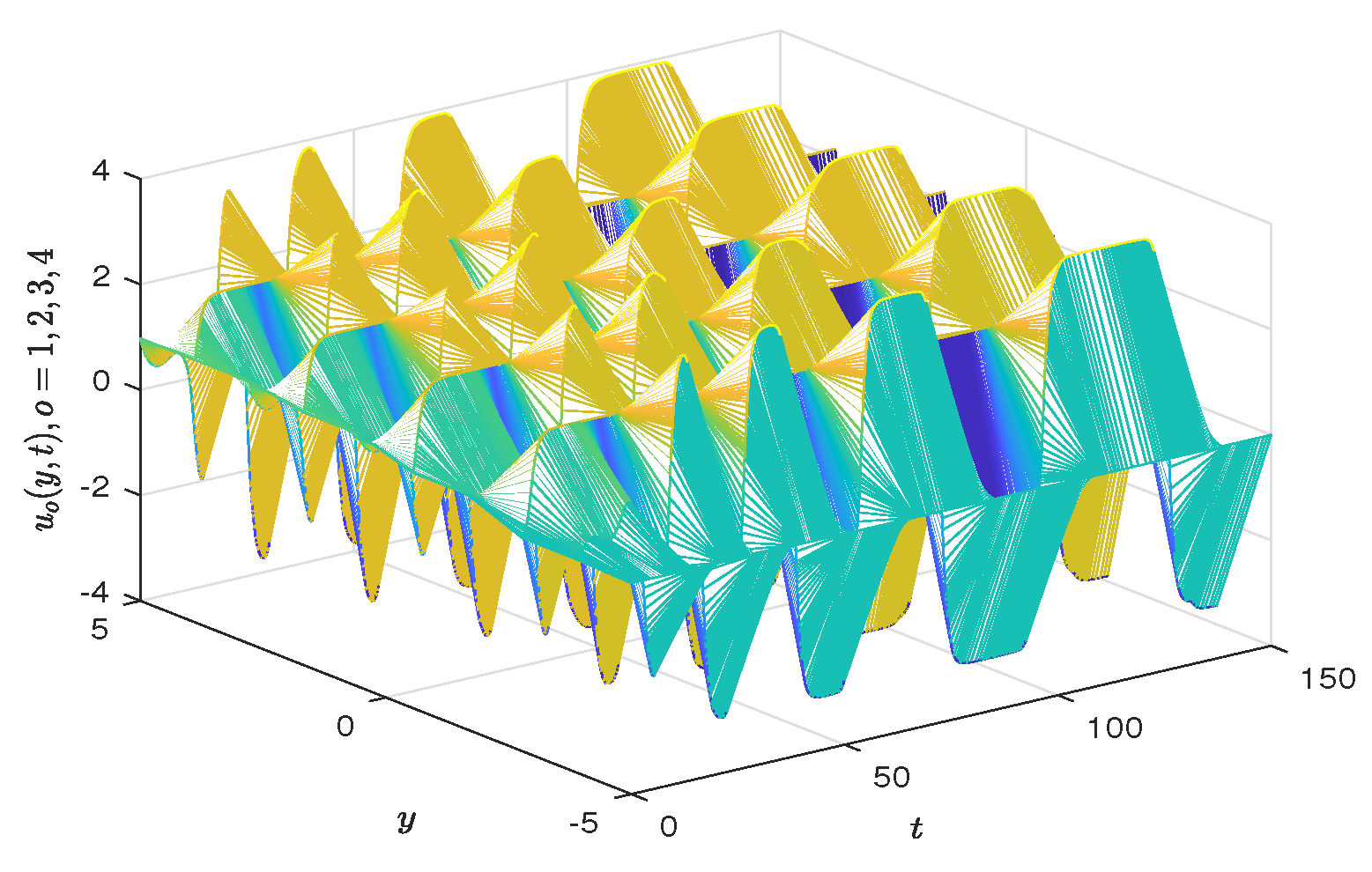Figure 3 and Figure 4 show the unstable behavior of system (24). Further, by analyzing the dynamical behavior of each node of the reaction–diffusion system (24), each node represents a reaction–diffusion system, as shown in Figure 5. Figure 6 shows the adaptive weight ($l_{ok}(y,t)$) evolution state of our pinning edge ($\widehat{\mathcal{E}}=\left\{(1,2)\right\}$), which synchronizes the whole network by pinning one of the edge and combining the coupling effect of the network. 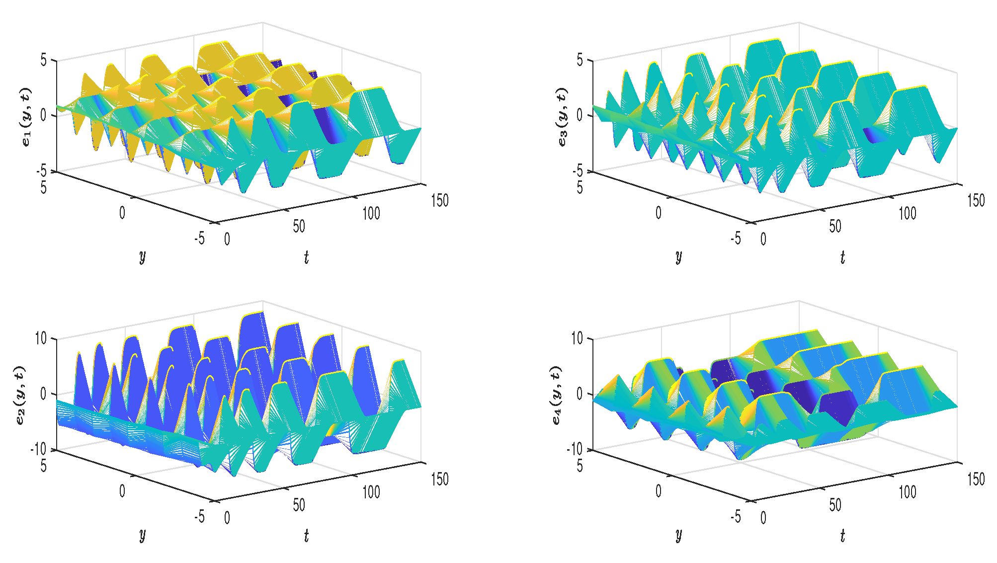Figure 7 shows the stable evolution states of the four nodes selected by the error system ($e_o(y,t),o=1,2,3,4$). Figure 8 shows that when the system is synchronized, the adaptive coupling weight of the system converges to a specific value.

Remark 8.

It should be noted that network synchronization can be achieved as long as one edge is selected, and the choice of this edge is arbitrary.

Remark 9.

(1) Matrix A on behalf of the diffusion coefficient in the reaction diffusion network. The diagonal matrix form is chosen here, and the diffusion coefficient of each node is $0.1$, which helps maintain the stability of the system. (2) The matrix B represents the dissipation coefficient in the R–D network. Choosing the identity matrix $I_4$ indicates that each node has the same dissipative term coefficient, which helps balance the energy of the system. (3) Parameter γ is an important parameter for controlling the network synchronization speed, and a larger value of γ can speed up the convergence speed of network synchronization. (4). The matrix C and D represent the coupling weights between nodes in the network. By adjusting these weights, the coupling intensity and direction between network nodes can be affected, and then the synchronization property of the network can be affected. (5) Select the edge control parameter ${\delta }_{ok}=2.5$, which is based on the requirements of the edge control policy to control the synchronization behavior of a specific edge.

Remark 10.

In Example 2, the Robin boundary condition combines the characteristics of the Dirichlet and Neumann boundary conditions, so it has certain applicability in practical problems, and can effectively cope with the complexity and diversity of the system, and can achieve synchronization and coordination among the network nodes.

Example 2.

Similarly to Example 1, choose a network model with 4-nodes in (24). The Robin boundary conditions are of the following form,

$$\begin{array}{c}\hfill {\omega }_{o1}\frac{\partial e_o(y,t)}{\partial y}+{\omega }_{o2}{e}_o(y,t)=0,o=1,2,3,4.\end{array}$$

Choose ${\omega }_{o1}=0.5,{\omega }_{o2}=0.5$. Under the Robin boundary condition, the stable state of each node of system (24) is shown in Figure 9, and Figure 10 shows the evolution state of the system after the pinning edge.

Remark 11.

In Examples 1 and 2, 4-node are selected to describe the synchronization state of the network. The model contains time delays and R–Ds. It should be noted that the effect of time delays is ignored in [18,20], and R–Ds are not considered in [7,12,13]. At the same time, the edge structure of the network diagram is used in the control method, which combines adaptive control [26,32,34] and pinning control [4,11,20]. In addition, different boundary conditions are discussed to more truly reflect the real network.

Example 3.

In order to fully verify the conclusion of this paper, a topology diagram with five nodes is considered (Figure 11).

Take $r=N=5$ in (1). $\gamma =12$, $A={\sum }_{j=1}^5{a}_{oj}=diag\left\{1,1,1,1,1\right\}$, $B=b_o=I_5$, $f\left(u_o\right)=g\left(u_o\right)={(\tanh \left(u_{o1}\right);\tanh \left(u_{o2}\right);\tanh \left(u_{o3}\right);\tanh \left(u_{o4}\right);\tanh \left(u_{o5}\right))}^T$. $y\in \beth =\left\{y\in \beth :|y|\le 5\right\}$, $I_{1,2,3,4,5}=0$, $\Gamma =1$ and

$$C=\left(\begin{array}{ccccc}2.1& -0.12& 0& 0& 0\\ -5.1& 3.2& 0& 0& 0\\ 0& 0& 2.1& -0.12& 0\\ 0& 0& -5.1& 3.2& 0\\ 0& 0& 0& 0& 1\end{array}\right),$$

$$D=\left(\begin{array}{ccccc}-1.6& -0.1& 0& 0& 0\\ -0.2& -2.4& 0& 0& 0\\ 0& 0& -1.6& 0& 0\\ 0& 0& 0& -0.1& 0\\ 0& 0& 0& 0& -2.4\end{array}\right).$$

The selection of the remaining edges and parameters is similar to Example 1 and is omitted here.

Then, the dynamic trajectory displayed by the original system (1) is shown in Figure 12. Figure 13 shows the synchronization trajectory state of the error network (5) under control laws (6) and (7). Similarly, Figure 14 shows that the adaptive coupling weight of the system converges to a specific value.

Remark 12.

Examples 1 and 3 compare different topologies, and the theoretical and simulation results show that the network can be synchronized, regardless of whether the network nodes are odd or even.

5. Conclusions

In this paper, the edge-based asymptotic synchronization of DCDNs with R–Ds is investigated. A new edge-based adaptive pinning control method is introduced, which combines the advantages of adaptive control and pinning control, and realizes network synchronization by using the coupling effect of network edge. The sufficient conditions for the synchronization of R–D networks are provided by means of Green’s formula, Wirtinger inequality, inequality analysis methods, and contradiction analysis methods. The results show that the network synchronization can be achieved by pinning one edge of the network, and the choice of edge is arbitrary, which greatly reduces the difficulty of control and is more applicable in the actual networks. Finally, a series of numerical examples are provided to illustrate the theoretical results.

At present, random factors are everywhere in the real network, and the study of random systems has become a research hotspot. Whether CDN synchronization with random interference can be realized through edge-based adaptive pinning control is a problem of great concern. I believe this is a challenging and interesting topic, and is one of our future research focuses.