Abstract
In this paper, we study the improved block splitting (IBS) iteration method and its accelerated variant, the accelerated improved block splitting (AIBS) iteration method, for solving linear systems of equations stemming from the discretization of the complex Helmholtz equation. We conduct a comprehensive convergence analysis and derive optimal iteration parameters aimed at minimizing the spectral radius of the iteration matrix. Through numerical experiments, we validate the efficiency of both iteration methods.
Keywords:
complex Helmholtz equation; complex linear system; iteration method; optimal parameter; convergence MSC:
65F08; 65F10; 65N12
1. Introduction
In this paper, we consider the complex partial differential Equation (PDE) governing the 2D field variable :
where, importantly, the parameter is a complex-valued constant. The PDE in (1) will then be referred to as the complex Helmholtz equation. The complex Helmholtz equation arises in periodically forced systems, ranging from electrochemical impedance spectroscopy to unsteady slow viscous flows, and in a broad area that has become known as diffusion wave field theory []. Discretizations of the complex Helmholtz Equation (1) using, e.g., finite differences [,,], finite element [,], or spectral element methods [], and appropriate boundary conditions result in a large, sparse, possibly complex-valued, and highly indefinite linear system:
where are symmetric positive semi-definite matrices with at least one of them being positive definite, , and is the imaginary unit. The above linear system is also widely used in scientific computing and engineering applications, such as electromagnetism, wave propagation, quantum mechanics, molecular scattering, and structural dynamics (see [,,,,,,]).
To solve the complex linear system (2), we often transform it into the following equivalent real block two-by-two form:
where , , u, v, f, , . In this paper, denotes the conjugate transpose of a matrix or a vector, denotes the transpose of a matrix or a vector, and denotes the spectral radius of a matrix, respectively.
For solving complex symmetric linear systems, a lot of iteration methods, including stationary iteration methods and Krylov subspace iteration methods (often using preconditioners) have been proposed in the literature. In this paper, we are concerned with block splitting iteration methods with parameter acceleration. In recent years, many authors have developed the block splitting iteration methods for solving complex symmetric linear systems. In 2013, for solving the real-valued linear system (3), Bai [] established a class of rotated block triangular preconditioners, and analyzed the eigenproperties of the corresponding preconditioned matrices. Following this, Salkuyeh et al. [] discussed the generalized successive overrelaxation (GSOR) iteration method in 2014, with convergence analysis. Then, to improve the convergence speed of GSOR, in 2015, Edalatpour et al. [] proposed an accelerated GSOR (AGSOR) iteration method with two parameters, and determined the optimal parameters. In 2018, Li et al. [] constructed a symmetric block triangular splitting (SBTS) iteration method based on two splittings, and gave the convergence conditions as well as the optimal parameters. In 2019, Axelsson and Salkuyeh [] derived the transformed matrix iteration (TMIT) method and gave the convergence conditions; they also determined that the optimal parameter of TMIT method was contained in the interval . In 2021, Siahkolaei et al. [] gave an upper bound for the spectral radius of the iteration matrix of the TMIT method and then obtained the parameter which minimizes this upper bound.
Recently, Huang [] studied a new block splitting (NBS) iteration method and a parameterized block splitting (PBS) iteration method to solve the real value linear system (3). In this paper, we continue to study BS iteration methods for solving (3). We will construct the improved block splitting (IBS) iteration method and give the corresponding convergence analysis. Furthermore, using the parameter accelerating technique for the IBS iteration method, we will construct the accelerated improved block splitting (AIBS) iteration method based on the split of the AGSOR iteration method.
The remainder of this paper is organized as follows. In Section 2, we construct the IBS iteration method to solve the linear system with a real value (3) and give the convergence analysis. In Section 3, we study the AIBS iteration method and give the convergence analysis. In Section 4, we present some numerical examples to demonstrate the effectiveness of the IBS and AIBS iteration methods. Finally, some conclusions are drawn in Section 5.
2. IBS Iteration Method and Its Convergence Analysis
In this section, we study the IBS iteration method for solving the real-valued linear system (3). First, we recall the NBS and PBS iteration methods. Multiply both sides of (3) from the left by the block matrix:
where is a positive constant, and denote:
where d, . Then, (3) can be written as:
Split the coefficient matrix of (6) as follows:
Then, it yields the following NBS iteration:
where the iteration matrix is:
To derive the PBS method, we multiply both sides of (3) from the left by the matrix P in (4) and denote:
where is a positive constant and . Then, (3) can be written as:
Remark 1.
For the NBS method, the optimal parameter , which minimizes the upper bound of the spectral radius is , see Theorem 2.1 in []. Furthermore, for the PBS method, maybe not optimal, the parameter is still taken as , see Theorem 3.2 in [].
By the idea of NBS and PBS methods, we take the parameter directly, then (6) can be written as:
Split the coefficient matrix of (14) as follows:
where is a positive constant. Then, it yields the following IBS iteration:
where the iteration matrix is:
IBS iteration algorithm: Given initial vectors , for until the sequence converges, compute:
From the iteration scheme (18), it can be seen that two linear subsystems with respect to the symmetric positive definite coefficient matrix need to be solved at each iteration step. It can be solved by Cholesky factorization [].
Next, we give the convergence analysis for the IBS method, and discuss the optimal parameter that minimizes the spectral radius .
Theorem 2.
Let W be symmetric positive definite and T be symmetric positive semi-definite, respectively, and . Then:
- (1)
- The eigenvalues of the iteration matrix are taken as follows:where are the eigenvalues of the matrix .
- (2)
- if and only if α satisfies the following conditions:
- (a)
- If :
- (b)
- If :
- (c)
- If , , then:
- (3)
- has the following expression:(a) If or :(b) If , , then:where
Proof.
Let:
Then, by the Equation , the following holds:
That is, is similar to the following matrix :
in which . Then, and have the same eigenvalues. Let be the eigendecomposition of S, where is an orthogonal matrix, , and Z denotes transpose in this paper. Denote:
and . Then, it holds that:
Notice that , and have the same eigenvalues, and is a diagonal matrix with the main diagonal elements being , . Then, it is easy to see that the eigenvalues of are:
Hence, the conclusion (1) is proved.
Next, we prove conclusion (2). By the Equation , it holds that:
Notice for any , holds obviously. Now, we consider the solution to , i.e., . Define , . Then, the derivative of is . We discuss the following three cases:
- (a)
- If , then , i.e., is monotonically decreasing with respect to u, which means , so ;
- (b)
- If , then , i.e., is monotonically increasing with respect to u, which means , so ;
- (c)
- If , then is monotonically decreasing in and monotonically increasing in , respectively, so it holds that , which yields .
Hence, conclusion (2) is proved.
Next, we prove the conclusion (3). Define , , then we have . We discuss the following two cases:
- (a)
- If , then , is monotonically increasing, and it is easy to see that:Similarly, when , is monotonically decreasing, then has the same form of .
- (b)
- If , then is monotonically increasing in and monotonically decreasing in , respectively. In this case has maximum . Then, we consider the following two cases.
Cases I: When , i.e., , then we have:
Cases II: When , i.e., , then we consider the following two subcases.
If , then . When , then . When , then . Thus, we have:
If , then . When , then . When , then . Thus, we have:
Then, it holds by the above discussion that:
where
which finishes the proof. □
Theorem 2 gives the convergence conditions for the IBS method. Now, we investigate the optimal parameter that minimizes .
Theorem 3.
Assume that the conditions of Theorem 2 are satisfied and are the eigenvalues of . Then, the optimal parameter which minimizes and the corresponding optimal convergence factor are given by:
- (1)
- If or , then:
- (2)
- If , , then:where
Proof.
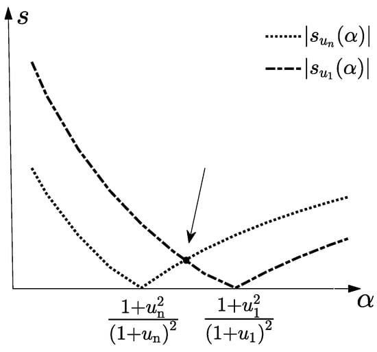
(1) If , then:
Define , then . Notice , then is monotonically increasing with respect to , and is monotonically decreasing with respect to . As shown in Figure 1, the arrow points to the position of the optimal parameter, and it is easy to see that the optimal satisfies: , and after some algebra we have .
Figure 1.
The image of , where .
Substitute into we have:
Similarly, if , has the same expression as . Substitute into we have:
(2) If , let then:
where
Notice is monotonically increasing with respect to and is monotonically decreasing with respect to . We now discuss the following two cases:
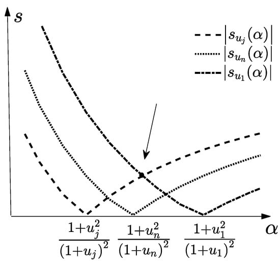
When , then , i.e., :
As shown in Figure 2, the image of is above the image of , and the arrow points to the position of the optimal parameter , and it is easy to see the optimal satisfies , after some algebra we have . Substitute into , we have:
Figure 2.
The image of , where .
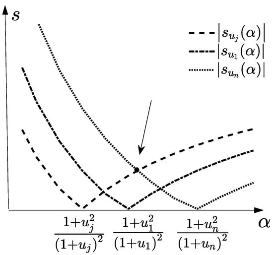
When , then , i.e., .
As shown in Figure 3, the image of is above the image of , and the arrow points to the position of the optimal parameter, and the optimal satisfies , after some algebra, we have . Substitute into we have:
which finishes the proof. □
Figure 3.
The image of , where .
Remark 4.
From Theorem 3 we see that if , , then:
However, generally it is very expensive to compute and that satisfies . In our numerical experiments, when , we approximate by taking , which yields the following practical optimal parameter:
3. AIBS Iteration Method and Its Convergence Analysis
In this section, inspired by the idea of the AGSOR iteration method, we construct the AIBS iteration method, which generalizes the IBS one and has faster convergence speed.
First, we recall the AGSOR iteration method. Multiplying both sides of from the left by the block matrix:
where is a positive constant and I is the identity matrix, then can be written as:
Split the coefficient matrix of (35) as follows:
Then, it yields the AGSOR iteration, whose iteration matrix is:
Now we construct the AIBS iteration method, which is just a preconditioned AGSOR (PAGSOR) iteration method. Recall in Section 2; the linear system can be written by the following form:
Multiplying both sides of from the left by the matrix , we have:
Similar to AGSOR, split the coefficient matrix of (37) as follows:
Then, it yields the following AIBS (PAGSOR) iteration:
where the iteration matrix is:
AIBS iteration algorithm: Given initial vectors , for until the sequence converges, compute:
Remark 5.
The IBS iteration method is the special case of the AIBS one as , since they have the same iteration matrix when .
Next, we discuss the convergence properties of the AIBS iteration method.
Lemma 1
([]). Both roots of the real quadratic equation are less than one in the modulus if and only if and .
Lemma 2.
Let W be symmetric positive definite and T be symmetric positive semi-definite, respectively, and are the eigenvalues of . Let , . Then, the maximum and the minimum of satisfy the following equations:
Proof.
Define , , then we have . We now discuss the following three cases:
- (1)
- If , then , i.e., is monotonically increasing with respect to u:
- (2)
- If , then , i.e., is monotonically decreasing with respect to u:
- (3)
- If , then is monotonically increasing and monotonically decreasing in and , respectively:
□
Remark 6.
In Lemma 2, when , , then . Since it is difficult to compute a and that satisfy , in our numerical experiments, when , we take , which is equivalent to or .
Theorem 7.
Assume that the conditions of Lemma 2 are satisfied. Then, the AIBS iteration method is convergent if the parameters α and β satisfy:
where , .
Proof.
Let:
Then, by Equation , it holds that:
where
That is, is similar to the following matrix :
in which . Then, and have the same eigenvalues. Let be the eigendecomposition of S, where is an orthogonal matrix, . Denote:
and . Then, it holds that:
Notice that the non-zero block matrices of are all diagonal matrices; define:
then it is easy to see that:
The eigenvalues of the matrix satisfy the following equation:
Let:
Then, (41) can be written as:
Now, by Lemma 1, if and only if:
Solving the above inequality yields:
Noticing is monotonically increasing with respect to , we have:
which finishes the proof. □
Remark 8.
Theorem 7 gives the convergence conditions for the AIBS iteration method. Now, we discuss the optimal parameters and which minimize . It is very sophisticated when , so in this paper and for this problem, we assume . Together with the convergence conditions in Theorem 7, we now assume to investigate the local optimal parameters.
Theorem 9.
Assume that the conditions of Lemma 2 are satisfied, and , where , . Then, the optimal parameters and which minimize are given by:
where
and the corresponding optimal convergence factor is given by:
Proof.
The two roots of (42) are given by:
where
Let be the larger modulus of the two roots and , that is:
Then, we discuss the following two cases.
- (1)
- If , then:that is:
- (2)
- If , then and are real, and it holds that:Denote , then the spectral radius of the AIBS iteration matrix can be defined by:Let:Then, it holds that:When and , i.e., , then:When and , i.e., , then:After some algebra, we have when and , then:when and , then:It is easy to see there exist two variables , satisfying the following equations:Now, we prove . Define , , is monotonically increasing with respect to . If , then we have , that is:by (45) and (47), it holds that:which means , then it contradicts ; If , then , that is:by (46) and (48), it holds that:which means , then it contradicts . Hence, .Then, we have:For convenience, let , . Without loss of generality, suppose . In fact, if , , then , i.e., , which is the extreme trivial situation. It is easy to see that the following results hold true.:Then, we have:Notice:wherethen, it holds that:Analogously, it also holds that:
Similar to the proof of Theorem 2.5 in [], has a minimum at .
First, we prove has no minimum at , see the following two cases.
Assume has a minimum at . By (52), it holds that , let . Then, . By the above monotone property of the function , we have , which contradicts the assumption.
Assume has minimum at . By (52), it holds that , let , then . By the above monotone property of the function , we have , which contradicts the assumption.
It is easy to see from the above two cases that may have a minimum only at .
When , from (51) and (52), it holds that:
Let , and define a function :
When , i.e., , it holds that
so and .
When , it holds that , which means is increasing with respect to t.
4. Numerical Results
In this section, we present some numerical examples to demonstrate the effectiveness of the IBS iteration method and the AIBS iteration method. All the computations are implemented in MATLAB (version R2021a) on a PC computer with 16.0 GB memory, an Intel(R) Core(TM) i5-10500 CPU @1.19 GHz, and Windows 10 as the operating system. We denote the elapsed CPU time (in second) by CPU, the iteration numbers by IT, and the norm of the relative residuals by RES, respectively. In our computations all the initial guesses are taken by zero vectors, and the computations are terminated once the stopping criterion is satisfied:
We compare the AIBS and IBS methods with NBS, PBS, AGSOR, and PMHSS methods, including the corresponding preconditioned GMRES methods. In each iteration of AIBS, IBS, NBS, PBS, AGSOR, and PMHSS methods, we use the Cholesky factorization to solve the subsystems. In addition, we use the preconditioned restarted GMRES(20) in our numerical tests. The iteration number k of GMRES means , where i is the number of restarting, and p is the iteration number of the last restarting, respectively.
Example 1.

Consider the following complex symmetric linear system Equation [,]:
where τ is the time step-size and K is the five-point centered difference matrix approximating the negative Laplacian operator with homogeneous Dirichlet boundary conditions, on a uniform mesh in the unit square with the mesh-size . The matrix possesses the tensor-product form , with . Hence, K is an block tridiagonal matrix, with . We take:
and the right-hand side vector with its th entry is given by:
Making , and multiplying both sides of the system of equations by to regularize the coefficient matrix and the right-hand side vector at the same time.
Table 1 lists the optimal parameters for the AIBS, IBS, PBS [], NBS [], AGSOR [], and PMHSS [] methods. , represents the optimal parameters for each method. Table 2 and Table 3 list the IT, CPU, and RES of each iteration method for Example 1.
Table 1.
The optimal parameters for Example 1.
Table 2.
Numerical results of stationary iterations for Example 1.
Table 3.
Numerical results of preconditioned GMRES for Example 1.
Example 2.
Consider the following complex Helmholtz Equation [,]:
where , are real coefficient functions and u satisfies Dirichlet boundary conditions in . The above equation describes the propagation of damped time-harmonic waves. We take H the five-point centered difference matrix approximating the negative Laplacian operator on an uniform mesh with meshsize . The matrix possesses the tensor-product form , with . Hence, H is an block-tridiagonal matrix, with . This leads to the complex symmetric linear system:
In addition, we set , and the right-hand side vector to be , with 1 being the vector of all entries equal to 1. We normalize the system by multiplying both sides by .
Table 4 lists the optimal parameters for the AIBS, IBS, PBS [], NBS [], AGSOR [], and PMHSS [] methods. , represents the optimal parameters for each method. Table 5 and Table 6 list the IT, CPU, and RES of each iteration method for Example 2.
Table 4.
The optimal parameters for Example 2.
Table 5.
Numerical results of stationary iterations for Example 2.
Table 6.
Numerical results of preconditioned GMRES for Example 2.
5. Conclusions
For solving a complex symmetric linear system from the complex Helmholtz equation, based on the NBS and AGSOR iteration methods, we construct the IBS and AIBS iteration methods for solving its equivalent real-valued form. We analyze the convergence of the two iteration methods, and obtain the corresponding optimal parameters that minimize the spectral radius of the iteration matrix. It can be shown in our numerical results that, both for the stationary iteration and as a preconditioner to accelerate GMRES, IBS, and AIBS methods always outperform some existing iteration methods, such as the NBS method, PBS method, AGSOR method, PMHSS method, and so forth. The technique in this paper is valid for the 2D problem, and it can be tried to solve 3D problem, which will be our future work.
Author Contributions
Conceptualization, N.Z.; Methodology, Y.Z., N.Z. and Z.C.; Validation, Y.Z. and Z.C.; Writing—original draft, Y.Z. and N.Z.; Writing—review & editing, Z.C. All authors have read and agreed to the published version of the manuscript.
Funding
This research received no external funding.
Data Availability Statement
Data are contained within the article.
Conflicts of Interest
The authors declare no conflict of interest.
References
- Mandelis, A. Diffusion-Wave Fields: Mathematical Methods and Green Functions; Springer Science & Business Media: Berlin/Heidelberg, Germany, 2013. [Google Scholar]
- Singer, I.; Turkel, E. High-order finite difference methods for the Helmholtz equation. Comput. Methods Appl. Mech. Eng. 1998, 163, 343–358. [Google Scholar] [CrossRef]
- Wu, Z.; Alkhalifah, T. A highly accurate finite-difference method with minimum dispersion error for solving the Helmholtz equation. J. Comput. Phys. 2018, 365, 350–361. [Google Scholar] [CrossRef]
- Fu, Y. Compact fourth-order finite difference schemes for Helmholtz equation with high wave numbers. J. Comput. Math. 2008, 26, 98–111. [Google Scholar]
- Oberai, A.; Pinsky, P. A multiscale finite element method for the Helmholtz equation. Comput. Methods Appl. Mech. Eng. 1998, 154, 281–297. [Google Scholar] [CrossRef]
- Oberai, A.; Pinsky, P. A residual-based finite element method for the Helmholtz equation. Int. J. Num. Meth. Eng. 2000, 49, 399–419. [Google Scholar] [CrossRef]
- Mehdizadeh, O.; Paraschivoiu, M. Investigation of a two-dimensional spectral element method for Helmholtz’s equation. J. Comput. Phys. 2003, 189, 111–129. [Google Scholar] [CrossRef]
- Feriani, A.; Perotti, F.; Simoncini, V. Iterative system solvers for the frequency analysis of linear mechanical systems. Comput. Methods Appl. Mech. Engrg. 2000, 190, 1719–1739. [Google Scholar] [CrossRef]
- Hiptmair, R. Finite elements in computational electromagnetism. Acta Numer. 2003, 11, 237–339. [Google Scholar] [CrossRef]
- Howle, V.E.; Vavasis, S.A. An iterative method for solving complex-symmetric systems arising in electrical power modeling. SIAM J. Matrix Anal. Appl. 2005, 26, 1150–1178. [Google Scholar] [CrossRef]
- Rees, T.; Dollar, H.S.; Wathen, A.J. Optimal solvers for PDE-constrained optimization. SIAM J. Sci. Comput. 2010, 32, 271–298. [Google Scholar] [CrossRef]
- Bai, Z.-Z. Block preconditioners for elliptic PDE-constrained optimization problems. Computing 2010, 91, 379–395. [Google Scholar] [CrossRef]
- Axelsson, O.; Neytcheva, M.; Ahmad, B. A comparison of iterative methods to solve complex valued linear algebraic systems. Numer. Algor. 2014, 66, 811–841. [Google Scholar] [CrossRef]
- Benzi, M.; Bertaccini, D. Block preconditioning of real-valued iterative algorithms for complex linear systems. IMA J. Numer. Anal. 2008, 28, 598–618. [Google Scholar] [CrossRef]
- Bai, Z.-Z. Rotated block triangular preconditioning based on PMHSS. Sci. China Math. 2013, 56, 2523–2538. [Google Scholar] [CrossRef]
- Salkuyeh, D.K.; Hezari, D.; Edalatpour, V. Generalized successive overrelaxation iterative method for a class of complex symmetric linear system of equations. Int. J. Comput. Math. 2015, 92, 802–815. [Google Scholar] [CrossRef]
- Edalatpour, V.; Hezari, D.; Salkuyeh, D.K. Accelerated generalized SOR method for a class of complex systems of linear equations. Math. Commun. 2015, 20, 37–52. [Google Scholar]
- Li, X.-A.; Zhang, W.-H.; Wu, Y.-J. On symmetric block triangular splitting iteration method for a class of complex symmetric system of linear equations. Appl. Math. Lett. 2018, 79, 131–137. [Google Scholar] [CrossRef]
- Axelsson, O.; Salkuyeh, D.K. A new version of a preconditioning method for certain two-by-two block matrices with square blocks. BIT 2018, 59, 321–342. [Google Scholar] [CrossRef]
- Siahkolaei, T.S.; Salkuyeh, D.K. On the parameter selection in the transformed matrix iteration method. Numer. Algor. 2020, 86, 179–189. [Google Scholar] [CrossRef]
- Huang, Z.-G. Efficient block splitting iteration methods for solving a class of complex symmetric linear systems. J. Comput. Appl. Math. 2021, 395, 113574. [Google Scholar] [CrossRef]
- Golub, G.H.; Van Loan, C.F. Matrix Computations. In Johns Hopkins Studies in the Mathematical Science, 3rd ed.; Johns Hopkins University Press: Baltimore, MD, USA, 1996. [Google Scholar]
- Young, D.M. Iterative Solution of Large Linear Systems; Academic Press: New York, NY, USA, 1971. [Google Scholar]
- Chao, Z.; Zhang, N.-M.; Lu, Y.-Z. Optimal parameters of the generalized symmetric SOR method for augmented systems. J. Comput. Appl. Math. 2014, 266, 52–60. [Google Scholar] [CrossRef]
- Axelsson, O.; Kucherov, A. Real valued iterative methods for solving complex symmetric linear systems. Numer. Linear Algebra Appl. 2000, 7, 197–218. [Google Scholar] [CrossRef]
- Bai, Z.-Z.; Benzi, M.; Chen, F. Modified HSS iteration methods for a class of complex symmetric linear systems. Computing 2010, 87, 93–111. [Google Scholar] [CrossRef]
- Bai, Z.-Z.; Benzi, M.; Chen, F. Preconditioned MHSS iteration methods for a class of block two-by-two linear systems with applications to distributed control problems. IMA J. Numer. Anal. 2013, 33, 343–369. [Google Scholar] [CrossRef]
- Bertaccini, D. Efficient preconditioning for sequences of parametric complex symmetric linear systems. Electron. Tran. Numer. Anal. 2004, 18, 49–64. [Google Scholar]
- Li, X.; Yang, A.-L.; Wu, Y.-J. Lopsided PMHSS iteration method for a class of complex symmetric linear systems. Numer. Algor. 2014, 66, 555–568. [Google Scholar] [CrossRef]
Disclaimer/Publisher’s Note: The statements, opinions and data contained in all publications are solely those of the individual author(s) and contributor(s) and not of MDPI and/or the editor(s). MDPI and/or the editor(s) disclaim responsibility for any injury to people or property resulting from any ideas, methods, instructions or products referred to in the content. |
© 2024 by the authors. Licensee MDPI, Basel, Switzerland. This article is an open access article distributed under the terms and conditions of the Creative Commons Attribution (CC BY) license (https://creativecommons.org/licenses/by/4.0/).