An Agile Adaptive Biased-Randomized Discrete-Event Heuristic for the Resource-Constrained Project Scheduling Problem

Abstract

In industries such as aircraft or train manufacturing, large-scale manufacturing companies often manage several complex projects. Each of these projects includes multiple tasks that share a set of limited resources. Typically, these tasks are also subject to time dependencies among them. One frequent goal in these scenarios is to minimize the makespan, or total time required to complete all the tasks within the entire project. Decisions revolve around scheduling these tasks, determining the sequence in which they are processed, and allocating shared resources to optimize efficiency while respecting the time dependencies among tasks. This problem is known in the scientific literature as the Resource-Constrained Project Scheduling Problem (RCPSP). Being an NP-hard problem with time dependencies and resource constraints, several optimization algorithms have already been proposed to tackle the RCPSP. In this paper, a novel discrete-event heuristic is introduced and later extended into an agile biased-randomized algorithm complemented with an adaptive capability to tune the parameters of the algorithm. The results underscore the effectiveness of the algorithm in finding competitive solutions for this problem within short computing times.

1. Introduction

Large-scale manufacturing companies often manage several complex projects, each of them containing many tasks that are affected by time-precedence relations and share resources among them. Hence, scheduling projects in assembly lines represents a relevant and challenging problem to solve for company managers. This project scheduling problem, known in the literature as the Resource Constrained Project Scheduling Problem (RCPSP), has been extensively studied in construction, manufacturing, aerospace, and other various industries [1]. One of the most frequent objectives of the RCPSP is to minimize the project’s total duration (makespan) by scheduling the tasks under the constraints of task precedence relations and resource availabilities. The RCPSP has been proven to be NP-Hard [2], which makes it more challenging as the number of tasks increases. This poses a challenging problem to solve for large-scale companies with massive projects.

Project scheduling can be categorized based on various factors, including the approach employed (dynamic or static), the consideration of uncertainty (stochastic or deterministic), and the inclusion of resource transfer time. Among others Krüger and Scholl [3] and Lu et al. [4] address this variant of the problem which is named RCPSP with Resource Transfer Time [5]. The purpose of imposing minimal time lags is to account for certain practical considerations and real-world constraints. It acknowledges that there are often logistical factors, resource setup times, or physical limitations that prevent immediate transitions between tasks. These time lags can be necessary to allow for equipment setup, cleaning, maintenance, or other operational requirements. Furthermore, the literature also distinguishes between single-project and multi-project scenarios. Kurtulus and Narula [6] introduced the multi-project approach to the scheduling problem proposing and comparing different priority rules. Multi-project scenarios are characterized by the coexistence of different projects with their associated tasks and the objective is minimizing the overall mean completion time. In multi-project scenarios, each project can have a due date and a penalty associated with delays [7]. Unlike the single-project approach, which merges all projects into one large project, and usually aims at minimizing the end time of the last task.

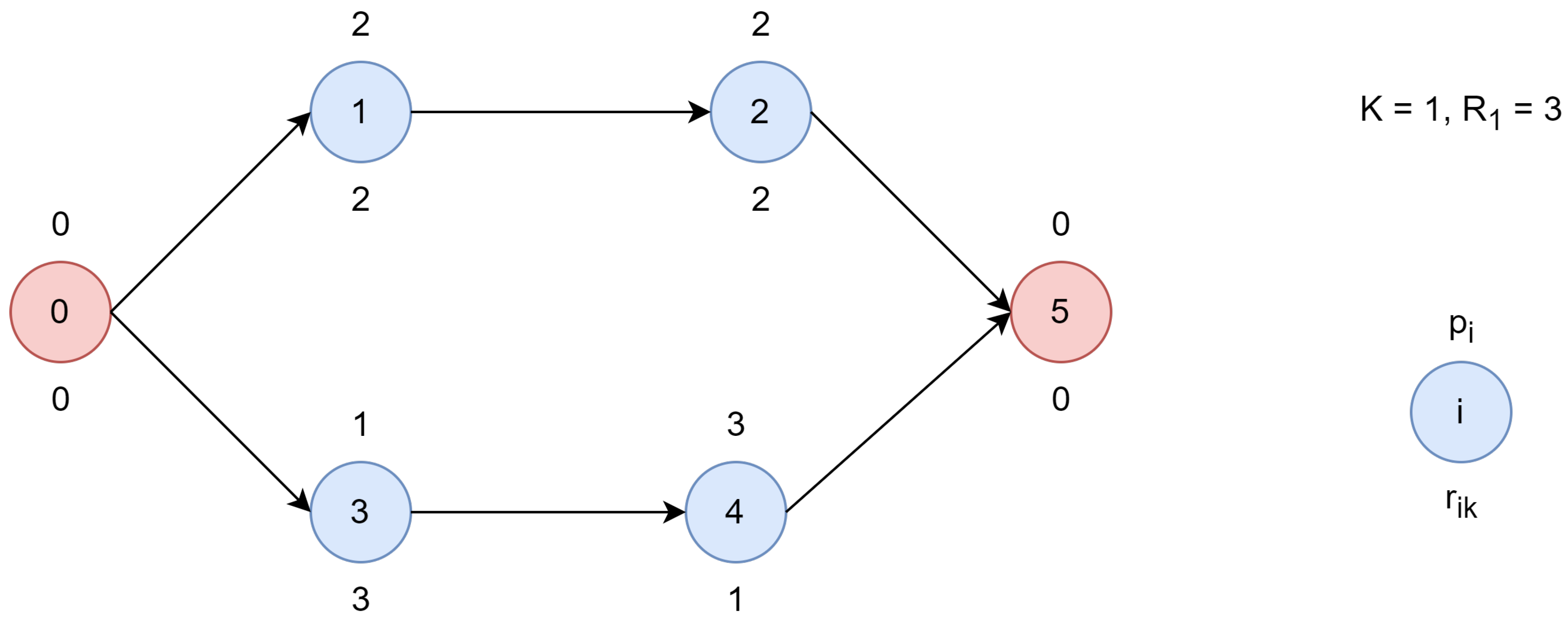
In the RCPSP, a project consists of various tasks or activities that need to be scheduled to complete the project. Each task has a defined duration and requires specific resources for completion. Certain tasks may depend on the completion of others, establishing precedence relations that define the order in which tasks must be executed. Resources necessary for performing tasks are limited in quantity, such as labor availability, equipment availability, budget constraints, or other scarce resources. The classical RCPSP formulation is based on a directed acyclic graph, where nodes represent tasks and arcs symbolize precedence relations. Tasks have start and finish times and consume a certain amount of finite capacity resources. In essence, this problem considers resources that can be shared among multiple tasks but have limitations on their simultaneous usage. For example, a specific piece of equipment or a specialized tool may have limited availability. Once allocated to a task, it cannot be used elsewhere until it becomes available again. The problem entails finding an assignment of start times to tasks so that the makespan is minimized while the following constraints are satisfied: (i) no resource capacity is exceeded at any point in time, and (ii) time dependencies among tasks are respected.

A simple but illustrative example is presented in Figure 1. It belongs to a project with four tasks (represented by blue circles). Hence, the task list contains six elements, including the start and finish dummy tasks (represented by red circles) that have been added to signal the start and end of the project, i.e., $V=\{0,1,2,3,4,5\}$. In this case, only one resource ($K=1$) is considered with a maximum availability of three units at a time ($R_1=3$). For each task i, its duration ($p_i$) is assumed to be constant and is represented by a number over the task node. For each task i, its associated resource requirement ($r_{ik}$) is included below the task node. The graph representation provides information about the precedence relationships. For instance, task 1 and task 3 can start immediately as they are direct successors of the dummy task 0. Conversely, task 2, as a direct successor of task 1, must start after task 1. This relationship is shown with a directed arc from task 1 to task 2. Similar reasoning applies to the relationship between tasks 3 and 4. Finally, the time taken between tasks 2 and 4, versus task 5 (which is the dummy task indicating the end of the project), is equal to the duration of those tasks since the project is not considered completed until the direct predecessors of the dummy end task are finished. Figure 2 shows a potential schedule for this problem. Numbers inside each blue rectangle represent tasks, which have to satisfy precedence relationships over time. The horizontal size of each rectangle represents the task duration, while the vertical size represents the use of resource $R_1$ units.

This work proposes a novel agile biased-randomized (BR) discrete-event heuristic (DEH) to efficiently address the RCPSP within short computational times. On the one hand, BR is a technique that allows the transformation of a constructive heuristic into a probabilistic algorithm without losing the logic behind the heuristic [8]. On the other hand, DEH makes use of a heuristic procedure that is driven by a discrete-event list in order to account for time dependencies in a natural way [9]. This hybrid BR and DEH approach is extended with an adaptive self-learning mechanism designed to tune the algorithm’s parameters without necessitating prior analysis or incurring expensive computational costs. Consequently, the primary contributions of this paper can be summarized as follows: (i) It introduces a novel DEH capable of providing reasonably good solutions to the RCPSP in real-time (less than a second even for the largest instances tested in this paper); (ii) it extends the previous DEH into an agile BR-DEH algorithm [10], which demonstrates its capability to produce state-of-the-art results within short computational times (some seconds of computing time) and (iii) it supplements the aforementioned BR-DEH algorithm with a self-learning mechanism to dynamically adjust associated parameters during execution. It is observed that discrete-event heuristics have proven highly effective in practical applications involving problems with time-based dependencies and constraints [9,11]. To the best of our knowledge, this is the first time in which a DEH algorithm has been utilized and combined with BR techniques to efficiently solve the RCPSP.

The remainder of this work is structured as follows: Section 2 reviews the recent literature on the RCPSP. The mathematical model formulation is presented in Section 3. Section 4 describes the novel BR-DEH algorithm introduced to solve the RCPSP. The computational experiments performed to test the proposed methodology are detailed in Section 5, while the obtained results are analyzed and discussed in Section 6. Lastly, Section 7 presents the conclusions and discusses future work.

2. Related Work

The RCPSP has been extensively studied in numerous research papers, a comprehensive survey of this problem and its variants can be found in Hartmann and Briskorn [12] and Sánchez et al. [7]. This problem can be categorized across various fields of research, such as dynamic versus static approaches, stochastic versus deterministic considerations, and the inclusion or exclusion of resource transfer time. Additionally, the literature distinguishes between single-project and multi-project scenarios. Most literature proposing solutions to this problem implements their algorithms using a standard set of instances established by Rainer and Arno [13]. These instances serve as reference benchmarks, enabling performance evaluation and comparison across different approaches. A set of summary measures for evaluating algorithm performance and analyzing instances and datasets related to the RCPSP can be found in Van Eynde et al. [14]. Consequently, a benchmark for the multi-project version of the problem is available in Van Eynde and Vanhoucke [15].

Static multi-project approaches pertain to scenarios where the number of projects remains fixed, and a schedule is developed assuming no additional projects are incorporated. Conversely, dynamic approaches apply to situations where new projects can be added to the existing portfolio, consequently altering the schedule’s sequence. Pioneering authors in the static approach include Pritsker et al. [16], who introduced a computationally tractable mathematical formulation dealing with diverse constraints and cost functions to be optimized. Kurtulus and Narula [6] introduced the multi-project approach, comparing different priority rules and aiming to minimize the overall mean completion time. Several studies have addressed the multi-project RCPSP, including works by Hartmann and Briskorn [17], Kolisch and Hartmann [18], which present surveys of heuristic approaches by different authors. The single-project approach amalgamates all projects into one, aiming to minimize the end time of the last project. Authors like Herroelen et al. [19] presented comprehensive surveys of various approaches in both single and multi-project versions.

Several recent papers, such as Pellerin et al. [20], have provided reviews focusing on hybrid heuristics, as also observed in works by Blum et al. [21], Talbi [22], and Lozano and García-Martínez [23]. These studies explain different hybrid heuristic flavors and present their application results on the PSPLIB set of instances. The differentiation between stochastic and deterministic RCPSP is outlined in Herroelen and Leus [24], discussing five scheduling scenarios. Reactive or deterministic approaches assume fixed task completion and resource transfer times without any uncertainty. Stochastic or proactive approaches develop schedules considering uncertainties in these times, aiming for robustness against potential project disruptions. Trying to find near-optimal solutions, Proon and Jin [25] proposed a genetic algorithm coupled with a neighborhood local search strategy, demonstrating competitive results compared to state-of-the-art solutions across numerous PSPLIB instances [13]. Similarly, Lim et al. [26] proposed an annealing-like search heuristic enhanced by a genetic algorithm framework, displaying competitive results among the best in the literature. Likewise, Etminaniesfahani et al. [27] introduced a relax-and-solve algorithm using CPLEX CP, which showed competitiveness and produced results comparable to [25]. Additionally, Berthaut et al. [28] implemented a path-relinking-based algorithm combining path-relinking and scatter search techniques. A study on the automatic detection of the most effective priority rule is explored by Guo et al. [29]. Their approach demonstrated superior solution quality and computation time when compared to existing methods, indicating its potential as a promising solution for the RCPSP. Recently, Hua et al. [30] introduced an improved genetic algorithm that employs time window decomposition, enhancing population diversity through three derivation methods and optimizing search efficiency with a novel sampling count allocation strategy and destructive lower bounds. This method has demonstrated superior performance in computational experiments on PSPLIB, showcasing its potential in evolutionary algorithm research for RCPSP. Golab et al. [31] proposed a convolutional neural network (CNN) approach that bypasses the need for generating multiple solutions or populations, instead using an evolved CNN within a serial schedule generation scheme to effectively prioritize project activities. Liu et al. [32] presented a straightforward algorithm combining the “1 + 1” evolution strategy with a genetic algorithm framework, which innovatively eliminates parameter tuning and employs real-valued numbers and path representation. This method proved competitive against benchmark algorithms, though further research is needed to enhance its exploration capabilities. Lastly, Pérez Armas et al. [33] explored the conversion of Mixed Integer Linear Programming formulations into a Quadratic Unconstrained Binary Optimization model, solvable via the D-Wave Advantage Quantum Annealing machine. This approach yielded promising results, particularly for smaller to medium-sized instances, demonstrating the potential of quantum computing in RCPSP solutions. Together, these studies highlight the expanding frontier of RCPSP research, driven by a blend of classical, evolutionary, and quantum computing methodologies. Apart from the basic RCPSP, recent work focuses on designing robust solutions that can take into account uncertainty in the duration of tasks [34], projects with a flexible structure [35], use of deep reinforcement learning to address resource disruptions [36], realistic projects with multiple objectives [37,38], etc.

3. Problem Description

An RCPSP instance consists of a set $V=\{0,1,\dots ,n,n+1\}$ of tasks. For each task $j\in V$, a duration or processing time $d_j$ is known, and it is assumed to be deterministic and integer-valued. Tasks 0 and n + 1 are dummy tasks representing the start and the end of the project, respectively, and have zero processing time and do not consume resources. Clearly, there are precedence relations between tasks. For each task j, a set $P_j$ is defined, containing all its predecessors. Task j can only start after all its predecessors have completed. Preemption is not permitted, i.e., tasks are executed continuously for $d_j$ time periods from their start time without interruption. Notice that V and P form a directed acyclic graph where V is the node-set, and $P_j$ determines the set of preceding nodes that have an input arc to the node j. Furthermore, there exists a set of resources denoted by K, where $R_k$ denotes the availability of resource k at each moment. If $R_k$ equals 1, it signifies that k is a unary resource; otherwise, there are $R_k$ identical resources accessible or the resource k may concurrently handle $R_k$ tasks. Each task has a given resource requirement representing the amount of resource essential during its execution, in other words, task j utilizes $r_{jk}$ units of resource k per time unit.

The problem consists of finding the start time for each task so that the precedence relations and the resource constraints are satisfied and the project makespan is minimized. Let T be an upper bound on the duration of the project, the RCPSP can be modeled using the following set of binary variables:

$$x_j^t=\left\{\begin{array}{cc}1,\hfill & \mathrm{if}\mathrm{task}j\mathrm{starts}\mathrm{at}\mathrm{time}t\in \{0,1,\dots ,T\}\hfill \\ 0,\hfill & \mathrm{otherwise}\hfill \end{array}\right.$$

(1)

Then, the integer programming model formulation follows below:

$$\begin{array}{cccc}\hfill \mathrm{minimize}& \sum _{t=0}^{T}t{x}_{n+1}^t\hfill & \hfill & \end{array}$$

(2)

$$\begin{array}{cccc}\hfill \mathrm{subject}\mathrm{to}& \sum _{t=0}^T{x}_j^t=1\hfill & \hfill & \forall j\in V\hfill \end{array}$$

(3)

$$\begin{array}{cccc}\hfill & \sum _{t=0}^{T}t{x}_j^t⩾\sum _{t=0}^{T}t{x}_i^t+d_i\hfill & \hfill & \forall i,j\in V:i\in P_j\hfill \end{array}$$

(4)

$$\begin{array}{cccc}\hfill & \sum _{j\in V}{r}_{jk}\sum _{\tau =t-d_j+1}^t{x}_j^{\tau }⩽R_k\hfill & \hfill & \forall t\in \{0,1,\dots ,T\},k\in K\hfill \end{array}$$

(5)

$$\begin{array}{cccc}\hfill & x_j^t\in \{0,1\}\hfill & \hfill & \forall j\in V,t\in \{0,1,\dots ,T\}\hfill \end{array}$$

(6)

The objective function minimizes the duration of the whole project (makespan). Constraints (3) ensure that every task starts at some time. Constraints (4) guarantee the precedence relations between tasks are met, such that if some task i precedes another task j, then the latter can only start after the former has been finalized. Constraints (5) ensure the resource capacities are respected at each time, such that each task is given the necessary resource units to complete without surpassing the resource limits. Finally, Constraints (6) define variables domains.

4. Solving Methodology

In this work, an adaptive BR-DEH algorithm is introduced to solve the RCPSP. The proposed algorithm combines a novel biased-randomized DEH, which allows the generation of multiple solutions in short computational times, with an extended forward–backward improvement (FBI) method regarded as an effective local search operator that improves a feasible solution at a small computational time, and a path relinking procedure to act as a post-processing step to increase the quality of the generated solutions. Notice that DEH algorithms demonstrate an effective and relatively straightforward implementation when the problem presents time-based dependencies and constraints. In addition, the FBI procedure which was first introduced by Li and Willis [39], uses a serial schedule generation scheme (S-SGS) to iteratively schedule the project forward and backward alternately until no further improvement occurs in the project makespan. Its effectiveness has been tested in diverse algorithms for the RCPSP, improving the quality of the schedules generated without generally requiring more computing time [40,41]. Lastly, a path relinking procedure is introduced as an intensification strategy, which explores the trajectories connecting high-quality solutions obtained by the biased-randomized DEH. This has been proved to improve the quality of the generated solutions at small computational times [42,43].

Algorithm 1 outlines the key components of the BR-DEH approach, which is characterized by two main stages. The first stage involves the generation of a feasible initial solution using the biased-randomized version of the novel DEH algorithm. The details about generating the initial solution will be explained in the next paragraph (Figure 3). The initial solution is created with a biased-randomization parameter $\beta$ set to an initial value of $0.5$, and an initial sorting policy chosen from the list of sorting policies (lines 1–3). Next, the extended FBI local search operator is used to improve the quality of the initial solution. The details of the local search algorithm will also be described later in this section (Figure 4). This initial solution is assigned as the best solution found so far (line 5). In addition, the best solution is added to a list of elite solutions, which will be used to generate new solutions in the path relinking procedure (lines 6–7). In the second stage, a multi-start process begins, where new solutions will be generated until a maximum number of iterations are executed (lines 9–20). At each iteration, a new biased-randomization parameter is generated using the $\beta$ parameter as input, along with choosing a new sort policy from the list of sorting strategies (lines 10–11). This adaptive or self-learning mechanism is introduced to tune the reduced number of parameters while the algorithm executes, thus eliminating the need for time-consuming configuration processes. This, in turn, provides a more tailored approach to search for optimal solutions for each problem instance. The new parameters are used as inputs to generate a new solution using the biased-randomized version of the novel DEH algorithm (line 12). Next, the extended FBI local search operator is used to improve the quality of the newly generated solution. If the newly generated solution has a lower makespan than the best solution found so far, the best solution is updated. In addition, the $\beta$ parameter and best sorting policy are updated (lines 15–16). The newly generated solution is also added to the list of elite solutions (line 17). Finally, the iteration counter is updated before checking the stopping criterion (line 19). Once the stopping criterion is met, the list of elite solutions is passed to the path-relinking procedure to search for other high-quality solutions that outperform the ones generated by the multi-start process (line 21). The details of the path relinking procedure will also be described later in this section. Finally, the best solution found by the path relinking procedure is returned from the algorithm (line 22).

Algorithm 1 Self-Learning BR-DEH Algorithm

Require:  A RCPSP instance I, a list of sorting policies $sortPolicies$, and parameter $maxIter$ Ensure:  A feasible RCPSP solution   1: $\beta \leftarrow 0.5$   2: $sortPolicy\leftarrow$getPolicy$\left(sortPolicies\right)$   3: $initSol\leftarrow$BR-DEH$(I,\beta ,sortPolicy)$   4: $initSol\leftarrow$FBI$(I,initSol)$   5: $bestSol\leftarrow initSol$   6: $eliteSolutions\leftarrow \varnothing$   7: $eliteSolutions\leftarrow$ add$\left(bestSol\right)$   8: $iter\leftarrow 0$   9: while  $iter<maxIter$  do 10:    ${\beta }^{\prime }\leftarrow$getBeta$\left(\beta \right)$ 11:    $sortPolic{y}^{\prime }\leftarrow$getPolicy$\left(sortPolicies\right)$ 12:    $newSol\leftarrow$BR-DEH$(I,{\beta }^{\prime },sortPolic{y}^{\prime })$ 13:    $newSol\leftarrow$FBI$(I,newSol)$ 14:    if getMakespan$\left(newSol\right)$ < getMakespan$\left(bestSol\right)$ then 15:     $bestSol\leftarrow newSol$ 16:     $\beta ,sortPolicy\leftarrow {\beta }^{\prime },sortPolic{y}^{\prime }$ 17:     $eliteSolutions\leftarrow$ add$\left(bestSol\right)$ 18:    end if 19:    $iter\leftarrow iter+1$ 20: end while 21: $bestSol\leftarrow$ pathRelinking$\left(eliteSolutions\right)$ 22: return $bestSol$

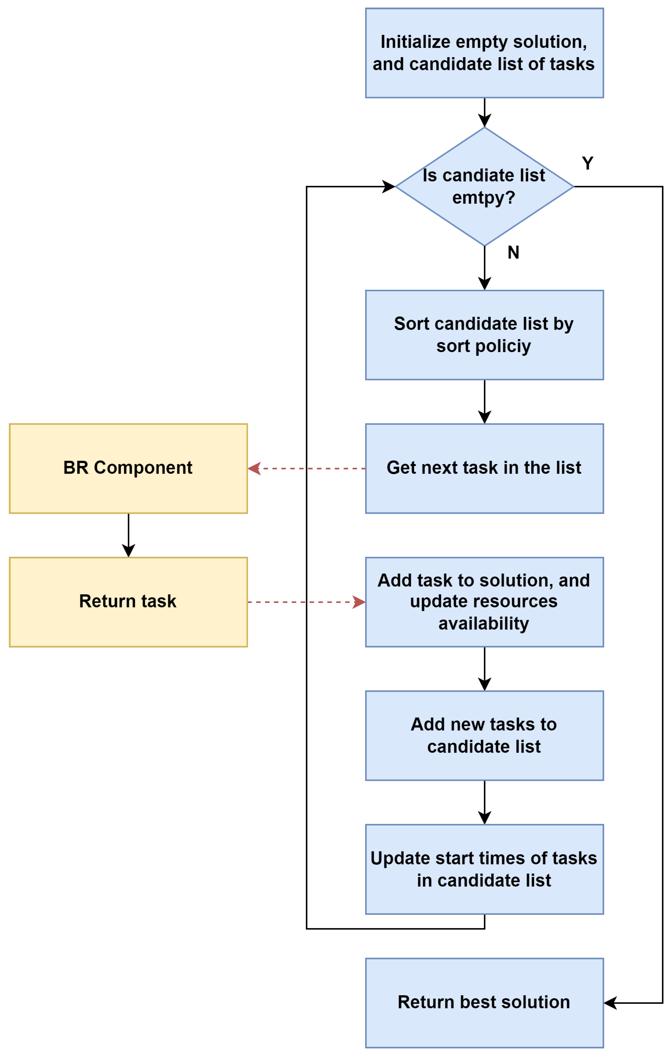
The novel DEH starts generating a new solution which includes an empty list of tasks. In addition, a list of candidate tasks is initialized with tasks without predecessors, also referred to as start or root tasks. The tracking of resource units allocated to tasks is managed through a cache mechanism, whose availability times are initialized to zero for all resources. The cache facilitates fast access to and management of availability times associated with individual resource units. Next, the algorithm iterates until the list of candidate tasks is empty. At each iteration, the candidate list is sorted based on the sort policy passed as input. Next, the next task to be scheduled is selected from the list of candidate tasks. In the deterministic version of the DEH algorithm, the task with the optimal value for the selected sorting policy is chosen. However, this changes under the biased-randomized (non-deterministic) approach. Each candidate task has a probability of being selected. This probability is not evenly distributed, meaning tasks closer to the first element in the list are more likely to be chosen than the tasks further from the start. Individual probabilities are modeled by a skewed geometric probability distribution function which requires a probability coefficient called $\beta \in (0,1)$. This approach ensures that the same solution is not obtained repeatedly and allows for the discovery of solutions that outperform those obtained through purely greedy behavior. Thus, the next task is extracted from the list of candidates in a biased-randomized manner, which employs the generated $\beta$ parameter passed as input for the DEH algorithm. The chosen task is then added to the solution, and the algorithm updates the availability times of allocated resources. In other words, when a new task is scheduled in the solution, the resources cache updates the availability times of the units allocated to the scheduled task. Subsequently, the algorithm inserts the task successors whose predecessors have been scheduled in the list of candidate tasks to schedule next. This step ensures that the dependencies between tasks are maintained since a task can only be inserted in the solution if all its predecessors have finished. Finally, for each task remaining in the list of candidate tasks, the possible starting times are adjusted based on the updated availability times of resource units. This iterative process continues until all tasks are scheduled. Lastly, the solution makespan is computed as the finish time of the project finis dummy task, and the solution is returned from the procedure. Figure 3 depicts the main characteristics of our novel DEH procedure.

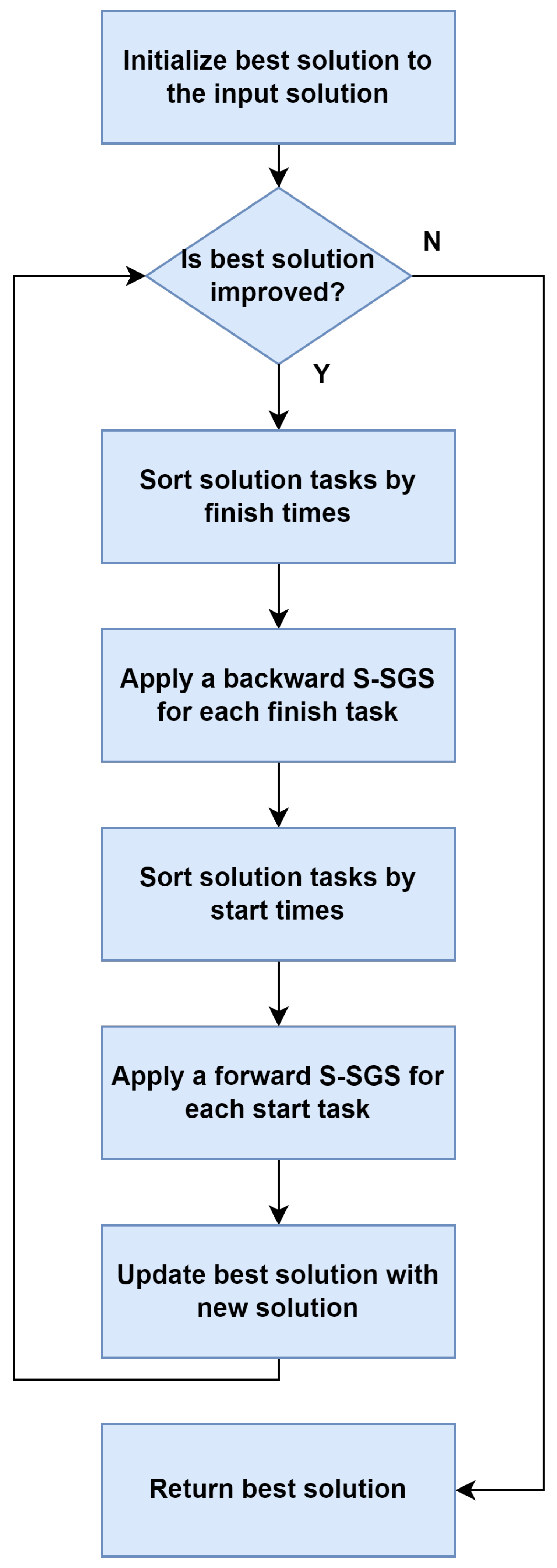
The extended FBI local search operator starts assigning a solution, which has been generated by the BR-DEH algorithm, as the best solution obtained so far. Next, the local search operator iteratively schedules the solution backward and forward until no further improvement occurs in the solution makespan. At each iteration, a backward S-SGS is applied to the best solution for each finished task (i.e., a task with no successors) and the tasks are shifted right to their latest feasible start times. Specifically, a task list is first created sorting the best solution tasks in decreasing order by their scheduled finish times. Next, the finished tasks of the solution are obtained and inserted one at a time in the last position of the task list. For each finished task, the backward sequence is built by scheduling each task i (following the task list order) as late as possible in the time window delimited by $[S_i,min(S_j^{\prime })]$, $\forall (i,j)\in A$, where $S_i$ refers to the start time of task i in the best solution, $S_j^{\prime }$ to the start time of task j in the partial backward sequence, and A to the set of precedence relations. Afterward, a forward S-SGS is also applied to the new solution obtained by the backward pass for each start task (i.e., a task with no predecessors) and the tasks are shifted left to their earliest start times. Specifically, a task list is first created sorting the new solution tasks in increasing order of their scheduled start times. Next, the start tasks of the solution are obtained and inserted one at a time in the first position of the list. For each start task, the forward sequence is built by scheduling each task i as early as possible (and following the task list order) in the time window delimited by $max(F_j^{\prime }),F_i$, $\forall (j,i)\in A$, where $F_i$ refers to the finish time of task i in the previous backward sequence, $F_j^{\prime }$ to the finish time of task j in the partial forward sequence, and A to the set of precedence relations. If the newly generated solution after the forward pass improves the best solution obtained so far, the best solution is updated and the improvement procedure schedules the best solution backward and forward again. Notice that in successive iterations, this local search operator never obtains a makespan greater than the best solution makespan, since the best solution makespan is passed to the backward pass as the project duration to start the schedule from. In addition, the generation of several backward and forward S-SGS ensures the exploration of more solution schedules. Thus, increasing the solution space and obtaining more solutions; some of them outperformed the ones obtained using the standard FBI local search operator. Once the solution does not improve, the best solution obtained so far is returned from the procedure. Figure 4 outlines the principal components of the extended FBI local search operator.

Lastly, the path relinking procedure is similar to the procedure of Ranjbar and Kianfar [44]. However, our path relinking procedure is applied to the most promising solutions generated by the multi-start process of the BR-DEH algorithm. The procedure starts by iterating each pair of solutions in the elite solutions list and identifying for each pair the initiating and guiding solutions. Our path relinking procedure assigns the solution with the lowest makespan to be the guiding solution, and the opposite solution to be the initiating solution. Next, new solutions are generated by exploring the trajectory that connects the initiating solution to the guiding solution. This is accomplished by selecting moves that introduce attributes contained in the guiding solution, and incorporating them in a newly generated solution initially originated in the initiating solution. Specifically, we start generating a new solution which will be a copy of the initiating solution. Next, the tasks in the new solution are iterated. At each iteration, a task in the new solution is compared with the task in the same position in the guiding solution. If the tasks are different, the two tasks in the new solution are swapped. Next, a feasibility check is performed, as the order of the tasks should be precedence feasible. Specifically, if a task is a predecessor of one of the following tasks in the solution, it swaps its positions to maintain precedence feasibility. If the newly generated solution, which is now precedence feasible, outperforms the best solution found so far, the best solution is updated with the new solution. Once every task in the new solution is iterated, the next pair of solutions is considered. Finally, once every pair of solutions has been considered, the best solution is returned from the procedure.

The computational complexity of the DEH algorithm was rigorously analyzed, revealing its practical efficiency and robustness. The initialization phase involves resetting task predecessors and resource availability times, which collectively operate in $O(T+R)$ time, where T and R represent the number of tasks and resources, respectively. During the main execution loop, tasks are selected, scheduled, and updated in constant time $O\left(1\right)$. Resource availability updates and the recalculation of task start times involve more complex operations bounded by $O(R·UlogU)$ and $O(C·R·U)$, where U denotes the maximum units of resources per task, and C is the realistic maximum size of the candidate list. Additionally, sorting the candidate list by the selected policy introduces a complexity of $O\left(C^2\right)$. We use an insertion sort algorithm as practically, the size of the candidate list is smaller, and thus more efficient than a more standard sorting algorithm. Given the iterative nature of the algorithm over all tasks, the cumulative complexity is $O(T·(T+R·UlogU+C^2))$. However, since C is significantly smaller than T in practical scenarios, the dominant term simplifies to $O\left(T^2\right)$, underscoring the algorithm’s efficiency in handling large-scale scheduling problems with a complexity comparable to other heuristic approaches. This analysis highlights the algorithm’s scalability and its suitability for real-world applications, where it consistently delivers reliable and robust performance.

5. Computational Experiments

This section presents a detailed analysis of the performance of the BR-DEH algorithm. The algorithm is implemented in Julia 1.9.3 [45]. All computational experiments are conducted on a Linux Mint machine with a multi-core processor Intel Xeon E5-2630 v4 with 32 GB of RAM. The BR-DEH algorithm is evaluated using the well-known benchmark problem test set Project Scheduling Problem Library (PSPLIB) [46]. PSPLIB was generated by the project generator ProGen [47], which contains four sets, namely, $j30$, $j60$, $j90$, and $j120$, including 30, 60, 90, and 120 tasks, respectively. The sets $j30$, $j60$, and $j90$ include a total of 480 instances, whereas set $j120$ includes a total of 600 instances. The four sets are designed with network complexity, resource factor, and resource strength parameters. Additional details are described by Kolisch et al. [48]. The $j30$, $j60$, and $j120$ sets are used as benchmarks for evaluating the performance of the proposed BR-DEH algorithm. These sets are used as they facilitate comparisons with established classic algorithms found in existing literature. Following a standard practice in this field [49], the number of iterations is used as the stopping criterion. In this case, the numbers of iterations are defined as 1000, 5000, and 50,000. Each instance is executed 32 times with different seeds for the random number generator, and the best, and average results are reported. In addition, the FBI local search operator executes only one improvement iteration to sustain the algorithm’s performance and efficiency constraints. This notion is supported by the findings of Tormos and Lova [40], which analyzed the number of FBI passes, revealing a significant discovery regarding the iterative improvement process. Notably, regardless of the number of iterations executed, the most substantial improvement was consistently observed in the initial iteration.

The adaptive mechanism involves two stages: the biased-randomization parameter and the sorting policy selection. The biased-randomization process begins with a parameter $\beta$ set to an initial value of $0.5$. At each iteration of the BR-DEH algorithm, a new value of the $\beta$ parameter is randomly generated, denoted as ${\beta }^{\prime }$, which is used as the biased-randomization parameter to produce a new solution. As illustrated in Figure 5, to generate ${\beta }^{\prime }$ a triangular distribution function with a lower limit set to 0, upper limit set to 1, and the $\beta$ parameter serving as the mode is employed. If the newly generated solution obtains a lower makespan compared to the best solution obtained thus far, the $\beta$ parameter is set to the new ${\beta }^{\prime }$ value. Subsequently, the new ${\beta }^{\prime }$ value will be used as the mode for the subsequent iterations’ triangular distribution. Analyzing the behavior of the $\beta$ parameter, in the initial iterations of the algorithm, it undergoes oscillation which explores a range of different values. However, over successive iterations, this process tends to stabilize, ultimately converging towards an optimal $\beta$ that consistently generates high-quality solutions. This adaptive self-tuning process constitutes a robust approach, customizing the biased-randomization parameter specific to each instance. This method diverges from the conventional approach of defining a fixed interval for the $\beta$ parameter, providing a more efficient means to search for optimal solutions across various benchmark instances.

The sorting policy process, similar to the biased-randomization mechanism, starts with an initial sorting policy chosen from the list of policies. This sorting policy, assigned to be the best sorting policy found so far, is used to generate a feasible initial solution for the BR-DEH algorithm. At each iteration, a random sorting policy is selected using the following mechanism: with a $20\%$ probability, the algorithm either selects the current best sorting policy or randomly chooses one from the list of available policies. If the new solution generated with the chosen sorting policy surpasses the best solution found so far, the algorithm updates the best sorting policy accordingly. This continuous process enables the BR-DEH algorithm to dynamically oscillate between known effective sorting strategies and exploration of alternative policies, facilitating a constant evolution in the selection of the best sorting policy based on the observed performance of solutions across iterations. This adaptive mechanism aims to converge towards a sorting policy that significantly enhances the algorithm’s capability to obtain high-quality solutions. Sorting policies can be classified as follows: (i) policies that use network characteristics, (ii) policies that use time information, (iii) policies that use resource parameters, and (iv) policies that use a combination of the previous three rules [50].

Table 1. Sorting policies for selecting candidate tasks.

Sort Policy	Description	Formula
SAD	The task that has the minimum task duration is picked.	min $d_j$
MIS	The task that has the maximum number of successors is picked.	max $F_j$
MTS	The task that has the maximum number of total successors is picked.	max $F_j^{*}$
HRPW	The task that has the first highest rank positional weight is picked. This is calculated as the duration of the task plus the sum of the durations of all immediate successors.	max $(d_j+{\sum }_{i\in F_j}{d}_i)$
HRPW*	The task that has the second highest rank positional weight is picked. This is calculated as the duration of the task plus the sum of the durations of all total successors.	max $(d_j+{\sum }_{i\in F_j^{*}}{d}_i)$
EFT	The task with the earliest finish time is picked. This is calculated using the initial CPM earliest finish time.	min $EF{T}_j$
EFTD	The task with the earliest dynamic finish time is picked. This is calculated by updating the CPM values in each step of the resource allocation process.	min $EFT{D}_j$
LST	The task with the earliest late start time is picked. This is calculated using the initial CPM’s latest start time.	min $LS{T}_j$
LFT	The task with the earliest late finish time is picked. This is calculated using the initial CPM’s latest finish time.	min $LF{T}_j$
STFS	The task with the smallest static total float is picked. This is calculated as the difference between the latest start time and the earliest start time.	min $LS{T}_j-ES{T}_j$
STFD	The task with the smallest dynamic total float is picked. This is calculated as the difference between the latest start time and the dynamic earliest start time updated at each step of the resource allocation process.	min $LS{T}_j-EST{D}_j$
HRD	The task with the highest resource demand is picked. This is calculated as the product of the duration of the task with all resource units of each resource type used to perform the task.	max $(d_j\times {\sum }_{r=1}^m{u}_{jr})$
HWRU	The task with the highest weighted resource utilization and number of successor tasks is picked. This is computed as a linear combination of the immediate successors of the task and the percentage of resource units of each resource type used.	max $\left[\right(\omega \times |F_j\left|\right)+(1+\omega )\times {\sum }_{r=1}^m\left(\frac{u_{jr}}{a_r}\right)]$

presents 13 sorting policies collected by Klein [51]. The first column represents the sorting policy abbreviations, the second column presents a brief description, and the third column shows the formula to compute each sorting policy. The BR-DEH algorithm sorts tasks in increasing order based on their possible start times. In cases where tasks share identical start times, it employs one of the policies presented below to break ties.

These sorting policies control the order of tasks based on their start times and resource requirements, allowing for the prioritization of tasks during the solution construction process. The BR-DEH algorithm uses a range of sorting strategies, where each sorting policy addresses specific aspects of project scheduling and resource allocation. This contributes to the algorithm’s adaptability and capability to explore and exploit the search space effectively. Thus, the combination of sorting policies within the BR-DEH algorithm enables custom and dynamic decision-making, facilitating the search for high-quality solutions in various optimization scenarios.

6. Analysis of Results

Table 2. Best results of the proposed BR-DEH algorithm.

Instance Set		Number of Iterations
		1000	5000	50,000
j30	BEST GAP (%)	0.02	0.01	0.00
	BEST CPU (s)	0.03	0.15	1.48
j60	BEST GAP (%)	11.10	10.91	10.70
	BEST CPU (s)	0.07	0.34	3.21
j120	BEST GAP (%)	33.34	32.55	32.22
	BEST CPU (s)	0.32	1.27	10.34

displays the best results obtained by the proposed BR-DEH algorithm. For the set $j30$, the results of the algorithm are compared with the optimal makespan of all instances provided by the PSPLIB. However, for the sets $j60$, and $j120$, the obtained results are compared with the lower and upper bounds as the optimal makespan is not known. The lower bounds are calculated by the critical path method (CPM) of the resource-unconstrained problem, whereas the upper bounds are the best solutions computed by various metaheuristics published in the literature. The first column reports the problem set, while the remaining columns report the best results obtained by the BR-DEH algorithm for different numbers of iterations. For each problem set, we report the average percentage gap obtained with respect to the optimal makespan or lower bound, and the average computational time used to obtain the best-found solution. The obtained results show that, as with any other algorithm solving NP-hard problems, the performance is influenced by the number of tasks in the project, as the average computational time increases as the size of the problem increases. Specifically, set $j30$ comprises the simplest instances, as the BR-DEH algorithm consistently finds the optimal solution for different numbers of iterations. On the other hand, sets $j60$, and $j120$ consist of instances that pose greater difficulty in achieving high-quality solutions. However, the BR-DEH is able to generate high-quality solutions in just a few seconds of computational time, even for the largest and most difficult set.

Observe that the BR-DEH algorithm achieves, in just 50,000 iterations, percentage gaps of $0.00\%$, $10.70\%$, and $32.22\%$ for the optimal values or lower bounds for the sets $j30$, $j60$, and $j120$, respectively. Specifically, it consistently delivers highly competitive solutions for problems with a smaller number of tasks. Moreover, the BR-DEH approach delivers high-quality solutions even for instances with a higher number of tasks. Notice that the average CPU times demonstrate the algorithm’s computational efficiency in solving these instances. For average CPU times of 1.48 s, 3.21 s, and 10.34 s, for sets $j30$, $j60$, and $j120$, respectively. Thus, the BR-DEH algorithm shows remarkable effectiveness in delivering solutions within low computational times. These results underscore the scalability of the algorithm, as it obtains high-quality solutions in $10 \mathrm{s}$ for the largest instance set.

Table 3. Average results of the proposed BR-DEH algorithm.

Instance Set		Number of Iterations
		1000	5000	50,000
j30	AVG. GAP (%)	0.13	0.04	0.02
	STD. DEV (%)	0.51	0.26	0.19
j60	AVG. GAP (%)	11.63	11.23	11.08
	STD. DEV (%)	23.20	22.69	22.41
j120	AVG. GAP (%)	34.58	33.65	33.28
	STD. DEV (%)	46.31	45.64	45.32

displays the average results obtained by the proposed BR-DEH algorithm. The first column reports the problem set, while the remaining columns report the average results obtained by the BR-DEH algorithm for different numbers of iterations. For each problem set, we report the average percentage gap and standard deviation obtained with respect to the optimal makespan or lower bound. The obtained results show that the average results are not that far from the best results reported in the previous paragraphs. In other words, the results given by the different executions are really close to the best result, which shows that the algorithm is reliable and robust. The reliability and robustness of the BR-DEH approach are further underscored by its consistent performance, rapidly converging to the optimal makespan in repeated trials. This consistent performance across multiple runs demonstrates the algorithm’s effectiveness in providing high-quality solutions with minimal deviation, ensuring dependable outcomes in practical applications.

Focusing on a particular instance, we conduct a convergence analysis for a randomly selected instance from the $j120$ set. Figure 6 shows the convergence plot for the $j12014\_3.sm$ instance. Observe that, the convergence plot demonstrates the efficiency of the BR-DEH approach in rapidly reaching optimal solutions. Specifically, the initial makespan starts at 90 and swiftly declines to 88, the optimal value, within just a few iterations. The fast convergence can be attributed to the novel DEH approach, which generates good-quality solutions to be improved by the extended FBI operator. This indicates that the BR-DEH method effectively narrows the search space and finds optimal or near-optimal solutions quickly, minimizing the time and computational resources required to achieve the desired solutions.

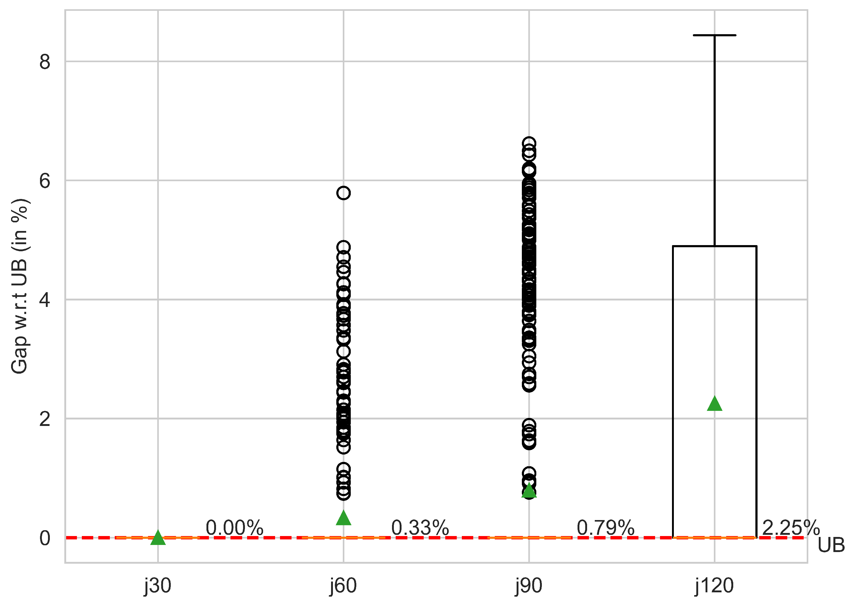
Figure 7 and Figure 8 depict two box plots that summarize the computational results with respect to the upper bound and lower bound values, respectively. The horizontal axis represents the different instance sets, while the vertical axis represents the computed gap between the best-found solutions by the BR-DEH algorithm and the upper bound and lower bound values. Green triangles represent average values, while circles represent outliers. Looking at the first box plot, it can be noted that for the $j30$ set we obtain the best-known solution for all the instances. As for the $j60$, and $j90$ sets we obtain the best-known solution for most of the instances, but there are some instances for which the optimal upper bound value is not reached. This can be seen with the outlier points that fall outside the whiskers of the box plot. Finally, the obtained gaps for the $j120$ are more spread out, meaning that we obtain solutions near the upper bound values but not always the best-known solution.

In the interest of thoroughness, a more comprehensive comparison of the results of the BR-DEH algorithm is conducted. This is conducted using the CPM lower bound values, as the computed percentage gaps with respect to the upper bounds will not be relevant once new best solutions are obtained.

Table 4. Average percentage deviations from the optimal makespan for set $j30$.

Algorithm	Reference	Number of Iterations
		1000	5000	50,000
BR-DEH	This study	0.02	0.01	0.00
GA-self-adapting	Hartmann [52]	0.38	0.22	0.08
GA, TS-path relinking	Kochetov and Stolyar [42]	0.10	0.04	0.00
SS-EM	Debels et al. [53]	0.27	0.11	0.01
DBGA	Debels and Vanhoucke [54]	0.12	0.04	0.02
Hybrid GA	Valls et al. [55]	0.27	0.06	0.02
ESS-FBI-path relinking	Mahdi Mobini et al. [43]	0.05	0.02	0.01
GAPS	Mendes et al. [56]	0.06	0.02	0.01
ACOSS	Chen et al. [57]	0.14	0.06	0.01
JPSO	Chen [58]	0.29	0.14	0.04
Neurogenetic-FBI	Agarwal et al. [59]	0.13	0.10	—
Art. Imm. Alg	Mobini et al. [60]	0.05	0.03	0.00
BA-FBI	Ziarati et al. [61]	0.42	0.09	0.04
GA-FBI-Random key	Gonçalves et al. [62]	0.32	0.02	0.01
SFLA	Wang and Fang [63]	0.36	0.21	0.18
PSO-FBI-path relinking	Nasiri [64]	0.30	0.10	0.01
HGA	Lim et al. [26]	0.21	0.07	0.01
PSOHH	Koulinas et al. [65]	0.26	0.04	0.01
GA-Part	Zamani [66]	0.17	0.07	0.01
COAs	Elsayed et al. [67]	0.04	0.00	0.00
GA-FBI	Liu et al. [68]	0.24	0.06	0.01

,

Table 5. Average percentage deviations from the lower bound for set $j60$.

Algorithm	Reference	Number of Iterations
		1000	5000	50,000
BR-DEH	This study	11.10	10.91	10.70
GA-self-adapting	Hartmann [52]	12.21	11.27	10.74
GA, TS-path relinking	Kochetov and Stolyar [42]	11.71	11.17	10.74
SS-EM	Debels et al. [53]	11.73	11.10	10.71
DBGA	Debels and Vanhoucke [54]	11.31	10.95	10.68
Hybrid GA	Valls et al. [55]	11.56	11.10	10.73
ESS-FBI-path relinking	Mahdi Mobini et al. [43]	11.12	10.74	10.57
GAPS	Mendes et al. [56]	11.72	11.04	10.67
ACOSS	Chen et al. [57]	11.75	10.98	10.67
JPSO	Chen [58]	12.03	11.43	11.00
Neurogenetic-FBI	Agarwal et al. [59]	11.51	11.29	—
Art. Imm. Alg	Mobini et al. [60]	11.17	10.80	10.55
BA-FBI	Ziarati et al. [61]	12.55	12.04	11.16
GA-FBI-Random key	Gonçalves et al. [62]	—	11.56	10.57
SFLA	Wang and Fang [63]	11.44	10.87	10.66
PSO-FBI-path relinking	Nasiri [64]	12.02	11.33	11.79
HGA	Lim et al. [26]	11.73	11.14	10.63
PSOHH	Koulinas et al. [65]	11.74	11.13	10.68
GA-Part	Zamani [66]	11.61	11.08	10.71
COAs	Elsayed et al. [67]	11.13	10.77	10.58
GA-FBI	Liu et al. [68]	11.74	11.15	10.66

and

Table 6. Average percentage deviations from the lower bound for set $j120$.

Algorithm	Reference	Number of Iterations
		1000	5000	50,000
BR-DEH	This study	33.34	32.55	32.22
GA-self-adapting	Hartmann [52]	37.19	35.39	33.21
GA, TS-path relinking	Kochetov and Stolyar [42]	34.74	33.36	32.06
SS-EM	Debels et al. [53]	35.22	33.10	31.57
DBGA	Debels and Vanhoucke [54]	33.55	32.18	30.69
Hybrid GA	Valls et al. [55]	34.07	32.54	31.24
ESS-FBI-path relinking	Mahdi Mobini et al. [43]	34.51	32.61	31.37
GAPS	Mendes et al. [56]	35.87	33.03	31.44
ACOSS	Chen et al. [57]	35.19	32.48	30.56
JPSO	Chen [58]	35.71	33.88	32.89
Neurogenetic-FBI	Agarwal et al. [59]	34.65	34.15	—
Art. Imm. Alg	Mobini et al. [60]	34.01	32.57	31.48
BA-FBI	Ziarati et al. [61]	37.72	36.76	34.55
GA-FBI-Random key	Gonçalves et al. [62]	—	35.94	32.76
SFLA	Wang and Fang [63]	34.83	33.20	31.11
PSO-FBI-path relinking	Nasiri [64]	36.77	35.16	32.89
HGA	Lim et al. [26]	34.95	32.75	30.66
PSOHH	Koulinas et al. [65]	35.20	32.59	31.23
GA-Part	Zamani [66]	34.59	33.36	31.81
COAs	Elsayed et al. [67]	34.04	32.90	31.22
GA-FBI	Liu et al. [68]	34.88	33.00	31.15

present a comparison of the BR-DEH approach with the results obtained by some state-of-the-art algorithms for solving the RCPSP found in the literature. The selection of these algorithms was based on their availability of reported results for different numbers of iterations. The results of the reported algorithms can be obtained from the original studies. The $j30$, $j60$, and $j120$ sets have been displayed as they facilitate comparisons with the established state-of-the-art algorithms.

Observe that the BR-DEH algorithm reports average results competitively when compared with the established state-of-the-art algorithms found in the literature. Specifically, for the $j30$ set, the proposed BR-DEH algorithm ranks first, second and first in 1000, 5000, and 50,000 number of iterations, respectively. As for the $j60$ set, the proposed BR-DEH algorithm ranks first, third, and 12th for 1000, 5000, and 50,000 number of iterations, respectively. Lastly, for the $j120$ set, the BR-DEH algorithm ranks first, fourth, and 15th for 1000, 5000, and 50,000 number of iterations, respectively. Observe that, the BR-DEH consistently achieves near-optimal solutions, showcasing its effectiveness across various problem instances. The difference in performance as the number of iterations increases can be attributed to the algorithm designs, as the other state-of-the-art algorithms are evolutive algorithms that explore the solution space with multiple individuals, while the BR-DEH algorithm generates only one solution per iteration. In other words, this disparity comes from the exploration of the solution space at every iteration, since the BR-DEH algorithm generates one solution while the other algorithms generate multiple solutions per iteration. However, evolutive algorithms exhibit high computational times, especially when dealing with complex problems or large solution spaces. This is due to their iterative nature and reliance on population-based exploration, which often involves evaluating a large number of candidate solutions across multiple generations. In contrast, the BR-DEH algorithm stands out, achieving high-quality solutions for a lower number of iterations with an average computational time of 5.01 s. Thus, when comparing the lower bound values with the best solutions computed by other state-of-the-art algorithms published in the literature, the BR-DEH approach demonstrates a remarkable performance in terms of both solution quality and computational time.

In essence, the computational results highlight the strengths of the BR-DEH algorithm. First, the BR-DEH algorithm has an effective and relatively straightforward implementation, striking a favorable balance between computational performance and simplicity. This is contrasted with the often complex and intricate operators used in evolutionary methods. Next, an adaptive mechanism to tune the algorithm parameters is introduced, which avoids the necessity of the expensive prior analysis incurred in other state-of-the-art algorithms. Lastly, the out-solving method generates near-optimal solutions for a lower number of tasks, and high-quality solutions for a higher number of tasks in just a few seconds of computational time. This capability proves invaluable in industries where real-time solutions are needed for successful operations at the expense of solution quality.

7. Conclusions and Future Work

In this study, a novel agile BR-DEH algorithm is introduced to tackle the RCPSP. The methodology integrates a discrete-event heuristic with biased-randomization, combining speed and efficiency to produce high-quality solutions within short computational times. Additionally, an adaptive mechanism to fine-tune the algorithm’s parameters is proposed, contributing to its robustness and effectiveness across various problem instances. The evaluation of the BR-DEH algorithm was conducted using benchmark instances derived from the PSPLIB, offering a comparative analysis against state-of-the-art metaheuristics, which typically require higher computational times to provide similar results. The computational results highlight the algorithm’s capability, demonstrating competitive performance even with a limited computing time of just a few seconds of execution.

For the $j30$ set, the algorithm consistently produced solutions within a $0.00\%$ deviation from the optimal makespan, showcasing its ability to achieve optimal solutions for simpler instances. When faced with more complex scenarios in the $j60$ and $j120$ sets, the algorithm exhibited percentage gaps of $10.70\%$, and $32.22\%$ with respect to the lower bounds, demonstrating its efficiency in delivering high-quality solutions in just a few seconds for more challenging problem instances. These findings emphasize the algorithm’s robustness and competitive edge, achieving remarkable performance metrics within notably low computational times (1.48 s, 3.21 s, and 10.34 s for $j30$, $j60$, and $j120$, respectively).

Several potential directions for future research to expand upon the current work are outlined next: (i) consider the inclusion of uncertainty in task duration or resource units, which could involve extending the DEH algorithm into a simulation-optimization framework such as simheuristics [69]; (ii) extend the applicability and efficiency of the proposed BR-DEH algorithm to complex construction project scheduling problems, such as the RCPSP with generalized precedence relations; (iii) use more sophisticated high-performance computing techniques to obtain near-optimal solutions in real-time that react to changes in the initial project planning, such as the possible variability of the makespan when faced with disruptions in resource units or when faced with the inclusion or cancellation of tasks.