A Legendre Spectral-Element Method to Incorporate Topography for 2.5D Direct-Current-Resistivity Forward Modeling

Abstract

An effective and accurate solver for the direct-current-resistivity forward-modeling problem has become a cutting-edge research topic. However, computational limitations arise due to the substantial amount of data involved, hindering the widespread use of three-dimensional forward modeling, which is otherwise considered the most effective approach for identifying geo-electrical anomalies. An efficient compromise, or potentially an alternative, is found in two-and-a-half-dimensional (2.5D) modeling, which employs a three-dimensional current source within a two-dimensional subsurface medium. Consequently, a Legendre spectral-element algorithm is developed specifically for 2.5D direct-current-resistivity forward modeling, taking into account the presence of topography. This numerical algorithm can combine the complex geometric flexibility of the finite-element method with the high precision of the spectral method. To solve the wavenumber-domain electrical potential variational problem, which is converted into the two-dimensional Helmholtz equation with mixed boundary conditions, the Gauss–Lobatto–Legendre (GLL) quadrature is employed in all discrete quadrilateral spectral elements, ensuring identical Legendre polynomial interpolation and quadrature points. The Legendre spectral-element method is applied to solve a two-dimensional Helmholtz equation and a resistivity half-space model. Numerical experiments demonstrate that the proposed approach yields highly accurate numerical results, even with a coarse mesh. Additionally, the Legendre spectral-element algorithm is employed to simulate the apparent resistivity distortions caused by surface topographical variations in the direct-current resistivity Wenner-alpha array. These numerical results affirm the substantial impact of topographical variations on the apparent resistivity data obtained in the field. Consequently, when interpreting field data, it is crucial to consider topographic effects to the extent they can be simulated. Moreover, our numerical method can be extended and implemented for a more accurate computation of three-dimensional direct-current-resistivity forward modeling.

1. Introduction

The direct-current-resistivity exploration method is a powerful geophysical tool used to non-invasively investigate subsurface properties of the Earth. This method entails measuring the electrical resistivity of various materials and structures beneath the surface by transmitting a direct current through the ground and assessing the resulting potential differences. Due to their environmentally friendly nature and cost-effectiveness, direct-current measurements have found extensive application in diverse fields, including engineering studies [1,2,3,4], hydro-geological work [5,6,7], mineral resource exploration [8,9], and humanitarian geophysics [10]. In these geophysical explorations, the topography is typically non-flat, and the presence of the terrain will lead to false anomalies in apparent resistivity [11]. Hence, incorporating these topographic effects into the numerical solutions of the direct-current resistivity forward problem is essential for generating accurate models.

Numerical modeling approaches, such as the finite-difference method (FDM) [12,13,14,15] and finite-element method (FEM) [16,17,18], have been applied for high-dimensional direct-current-resistivity forward modeling and inversion. The FDM utilizes difference operators to approximate the first or second partial derivatives in the partial differential equation (PDE), but its effectiveness is limited to a relatively flat topography. On the other hand, the FEM converts the PDE into an integral equation using a Galerkin scheme or variational principle, and subsequently performs numerical integration. Previous studies on incorporating topography into two-dimensional and three-dimensional direct-current-resistivity computational modeling have primarily focused on the FEM.

The computational modeling partial differential equation (PDE) has demonstrated that the spectral-element method possesses more appealing characteristics compared to the traditional FDM and FEM. As a high-order finite-element approach, the spectral-element method can combine the complex geometric flexibility of the FEM with the high accuracy of the spectral method [19,20]. The finite-element method enables the simulation of complex real-world information, including topography and bathymetry, while enhancing the flexibility of discretization domains in 2D and 3D conductivity models. In contrast, the spectral method, as an innovative numerical technique, can achieve accurate solutions for geophysical ordinary differential equations or partial differential equations [21]. Owing to its high numerical accuracy and geometric flexibility, the spectral-element method has found widespread application in geophysical forward-modeling problems [22,23,24,25,26]. Therefore, the spectral-element scheme can be adapted for direct-current-resistivity modeling involving topography, yielding high-precision numerical solutions.

In this study, a Legendre spectral-element algorithm is developed for computational modeling of a 2.5D direct-current-resistivity problem incorporating topography. In order to test numerical accuracy, we compare the spectral-element approximate results with the corresponding analytical solutions. Furthermore, numerical modeling examples are provided to validate the efficacy of the spectral-element technique and demonstrate the significance of topographic effects.

The remainder of this paper is organized as follows. Section 2 introduces the Helmholtz-type equation for the Fourier-domain electrical potential within the framework of 2.5D direct-current resistivity. Section 3 presents a high-performance implementation of the spectral-element algorithm with the Gauss–Lobatto–Legendre interpolation technique for the 2.5D direct-current-resistivity forward problem. Section 4 utilizes numerical experiments to verify the accuracy and efficiency of the proposed forward algorithm. Section 5 illustrates the topographic effects on apparent resistivity. Finally, the main conclusions are summarized in Section 6.

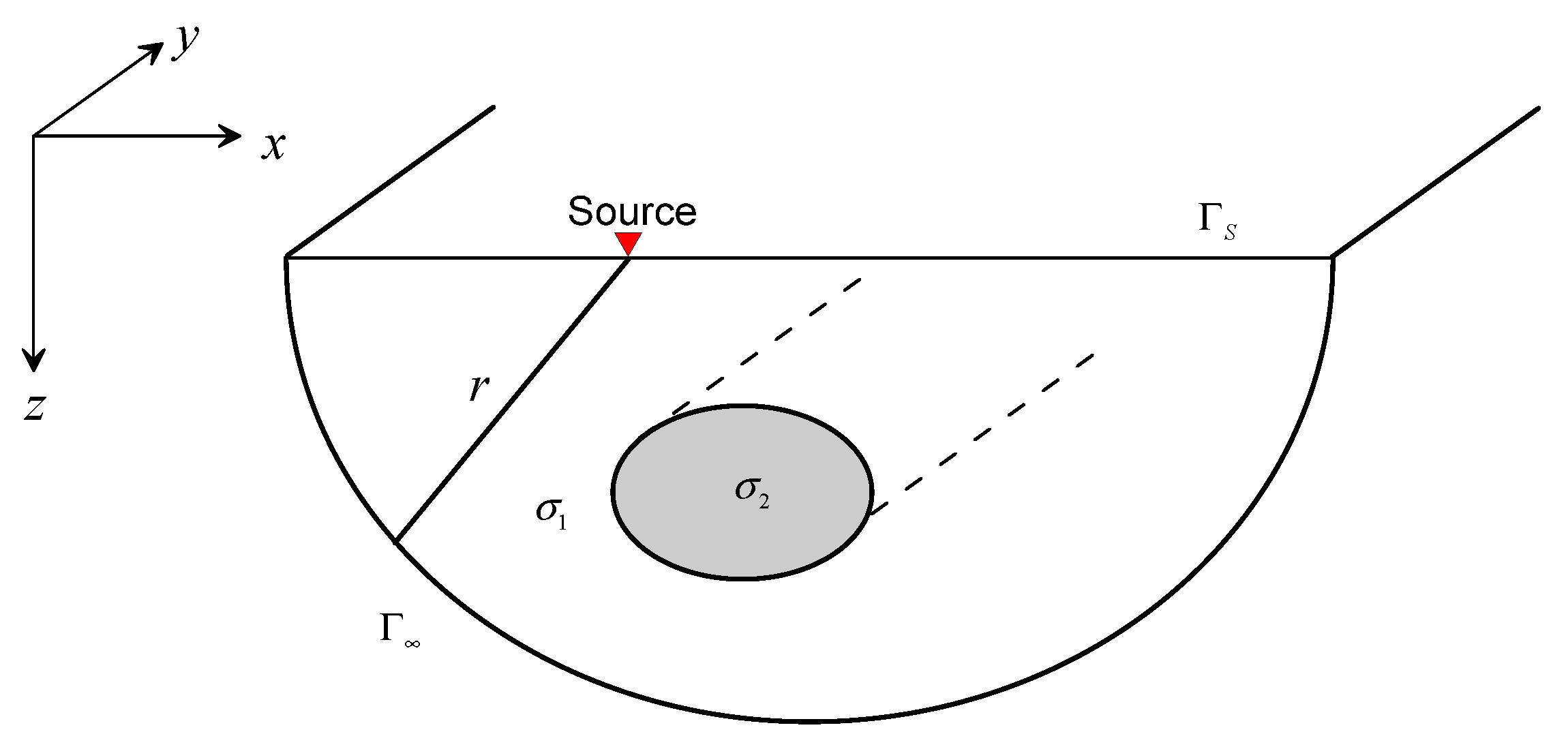
2. Mathematical Problem

Considering the Cartesian coordinate system $\left(x,y,z\right)$, a current point-source I is placed at a source point $\left(x_S,y_S,z_S\right)$ in a three-dimensional geo-electrical model. Then, the corresponding three-dimensional electrical potential $u\left(x,y,z\right)$ in the space domain can be governed by a Poisson-type equation [27,28]:

$$\begin{array}{l}\frac{\partial }{\partial x}\left[\sigma \left(x,y,z\right)\frac{\partial u}{\partial x}\right]+\frac{\partial }{\partial y}\left[\sigma \left(x,y,z\right)\frac{\partial u}{\partial y}\right]+\frac{\partial }{\partial z}\left[\sigma \left(x,y,z\right)\frac{\partial u}{\partial z}\right]\\ \hspace{1em}=-2I\delta \left(x-x_S\right)\delta \left(y-y_S\right)\delta \left(z-z_S\right)\end{array}$$

(1)

where $\sigma \left(x,y,z\right)$ is the three-dimensional conductivity, $\sigma \left(x,y,z\right)$, of the subsurface medium ($\mathrm{S}/\mathrm{m}$), which is the inverse of resistivity, $\rho \left(x,y,z\right)$ ($\Omega \cdot \mathrm{m}$), and $\delta$ is the Dirac distribution function.

At the interface ${\Gamma }_S$ between air and earth, the space-domain electrical potentials satisfy the Neumann-type boundary conditions:

$${\left.\frac{\partial u}{\partial n}\right|}_{{\Gamma }_S}=0$$

(2)

On the external truncated or distant boundary, ${\Gamma }_{\infty }$, the Robin-type conditions can be expressed as follows:

$${\left.\left[\frac{\partial u}{\partial n}+\frac{\cos \left(r,n\right)}{r}u\right]\right|}_{{\Gamma }_{\infty }}=0$$

(3)

where r represents the radial distance from the current point-source point to the boundary, and n denotes the outward normal direction on the distant boundary, ${\Gamma }_{\infty }$. This mixed condition is derived by eliminating the explicit dependence of the electrical potential on the conductivity.

Assuming no variation in the conductivity or resistivity data in the y (strike) direction, as depicted in Figure 1, Equation (1) can be rewritten as follows:

$$\begin{array}{l}\frac{\partial }{\partial x}\left[\sigma \left(x,z\right)\frac{\partial u\left(x,y,z\right)}{\partial x}\right]+\frac{\partial }{\partial y}\left[\sigma \left(x,z\right)\frac{\partial u\left(x,y,z\right)}{\partial y}\right]+\frac{\partial }{\partial z}\left[\sigma \left(x,z\right)\frac{\partial u\left(x,y,z\right)}{\partial z}\right]\\ \hspace{1em}=-2I\delta \left(x-x_S\right)\delta \left(y-y_S\right)\delta \left(z-z_S\right)\end{array}$$

(4)

In Equation (4), the electrical potential and the source term are three-dimensional functions of x, y, and z, while the conductivity parameter is a two-dimensional function of x and z. For the convenience of computational modeling, it is advantageous to solve this equation in Fourier space $\left(x,\lambda ,z\right)$ by transforming y into the wavenumber domain. The Fourier cosine transform can be used and is defined as follows:

$$U\left(x,\lambda ,z\right)={\displaystyle {\int }_0^{+\infty }u\left(x,y,z\right)\cos \left(\lambda y\right)\mathrm{d}y}$$

(5)

where $\lambda$ represents the wavenumber, and $U\left(x,\lambda ,z\right)$ represents the electrical potential in the Fourier domain or wavenumber domain.

By applying the forward Fourier cosine transform, the first term in Equation (4) is simplified as

$$\begin{array}{l}{\displaystyle {\int }_0^{+\infty }\frac{\partial }{\partial x}\left[\sigma \left(x,z\right)\frac{\partial u\left(x,y,z\right)}{\partial x}\right]\cos \left(\lambda y\right)\mathrm{d}y}=\frac{\partial }{\partial x}\left[\sigma \left(x,z\right)\frac{\partial }{\partial x}{\displaystyle {\int }_0^{\infty }u\left(x,y,z\right)\cos \left(\lambda y\right)\mathrm{d}y}\right]\\ =\frac{\partial }{\partial x}\left[\sigma \left(x,z\right)\frac{\partial U\left(x,\lambda ,z\right)}{\partial x}\right]\end{array}$$

(6)

The second term in Equation (4) can be expressed as

$$\begin{array}{l}{\displaystyle {\int }_0^{+\infty }\frac{\partial }{\partial y}\left[\sigma \left(x,z\right)\frac{\partial u\left(x,y,z\right)}{\partial y}\right]\cos \left(\lambda y\right)\mathrm{d}y}=\sigma \left(x,z\right){\displaystyle {\int }_0^{+\infty }\cos \left(\lambda y\right)\mathrm{d}}\frac{{\partial }^{2}u\left(x,y,z\right)}{\partial y^2}\\ =-{\lambda }^2\sigma \left(x,z\right)U\left(x,\lambda ,z\right)\end{array}$$

(7)

The third term in Equation (4) can be expressed as

$$\begin{array}{l}{\displaystyle {\int }_0^{+\infty }\frac{\partial }{\partial z}\left[\sigma \left(x,z\right)\frac{\partial u\left(x,y,z\right)}{\partial z}\right]\cos \left(\lambda y\right)\mathrm{d}y}=\frac{\partial }{\partial z}\left[\sigma \left(x,z\right)\frac{\partial }{\partial z}{\displaystyle {\int }_0^{\infty }u\left(x,y,z\right)\cos \left(\lambda y\right)\mathrm{d}y}\right]\\ =\frac{\partial }{\partial z}\left[\sigma \left(x,z\right)\frac{\partial U\left(x,\lambda ,z\right)}{\partial z}\right]\end{array}$$

(8)

The right term in Equation (4) can be expressed as

$$-{\displaystyle {\int }_{-\infty }^{+\infty }2I\delta \left(x-x_S\right)\delta \left(y\right)\delta \left(z-z_S\right)\cos \left(\lambda y\right)\mathrm{d}y}=-I\delta \left(x-x_S\right)\delta \left(z-z_S\right)$$

(9)

Using the forward Fourier cosine transform, the Neumann-type boundary condition of Equation (2) can be rewritten as

$$\begin{array}{l}{\displaystyle {\int }_{-\infty }^{+\infty }{\left.\frac{\partial u}{\partial n}\right|}_{{\Gamma }_S}\cos \left(\lambda y\right)\mathrm{d}y}={\left.\frac{\partial u}{\partial n}{\displaystyle {\int }_{-\infty }^{\infty }u\left(x,y,z\right)\cos \left(\lambda y\right)\mathrm{d}y}\right|}_{{\Gamma }_S}\\ ={\left.\frac{\partial U}{\partial n}\right|}_{{\Gamma }_S}=0\end{array}$$

(10)

The Robin-type boundary condition of Equation (3) can be rewritten as

$${\displaystyle {\int }_{-\infty }^{+\infty }{\left.\left[\frac{\partial u}{\partial n}+\frac{\cos \left(r,n\right)}{r}u\right]\right|}_{{\Gamma }_{\infty }}\cos \left(\lambda y\right)\mathrm{d}y}={\left.\left[\frac{\partial U}{\partial n}+\lambda \frac{K_1\left(\lambda r\right)}{K_0\left(\lambda r\right)}\cos \left(r,n\right)U\right]\right|}_{{\Gamma }_{\infty }}=0$$

(11)

where $K_0$, $K_1$ represent the modified Bessel functions of the second kind of orders 0 and 1, respectively.

By combining Equations (6)–(11), the electrical potential $U\left(x,\lambda ,z\right)$ with a Helmholtz-type can be formulated as

$$\left.\begin{array}{l}\frac{\partial }{\partial x}\left(\sigma \frac{\partial U}{\partial x}\right)+\frac{\partial }{\partial z}\left(\sigma \frac{\partial U}{\partial z}\right)-{\lambda }^2\sigma U=-I\delta \left(x-x_S\right)\delta \left(z-z_S\right)\\ {\left.\frac{\partial U}{\partial n}\right|}_{{\Gamma }_S}=0\\ {\left.\left[\frac{\partial U}{\partial n}+\lambda \frac{K_1\left(\lambda r\right)}{K_0\left(\lambda r\right)}\cos \left(r,n\right)U\right]\right|}_{{\Gamma }_{\infty }}=0\end{array}\right\}$$

(12)

3. Legendre Spectral-Element Method

3.1. Variational Problem and Discretization

By utilizing the divergence theorem [29], Equation (12) can be reformulated as a variational problem in integral form:

$$\left.\begin{array}{l}F(U)={\displaystyle {\int }_{\Omega }\left[\frac{\sigma }{2}{\left(\nabla U\right)}^2+\frac{1}{2}{\lambda }^2\sigma U^2-I\delta \left(x-x_s\right)\delta \left(z-z_s\right)U\right]}\mathrm{d}x\mathrm{d}z\\ \hspace{1em}\hspace{1em}\hspace{1em}+\frac{1}{2}{\displaystyle {\int }_{{\Gamma }_{\infty }}\sigma \frac{\lambda K_1\left(\lambda r\right)\cos \left(r,n\right)}{K_0\left(\lambda r\right)}{U}^2}\mathrm{d}l\\ \\ \delta F(U)=0\end{array}\right\}$$

(13)

The whole computational domain for the 2.5D direct-current-resistivity forward problem is discretized into quadrilateral elements, as depicted in Figure 2. In numerical approximation, the wavenumber domain electrical potential can be expressed using the 2D interpolation basis function:

$$\mathit{U}={\displaystyle \sum _{i=1}^{N_r}{N}_i\left(\xi ,\eta \right)U_i}$$

(14)

where $N_i\left(\xi ,\eta \right)$ represents the interpolation basis functions, and $N_r$ denotes the number of basis functions per element.

The integration over the entire computational domain is decomposed into a sum of integrals over each discrete element, allowing Equation (13) to be expressed as the summation of integrals across individual elements

$$\begin{array}{l}F\left(U\right)={\displaystyle \sum {\displaystyle {\iint }_{{\mathsf{\Omega }}_e}\left[\frac{1}{2}\sigma {\left(\nabla U\right)}^2+\frac{1}{2}{\lambda }^2\sigma U^2-I\delta \left(x-x_s\right)\delta \left(z-z_s\right)U\right]}\mathrm{d}x\mathrm{d}z}\\ \hspace{1em}\hspace{1em}\hspace{1em}+{\displaystyle \sum {\displaystyle {\int }_{{\mathsf{\Gamma }}_e}\frac{1}{2}\sigma \frac{\lambda K_1\left(\lambda r\right)\cos \left(r,n\right)}{K_0\left(\lambda r\right)}{U}^2\mathrm{d}l}}\end{array}$$

(15)

where ${\Omega }_e$ represents the area of a specific element, e, ${\Gamma }_e$ signifies the surface on the truncated boundary, ${\Gamma }_{\infty }$, and $e=1,2,\cdots ,N_h$ with $N_h$ denoting the number of quadrilateral elements.

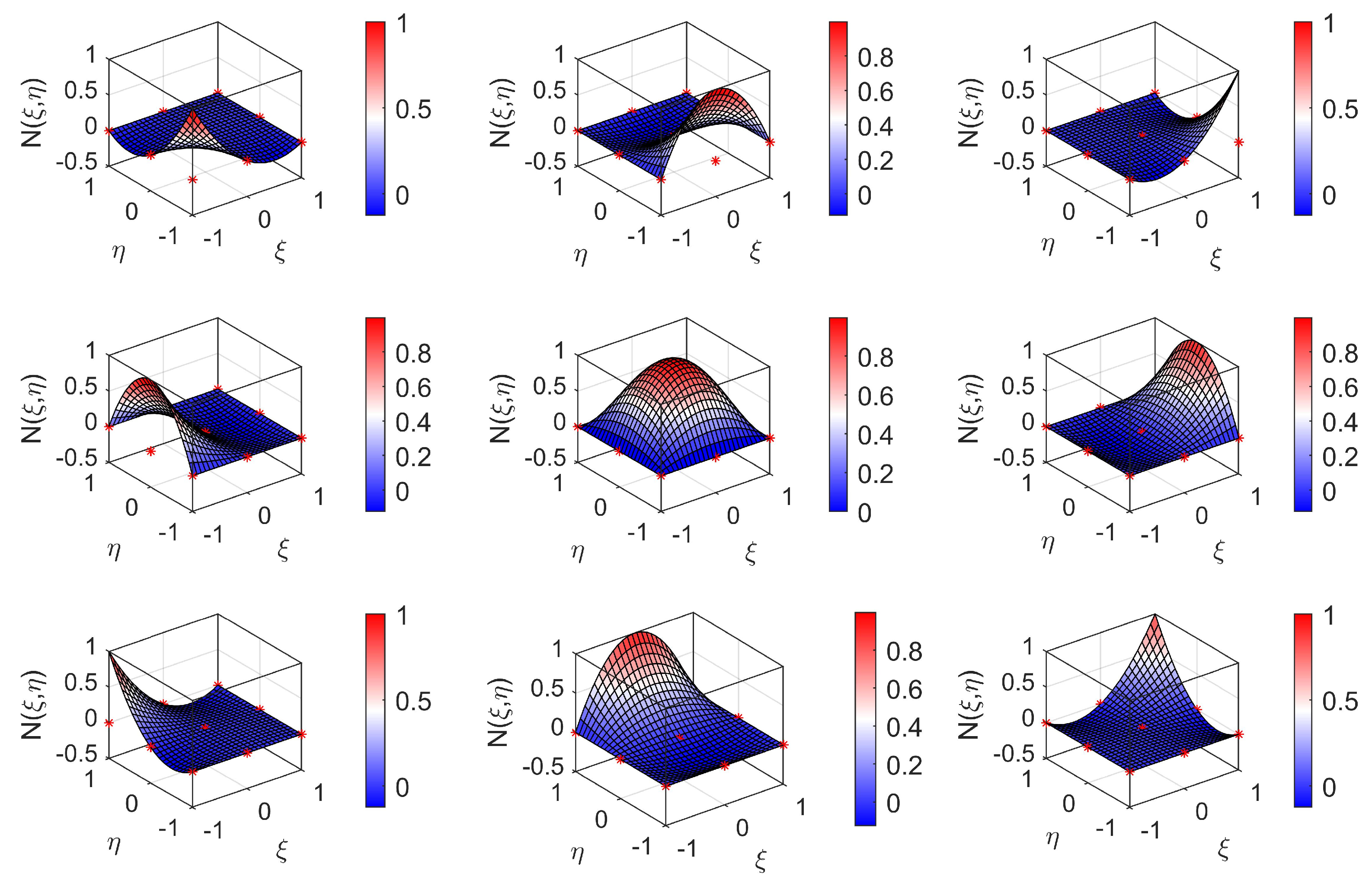
3.2. Legendre Basis Functions

The spectral-element technique is derived from the computational formulation of the finite-element approach, and its numerical accuracy is intricately tied to the order of interpolation basis functions [30]. To obtain high-precision 2D numerical electrical potential, the computational domain is discretized with Gauss–Lobatto–Legendre (GLL) spectral elements. In the case of one dimension, the m-degree GLL interpolation basis functions for sub-element $\xi \in \left[-1,1\right]$ can be expressed as

$${\varphi }_i\left(\xi \right)=\frac{1}{m\left(m+1\right)L_m\left({\xi }_i\right)}\frac{{\xi }^2-1}{\xi -{\xi }_i}{L^{\prime }}_m\left(\xi \right)$$

(16)

where $i=1,2,\cdots ,m+1$, $L_m\left(\xi \right)$ represents the m-degree Legendre orthogonal polynomial and ${L^{\prime }}_m\left(\xi \right)$ is the corresponding first derivative, ${\xi }_i$ is the GLL interpolation point, which is the root of the equation $\left({\xi }^2-1\right){L^{\prime }}_m\left(\xi \right)=0$. Then, the m-degree GLL interpolation basis functions of Equation (16) can be formulated as follows:

$${\varphi }_i\left(\xi \right)=\frac{\left(\xi -{\xi }_1\right)\left(\xi -{\xi }_2\right)\cdots \left(\xi -{\xi }_{i-1}\right)\left(\xi -{\xi }_{i+1}\right)\cdots \left(\xi -{\xi }_{m+1}\right)}{\left({\xi }_i-{\xi }_1\right)\left({\xi }_i-{\xi }_2\right)\cdots \left({\xi }_i-{\xi }_{i-1}\right)\left({\xi }_i-{\xi }_{i+1}\right)\cdots \left({\xi }_i-{\xi }_{m+1}\right)}$$

(17)

On a quadrilateral sub-element, $\xi ,\eta \in \left[-1,1\right]\times \left[-1,1\right]$, the 2D GLL basis functions can be defined by

$$\begin{array}{l}{N}_{ij}\left(\xi ,\eta \right)={\varphi }_i\left(\xi \right){\varphi }_j\left(\eta \right)\\ \hspace{1em}\hspace{1em}\hspace{1em}=\frac{\left(\xi -{\xi }_1\right)\cdots \left(\xi -{\xi }_{i-1}\right)\left(\xi -{\xi }_{i+1}\right)\cdots \left(\xi -{\xi }_{m_1+1}\right)}{\left({\xi }_i-{\xi }_1\right)\cdots \left({\xi }_i-{\xi }_{i-1}\right)\left({\xi }_i-{\xi }_{i+1}\right)\cdots \left({\xi }_i-{\xi }_{m_1+1}\right)}\times \\ \hspace{1em}\hspace{1em}\hspace{1em}\hspace{1em}\hspace{1em}\frac{\left(\eta -{\eta }_1\right)\cdots \left(\eta -{\eta }_{j-1}\right)\left(\eta -{\eta }_{j+1}\right)\cdots \left(\eta -{\eta }_{m_2+1}\right)}{\left({\eta }_j-{\eta }_1\right)\cdots \left({\eta }_j-{\eta }_{j-1}\right)\left({\eta }_j-{\eta }_{j+1}\right)\cdots \left({\eta }_j-{\eta }_{m_2+1}\right)}\end{array}$$

(18)

Therefore, we obtain a polynomial expansion in $\left(\xi ,\eta \right)$ involving $\left(m_1+1\right)\times \left(m_2+1\right)$ coefficients. For instance, in the cases of $m_1=2$ and $m_2=2$, Figure 3 shows the 2D basis functions of the 2 degrees. It consists of 9 basis functions, with the locations of the maximum value corresponding to the interpolation nodes.

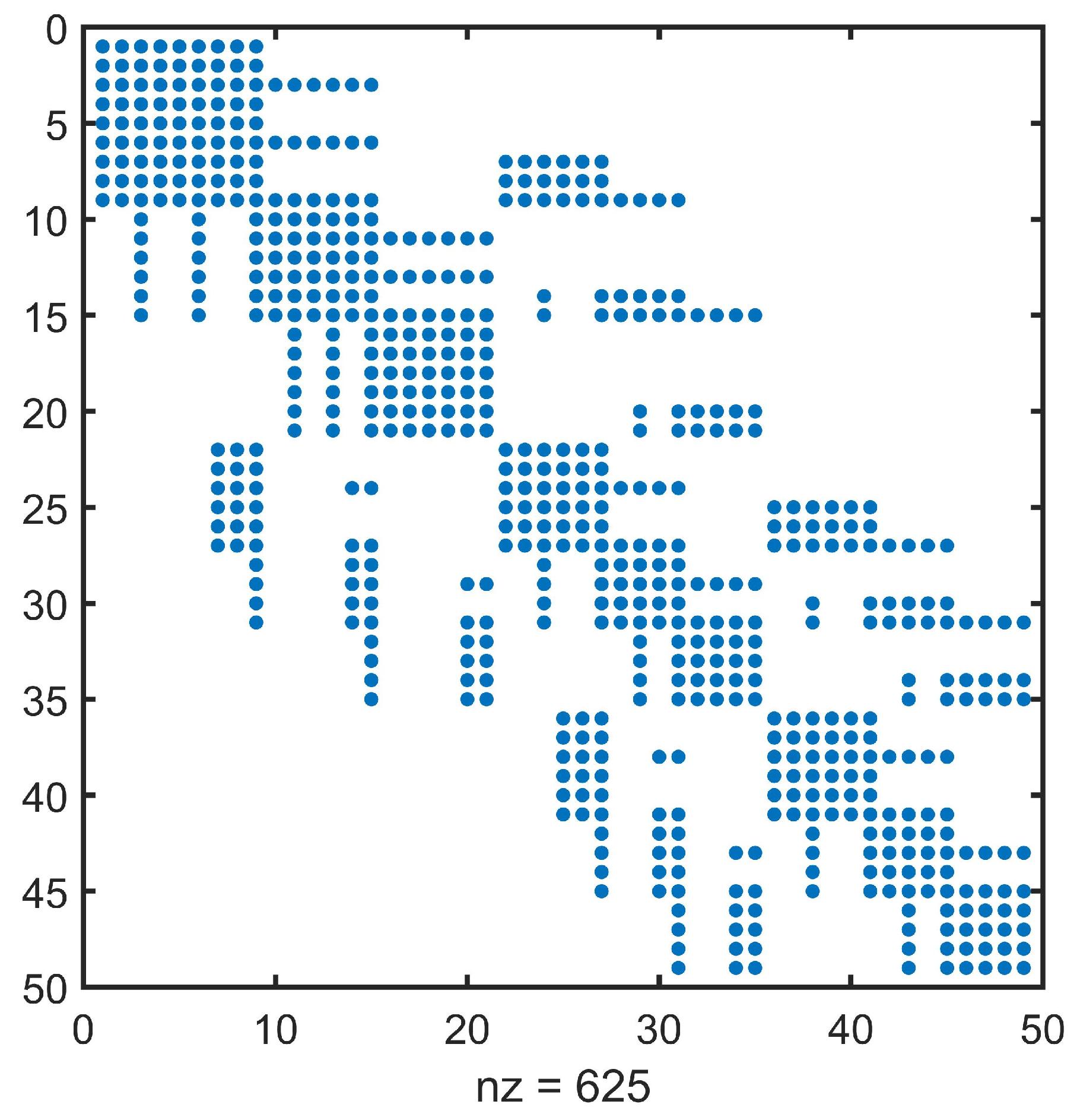
3.3. Legendre Spectral-Element Equation

The spectral-element method requires the mapping of a physical sub-element onto a reference parent element, enabling the computation of the element coefficient matrix within the reference element. Figure 4 provides a mapping example that illustrates the relationship between the $\left(x,z\right)$-coordinate in 2D Legendre spectral element and the normalized $\left(\xi ,\eta \right)$ coordinate with $\xi ,\eta \in \left[-1,1\right]\times \left[-1,1\right]$.

The derivatives and area in the $\left(x,z\right)$-coordinate system, as shown in Equation (15), can be converted to the $\left(\xi ,\eta \right)$-coordinate system using the following transformation:

$$\mathrm{d}x\mathrm{d}z=\left|\begin{array}{l}\frac{\partial x}{\partial \xi }\frac{\partial z}{\partial \xi }\\ \frac{\partial x}{\partial \eta }\frac{\partial z}{\partial \eta }\end{array}\right|\mathrm{d}\xi \mathrm{d}\eta =\left|J\right|\mathrm{d}\xi \mathrm{d}\eta$$

(19)

where $J$ represents the Jacobian matrix of coordinate transformation.

The first integral term in Equation (15) can be expressed as follows:

$$\begin{array}{l}{\displaystyle {\iint }_e\frac{1}{2}\sigma {\left(\nabla U\right)}^2\mathrm{d}x\mathrm{d}z}={\displaystyle {\iint }_e\frac{1}{2}\sigma \left[{\left(\frac{\partial U}{\partial x}\right)}^2+{\left(\frac{\partial U}{\partial z}\right)}^2\right]\mathrm{d}x\mathrm{d}z}\\ \hspace{1em}\hspace{1em}\hspace{1em}\hspace{1em}\hspace{1em}\hspace{1em}\hspace{1em}={\displaystyle {\iint }_e\frac{1}{2}\sigma U_e^T\left[\left(\frac{\partial N}{\partial x}\right){\left(\frac{\partial N}{\partial x}\right)}^T+\left(\frac{\partial N}{\partial z}\right){\left(\frac{\partial N}{\partial z}\right)}^T\right]U_e\mathrm{d}x\mathrm{d}z}\\ \hspace{1em}\hspace{1em}\hspace{1em}\hspace{1em}\hspace{1em}\hspace{1em}\hspace{1em}=\frac{1}{2}{U}_e^T{K}_{1e}{U}_e\end{array}$$

(20)

where

$$\begin{array}{l}{K}_{1e}={\displaystyle {\iint }_e\sigma \left[\left(\frac{\partial N}{\partial x}\right){\left(\frac{\partial N}{\partial x}\right)}^T+\left(\frac{\partial N}{\partial z}\right){\left(\frac{\partial N}{\partial z}\right)}^T\right]\mathrm{d}x\mathrm{d}z}\\ \hspace{1em} ={\displaystyle {\int }_{-1}^1{\displaystyle {\int }_{-1}^1\sigma \left(\frac{\partial N_i}{\partial \xi }\frac{\partial \xi }{\partial x}\right)\left(\frac{\partial N_j}{\partial \xi }\frac{\partial \xi }{\partial x}\right)\left|J\right|\mathrm{d}\xi \mathrm{d}\eta }}+{\displaystyle {\int }_{-1}^1{\displaystyle {\int }_{-1}^1\sigma \left(\frac{\partial N_i}{\partial \eta }\frac{\partial \eta }{\partial z}\right)\left(\frac{\partial N_j}{\partial \eta }\frac{\partial \eta }{\partial z}\right)\left|J\right|\mathrm{d}\xi \mathrm{d}\eta }}\end{array}$$

The second integral term in Equation (15) is simplified as

$${\displaystyle {\iint }_e\frac{1}{2}{\lambda }^2\sigma U^2\mathrm{d}x\mathrm{d}z}=\frac{1}{2}{\lambda }^2\sigma U_e^T{\displaystyle {\iint }_{e}N{N}^T\mathrm{d}x\mathrm{d}z{U}_e}=\frac{1}{2}{U}_e^T{K}_{2e}{U}_e$$

(21)

where $K_{2e}={\lambda }^2\sigma {\displaystyle {\iint }_{e}N{N}^T\mathrm{d}x\mathrm{d}z}={\lambda }^2\sigma {\displaystyle {\int }_{-1}^1{\displaystyle {\int }_{-1}^1{N}_i{N}_j\left|J\right|\mathrm{d}\xi \mathrm{d}\eta }}$.

The third integral term in Equation (15) is simplified as

$${\displaystyle {\iint }_e-I\delta \left(x-x_s\right)\delta \left(z-z_s\right)U\mathrm{d}x\mathrm{d}z}=-\frac{1}{2}I{U}_s.$$

(22)

Only the particular point in the current source can contribute to the integration in Equation (22).

The fourth term in Equation (15) is a line integral, and can be written as

$${\displaystyle {\iint }_{\mathsf{\Gamma }e}\frac{1}{2}\sigma \frac{\lambda K_1\left(\lambda r\right)\cos \left(r,n\right)}{K_0\left(\lambda r\right)}{U}^2\mathrm{d}l}=\frac{1}{2}{U}_e^T{K}_{3e}{U}_e$$

(23)

where $K_{3e}$ can be obtained with a one-dimensional integration.

By aggregating all element integrals and combining Equations (20)–(23), the spectral-element linear equation can be expressed as follows:

$$KU=p$$

(24)

where $K={\displaystyle \sum _{i=1}^{N_e}{K}_{1e}}+{\displaystyle \sum _{i=1}^{N_e}{K}_{2e}}+{\displaystyle \sum _{i=1}^{N_e}{K}_{3e}}$ is a coefficient matrix comprising the wavenumber and the conductivity parameters, and $N_e$ represents the total number of discrete elements. The vector p in Equation (24) is associated with the current point source. Within each spectral element, GLL quadrature, as described in Appendix A, is employed. Figure 5 displays the distribution of sparse elements for a 4 × 4 mesh with polynomial degrees $m_1=2$ and $m_2=2$ (just for illustration purposes). In forward modeling, the large linear system is solved by the ILU-BICGSTAB iterative method [31], which combines a bi-conjugate gradient stabilization algorithm [32] with an incomplete LU decomposition [33].

3.4. Calculation of the Apparent Resistivity Response

After solving Equation (24), we will obtain the discrete electrical potentials $U\left(x,\lambda ,z\right)$ in the wavenumber domain, which can then be transformed into the space-domain electrical potential, $u\left(x,y,z\right)$, through a Fourier inverse transform. The formula for the corresponding inverse transform at the profile (y = 0) can be expressed as follows:

$$u\left(x,0,z\right)=\frac{2}{\pi }{\displaystyle {\int }_0^{+\infty }U\left(x,\lambda ,z\right)\mathrm{d}\lambda }$$

(25)

By utilizing numerical integration, Equation (25) can be reformulated as

$$u\left(r\right)\approx {\displaystyle \sum _{i=1}^N{g}_{i}U\left(r,{\lambda }_i\right)}$$

(26)

where $r=\sqrt{x^2+z^2}$ denotes the distance between the observing position and the current point source, ${\lambda }_i$ signifies the values of discrete wavenumbers, $g_i$ denotes the corresponding weighting coefficient, and N represents the number of discrete wavenumbers. We employ the optimization technique proposed by Xu et al. [34] to determine the appropriate wavenumbers.

Table 1. Six-point wavenumbers, ${\lambda }_i$, and their corresponding weighting coefficients, $g_i$.

i	${\mathit{\lambda }}_{\mathit{i}}$	${\mathit{g}}_{\mathit{i}}$
1	0.0113218	0.0176814
2	0.0601482	0.0486791
3	0.1856957	0.1227978
4	0.5151699	0.3351368
5	1.5271465	1.1654942
6	6.4249320	7.9156312

presents the six-point wavenumbers utilized for converting the wavenumber-domain potential into the space domain.

If there are two current (source) electrodes, the potential is the superposition of the effects from both. Then, the apparent resistivity can be expressed as

$${\rho }_a=G\frac{\Delta u}{I}$$

(27)

where G denotes the geometric factor defined by the geometrical spacings between electrodes, and $\Delta u$ represents the space-domain electrical potential difference, where each potential is the superposition of the effects from both current sources.

4. Accuracy Analysis of the Numerical Algorithm

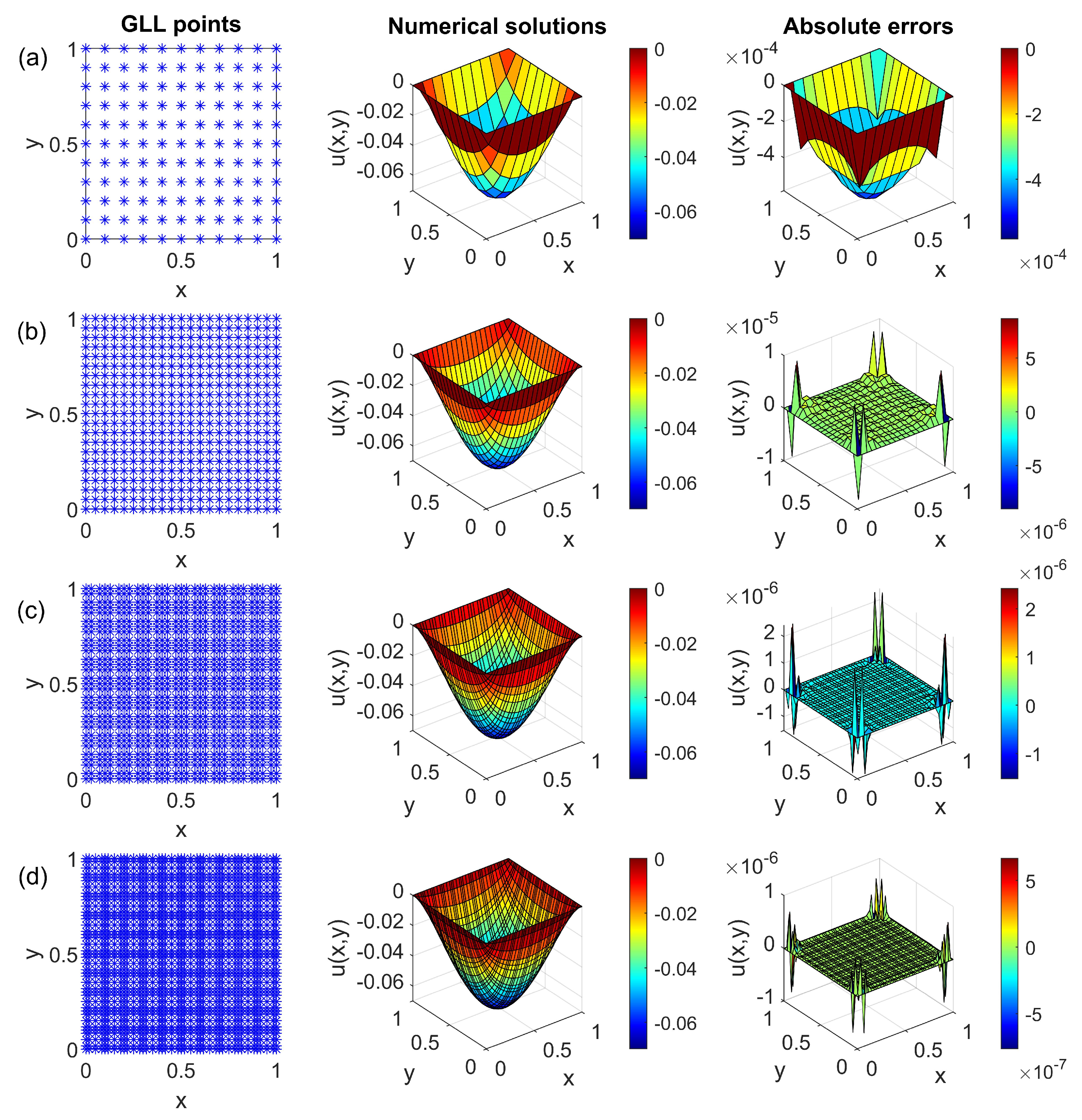
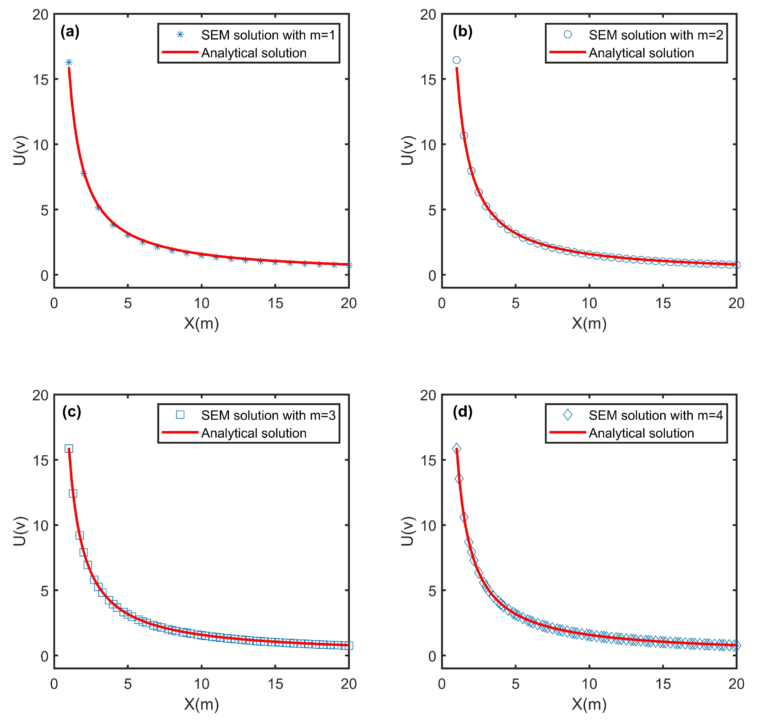
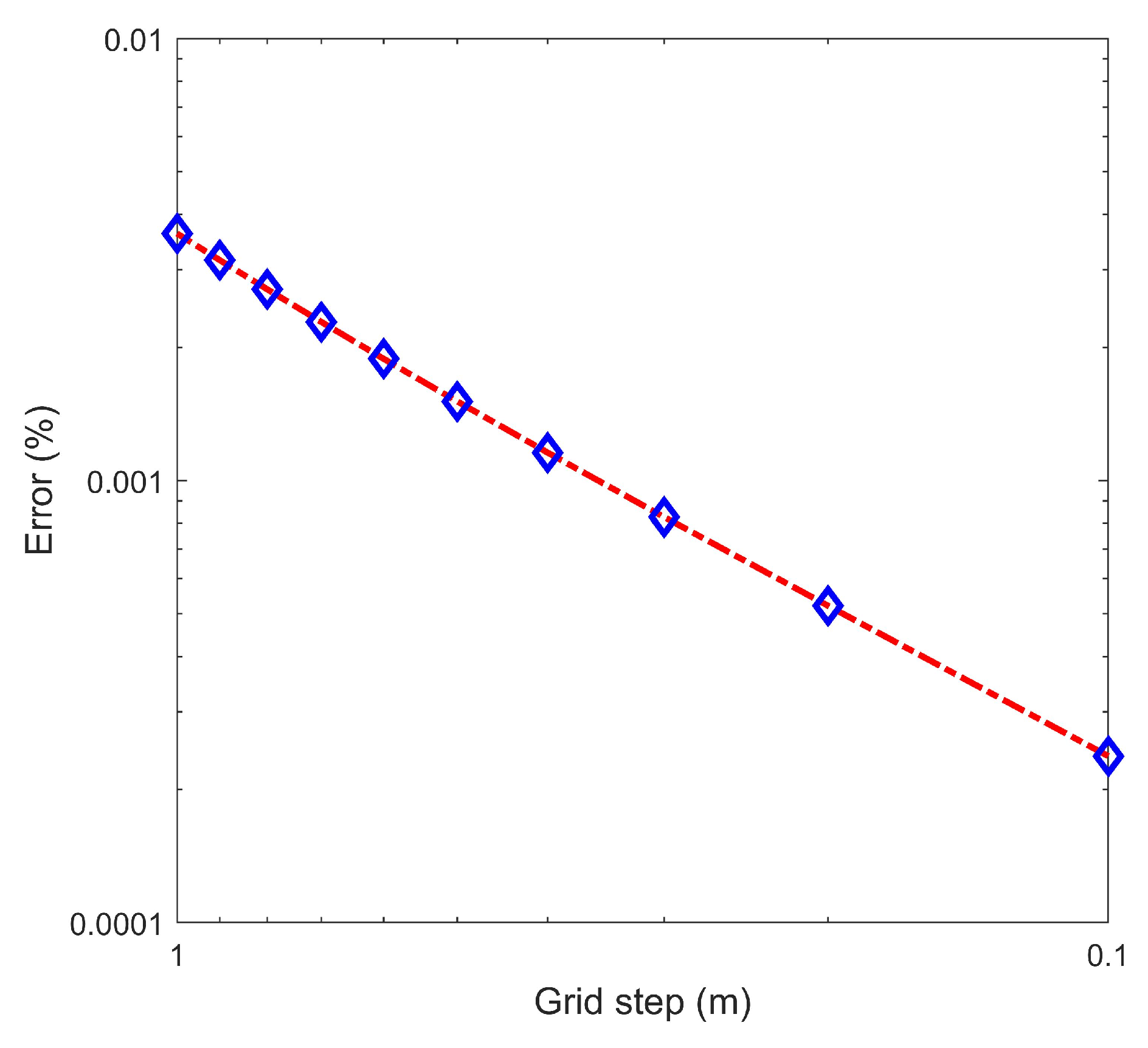
4.1. Two-Dimensional Helmholtz Equation with a Homogeneous Dirichlet Boundary

To test the accuracy of our Legendre spectral-element technique, we considered a two-dimensional Helmholtz equation subject to homogeneous Dirichlet boundary conditions:

$$\frac{{\partial }^{2}u}{\partial x^2}+\frac{{\partial }^{2}u}{\partial y^2}-u=1$$

(28)

Its series solution can be written as

$$\tilde{u}\left(x,y\right)=-{\displaystyle \sum _{a=1,3,\cdots }^{\infty }{\displaystyle \sum _{b=1,3,\cdots }^{\infty }\frac{16}{\left(1+{\pi }^2{a}^2+{\pi }^2{b}^2\right)}\frac{1}{ab{\pi }^2}\sin \left(a\pi x\right)\sin \left(b\pi y\right)}}$$

(29)

A uniform rectangular mesh with 10 × 10 elements is used to discrete the computational domain $\mathsf{\Omega }=\left[0,1\right]\times \left[0,1\right]$. Figure 6 presents the numerical solutions obtained with varying interpolating polynomial degrees. The maximum absolute errors of spectral-element numerical solutions for polynomial degrees 1, 2, 3, and 4 are −5.83E-4, 8.66E-6, 2.42E-6, and 6.66E-7, respectively. The numerical results obtained using the Legendre spectral-element technique can closely match the series analytical solutions, even with a coarse mesh.

4.2. Direct-Current Resistivity Modeling with a Half-Space Model

In order to benchmark the accuracy of the Legendre spectral-element algorithm for 2.5D direct-current-resistivity computational modeling, we developed a resistivity model representing a homogeneous half space. The whole computational domain was defined as a 2000 m × 1000 m area, assuming that the earth surface is flat and uniform, and its conductivity value is equal to 0.01 S/m. The current point source was positioned at (0 m, 0 m), and the current of 1 A was applied. For this numerical simulation, we utilized an 80 × 40 grid.

The numerical results of the electrical potentials at the surface are presented in Figure 7. The spatial-domain electrical potentials, obtained using the Legendre spectral-element approach, exhibit a close agreement with the analytical solutions presented in Appendix B. The numerical results demonstrate the high accuracy of the Legendre spectral-element technique in 2.5D direct-current-resistivity computational modeling.

In addition, the relative root-mean-square error is used to measure the overall accuracy of our spectral-element scheme [35]:

$$\mathrm{Error}=\frac{\sqrt{{\displaystyle \sum _{i=1}^{N_x+1}{\displaystyle \sum _{j=1}^{N_y+1}{\left(u_{i,j}-{\tilde{u}}_{i,j}\right)}^2}}}}{\sqrt{{\displaystyle \sum _{i=1}^{N_x+1}{\displaystyle \sum _{j=1}^{N_y+1}{\left({\tilde{u}}_{i,j}\right)}^2}}}}\times 100 \%$$

(30)

where $N$ and $M$ denote the number of observation points in x- and y-directions, respectively, while $u_{i,j}$ and ${\tilde{u}}_{i,j}$ correspond to the numerical solutions and analytical solutions. Figure 8 displays the convergence plot, in log-log scale, of the relative root-mean-square error based on uniform meshes in the x-direction for the homogeneous half-space model. The error decreases as the grid step-size decreases, demonstrating numerical stability with respect to the grid size and further affirming the accuracy of our spectral-element forward algorithm.

5. Model Computations and Discussion

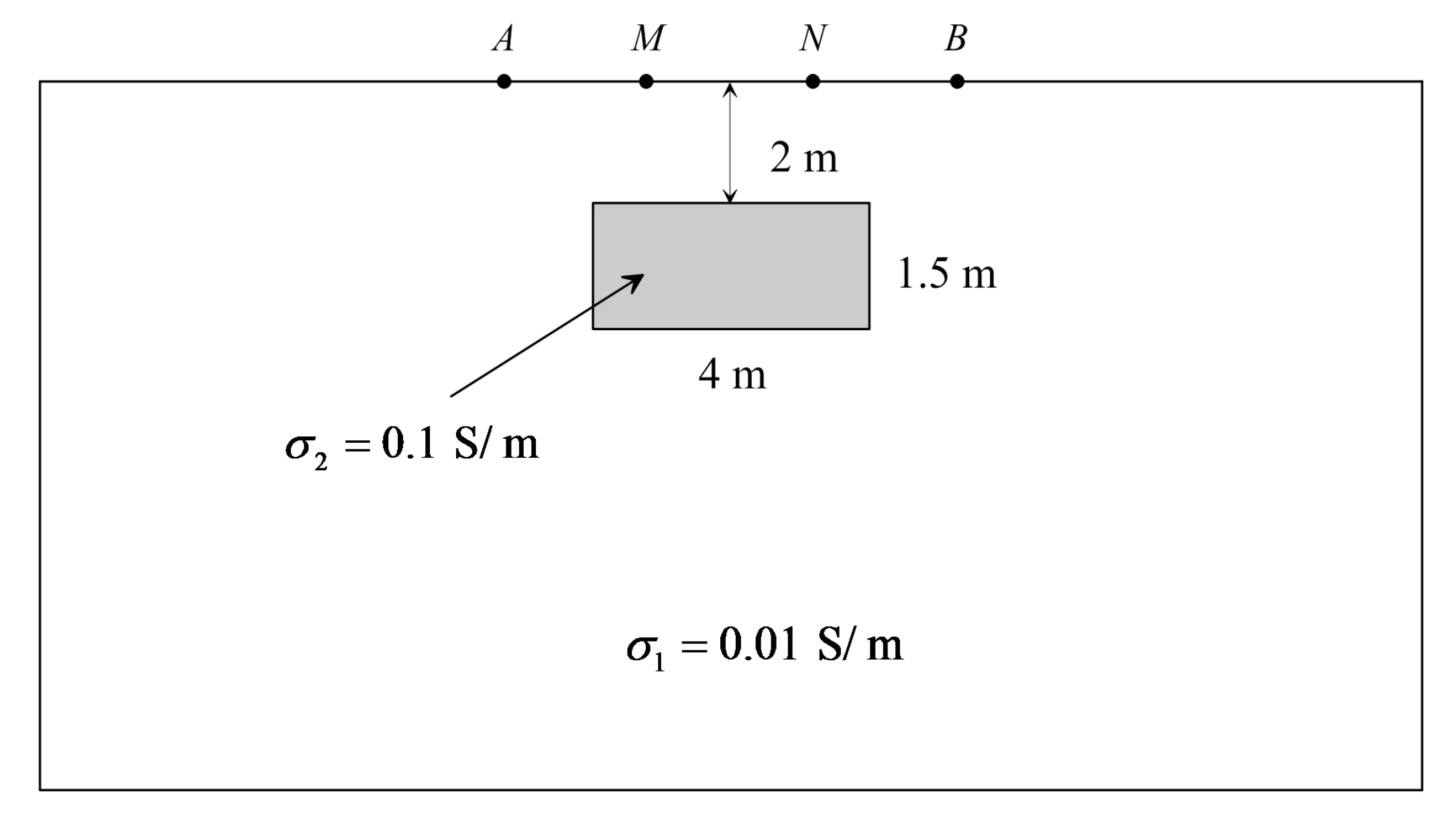
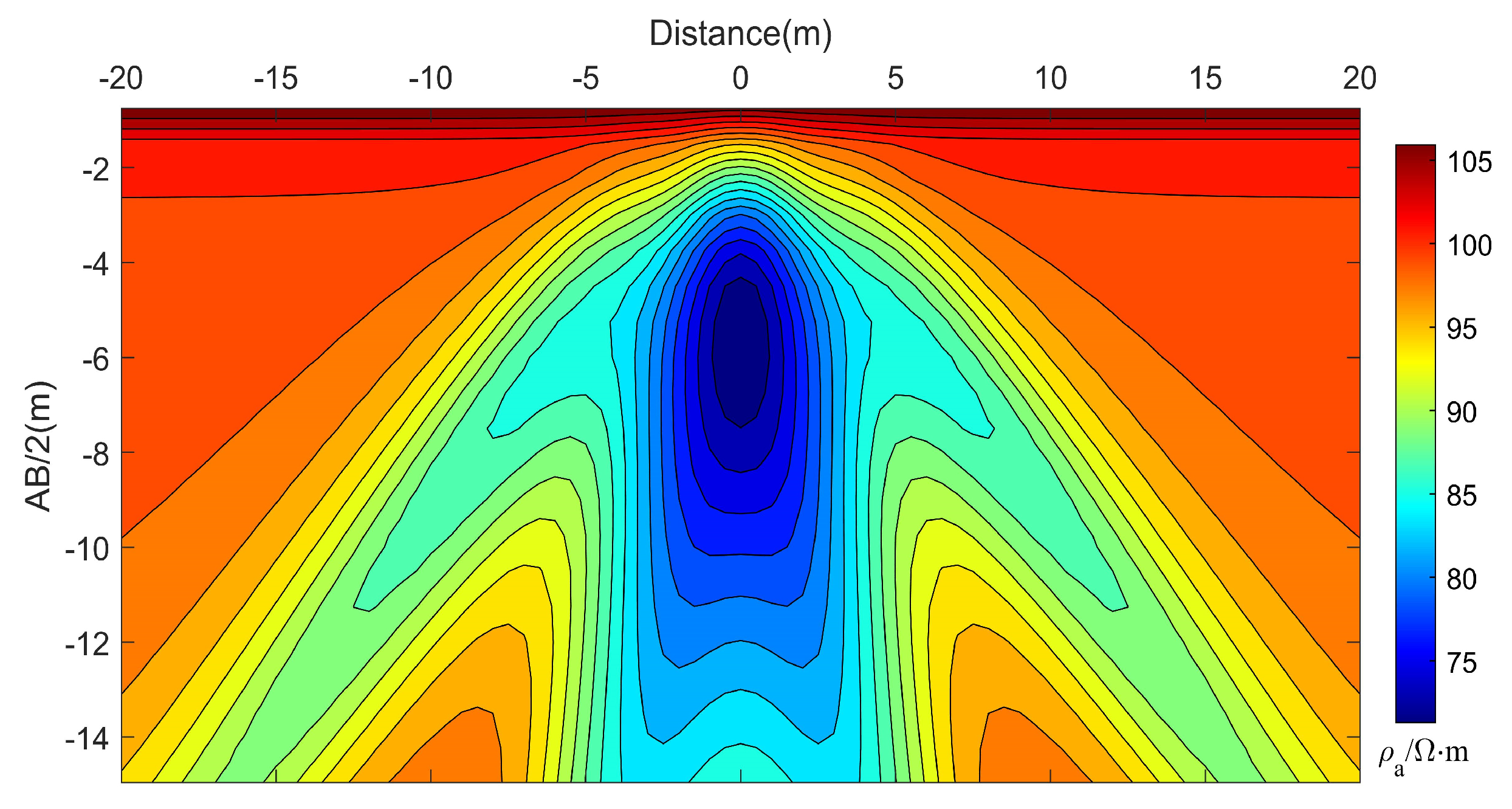
5.1. A 2D Model with a Flat Topography

To illustrate the efficiency of our Legendre spectral-element forward algorithm, we applied a numerical experiment to a simple 2D model, shown in Figure 9. It is a symmetrical, rectangular, conductive body with a conductivity of 0.1 S/m inside a uniform half space. The background conductivity of this 2D model is 0.01 S/m. The width and the thickness of the rectangular body are 4 m and 1.5 m, respectively. The rectangular body is located at a depth of 2 m from the ground surface. Current is delivered through the electrodes A and B, and voltage readings are made with electrodes M and N.

The computational size was set to 100 m × 100 m. The simulation utilized the Wenner-alpha array, and Figure 10 shows the apparent resistivity pseudosection calculated using the spectral-element scheme. The closed contour map enables a qualitative differentiation of the resistivity distribution characteristics of the low-resistivity (or high-conductivity) anomalous body, as well as the accurate identification of its spatial distribution characteristics.

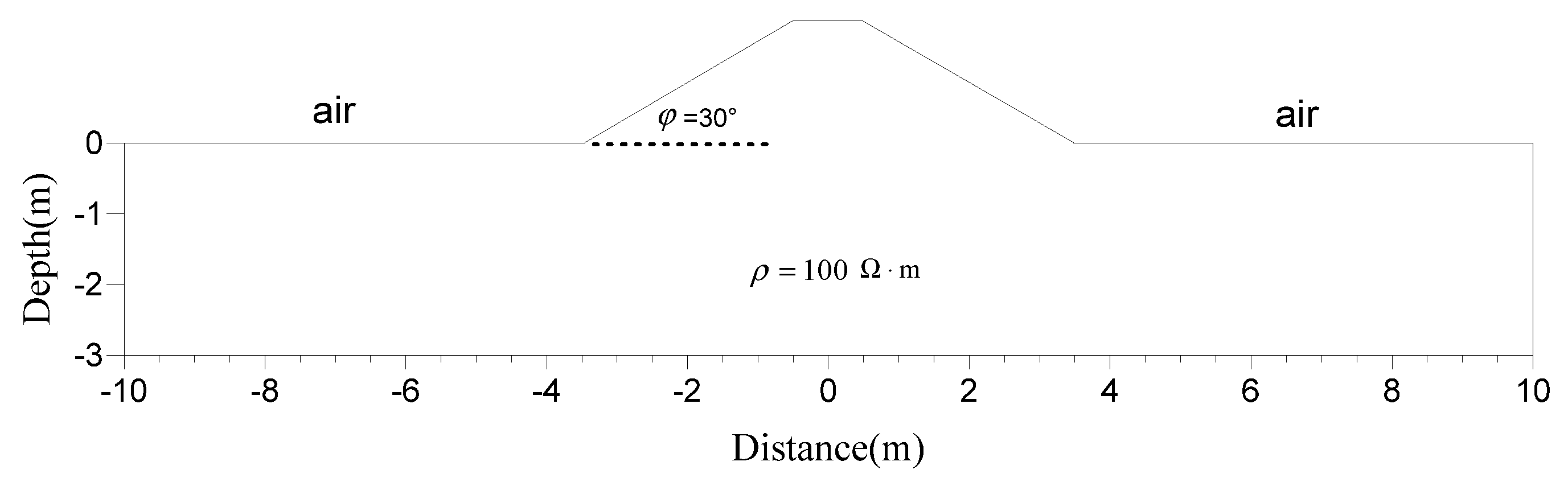
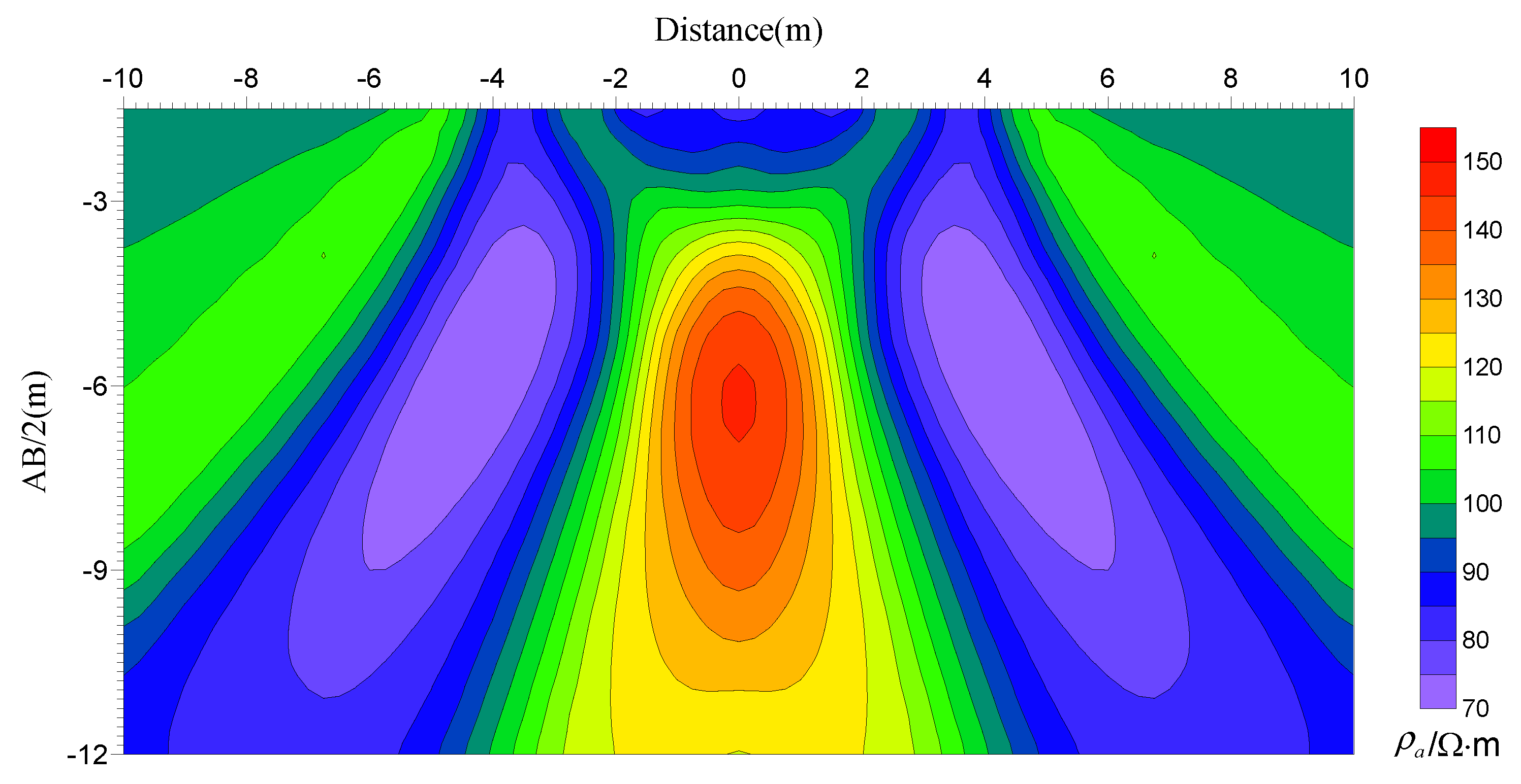
5.2. A Homogeneous Model with a Ridge Topography

In order to simulate the apparent resistivity of the actual undulating terrain, we used the Legendre spectral-element approach for a ridge topographic geo-electrical model [36], as depicted in Figure 11. The undulating ridge terrain has a width of 7 m and an inclination angle of 30°. The horizontal axis represents the horizontal distance and the subsurface medium is homogeneous with a resistivity of 100 $\Omega \cdot \mathrm{m}$.

In our calculation, the entire computational domain is discretized by a non-uniform quadrilateral mesh with 30 × 20 elements, and each element involves 4 GLL nodes in each direction. Figure 12 shows the apparent resistivities obtained using the Legendre spectral-element algorithm for the Wenner-alpha array. It can be seen that the Wenner-alpha array produces a false anomaly of low apparent resistivity below the ridge topography with high false anomalies on either side.

5.3. A Homogeneous Model with a Valley Topography

In Figure 13, a valley topographic model [36] is used to analyze distorted apparent resistivities. The width of the undulating valley terrain is 7 m and the inclination angle is 30°. The medium underground is homogeneous with a resistivity of 100 $\Omega \cdot \mathrm{m}$.

Similarly, the computational domain is discretized by a non-uniform quadrilateral grid with 30 × 20 elements, and each element involves 4 GLL points in each direction. Figure 14 displays the apparent resistivities obtained using the Legendre spectral-element method for the Wenner-alpha array. It can be seen that the Wenner-alpha array in this model produces a false anomaly of high apparent resistivity below the valley topography with low false anomalies on either side.

6. Conclusions

A Legendre spectral-element algorithm has been developed for the first time to solve the 2.5D direct-current-resistivity Helmholtz-type problem. This numerical algorithm combines the complicated topographic flexibility of the FEM with the high-precision approximation of the Chebyshev spectral method or Legendre spectral method. Detailed mathematical formulas for the spectral-element approach are presented, and the numerical approach is implemented in MATLAB code. Numerical experiments of a 2D Helmholtz equation and a resistivity half-space model demonstrate that our proposed spectral-element algorithm can provide a high-precision solution, even when using coarse mesh.

In the direct-current-resistivity exploration, terrain can have a significant impact on the apparent resistivity data and the distortions will vary in different topography models. We have applied the Legendre spectral-element method to simulate the apparent resistivity responses of the ridge and valley topography. Topography effects can be predictable by Legendre spectral-element modeling. In addition, the false anomalies generated by topography must be carefully considered during survey design and data interpretation.

References

1. Yi, M.J.; Kim, J.H.; Son, J.S. Three-dimensional anisotropic inversion of resistivity tomography data in an abandoned mine area. Explor. Geophys. 2011, 42, 7–17. [Google Scholar] [CrossRef]
2. Deng, Z.; Li, Z.; Nie, L.; Zhang, S.; Han, L.; Li, Y. Forward and inversion approach for direct current resistivity based on an unstructured mesh and its application to tunnel engineering. Geophys. Prospect. 2024, 72, 13510. [Google Scholar] [CrossRef]
3. Mitchell, M.A.; Oldenburg, D.W. Using DC resistivity ring array surveys to resolve conductive structures around tunnels or mine-working. J. Appl. Geophys. 2023, 211, 104949. [Google Scholar] [CrossRef]
4. Li, S.; Liu, B.; Nie, L.; Liu, Z.; Tian, M.; Wang, S.; Su, M.; Guo, Q. Detecting and monitoring of water inrush in tunnels and coal mines using direct current resistivity method: A review. J. Rock Mech. Geotech. Eng. 2015, 7, 469–478. [Google Scholar] [CrossRef]
5. Chambers, J.C.; Kuras, O.; Meldrum, P.I.; Ogilvy, R.D.; Hollands, J. Electrical resistivity tomography applied to geologic, hydrogeologic, and engineering investigations at a former waste-disposal site. Geophysics 2006, 71, 231–239. [Google Scholar] [CrossRef]
6. Ammar, A.I.; Kamal, K.A. Detection of shallow and deep conductive zones using direct current resistivity and time-domain electromagnetic methods, west El-Minia, Egypt. Groundw. Sustain. Dev. 2023, 20, 100865. [Google Scholar] [CrossRef]
7. Chang, P.Y.; Doyoro, Y.G.; Lin, D.J.; Puntu, J.M.; Amania, H.H.; Kassie, L.N. Electrical resistivity imaging data for hydrogeological and geological hazard investigations in Taiwan. Data Brief 2023, 49, 109377. [Google Scholar] [CrossRef]
8. Mosaad, A.H.; Farag, M.M.; Wei, Q.; Fahad, A.; Mohamed, S.A.; Hussein, A.S. Integration of electrical resistivity tomography and induced polarization for characterization and mapping of (Pb-Zn-Ag) sulfide deposits. Minerals 2023, 13, 986. [Google Scholar] [CrossRef]
9. Oldenburg, D.W.; Li, Y.; Ellis, R.G. Inversion of geophysical data over a copper gold porphyry deposit: A case history for Mt. Milligan. Geophysics 1997, 62, 1419–1431. [Google Scholar] [CrossRef]
10. Sirota, D.; Shragge, J.; Krahenbuhl, R.; Swidinsky, A.; Yalo, N.; Bradford, J. Development and validation of a low-cost direct current resistivity meter for humanitarian geophysics applications. Geophysics 2022, 87, WA1–WA14. [Google Scholar] [CrossRef]
11. Telford, W.M.; Geldart, L.P.; Sheriff, R.E. Applied Geophysics; Cambridge University Press: Cambridge, UK, 1990. [Google Scholar]
12. Mufti, I.R. Finite-difference resistivity modeling for arbitrarily shaped two-dimensional structures. Geophysics 1976, 41, 62–78. [Google Scholar] [CrossRef]
13. Gernez, S.; Bouchedda, A.; Gloaguen, E.; Paradis, D. AIM4RES, an open-source 2.5D finite difference MATLAB library for anisotropic electrical resistivity modeling. Comput. Geosci. 2020, 135, 104401. [Google Scholar] [CrossRef]
14. Tong, X.; Sun, Y. Fictitious Point Technique Based on Finite-Difference Method for 2.5D Direct-Current Resistivity Forward Problem. Mathematics 2024, 12, 269. [Google Scholar] [CrossRef]
15. Jahandari, H.; Lelièvre, P.; Farquharson, C.G. Forward modeling of direct-current resistivity data on unstructured grids using an adaptive mimetic finite-difference method. Geophysics 2023, 88, 123–134. [Google Scholar] [CrossRef]
16. Zhou, B.; Greenhalgh, S.A. Finite element three-dimensional direct current resistivity modelling: Accuracy and efficiency considerations. Geophys. J. Int. 2001, 145, 679–688. [Google Scholar] [CrossRef]
17. Yan, B.; Li, Y.; Liu, Y. Adaptive finite element modeling of direct current resistivity in 2-D generally anisotropic structures. J. Appl. Geophys. 2016, 130, 169–176. [Google Scholar] [CrossRef]
18. Ren, Z.Y.; Qiu, L.; Tang, J. 3D direct current resistivity anisotropic modelling by goal-oriented adaptive finite element methods. Geophys. J. Int. 2018, 212, 76–87. [Google Scholar] [CrossRef]
19. Tong, X.; Sun, Y.; Zhang, B. An efficient spectral element method for two-dimensional magnetotelluric modeling. Front. Earth Sci. 2023, 11, 1183150. [Google Scholar] [CrossRef]
20. Gharti, H.N.; Tromp, J.; Zampini, S. Spectral-infinite-element simulations of gravity anomalies. Geophys. J. Int. 2018, 215, 1098–1117. [Google Scholar] [CrossRef]
21. Zou, P.; Cheng, J. Pseudo-spectral method using rotated staggered grid for elastic wave propagation in 3D arbitrary anisotropic media. Geophys. Prospect. 2018, 66, 47–61. [Google Scholar] [CrossRef]
22. Gharit, H.N.; Tromp, J. Spectral-infinite-element simulations of magnetic anomalies. Geophys. J. Int. 2019, 217, 1656–1667. [Google Scholar] [CrossRef]
23. Weiss, M.; Kalscheuer, T.; Ren, Z. Spectral element method for 3-D controlled-source electromagnetic forward modeling using unstructured hexahedral meshes. Geophys. J. Int. 2023, 232, 1427–1454. [Google Scholar] [CrossRef]
24. Zhou, Y.; Zhuang, M.; Shi, L.; Cai, G.; Liu, N.; Liu, Q. Spectral element method with divergence-free constraint for 2.5-D marine CSEM hydrocarbon exploration. IEEE Geosci. Remote Sens. Lett. 2017, 14, 1973–1977. [Google Scholar] [CrossRef]
25. Wang, X.; Yu, T.; Feng, D.; Ding, S.; Li, B.; Liu, Y.; Feng, Z. A high-efficiency spectral element method based on CFS-PML for GPR numerical simulation and reverse time migration. IEEE J. Sel. Top. Appl. Earth Obs. Remote Sens. 2023, 16, 1232–1243. [Google Scholar] [CrossRef]
26. Ke, Z.; Liu, L.; Huang, L.; Zhao, Z.; Ji, Y.; Liu, X.; Fang, G. An efficient 2.5-D forward algorithm based on the spectral element method for airborne transient electromagnetics data. Geophys. Prospect. 2023, 71, 1056–1069. [Google Scholar] [CrossRef]
27. Spitzer, K. A 3-D finite-difference algorithm for DC resistivity modelling using conjugate gradient methods. Geophys. J. Int. 1995, 123, 903–914. [Google Scholar] [CrossRef]
28. Penz, S.; Chauris, H.; Donno, D.; Mehl, C. Resistivity modelling with topography. Geophys. J. Int. 2013, 194, 1486–1497. [Google Scholar] [CrossRef]
29. Pozrikidis, C. Introduction to Finite and Spectral Element Methods Using MATLAB; Chapman and Hall Press: New York, NY, USA, 2014. [Google Scholar]
30. Lee, J.H.; Liu, Q.H. An efficient 3-D spectral-element method for Schrodinger equation in nanodevice simulation. IEEE Trans. Comput.-Aided Des. Integr. Circuits Syst. 2005, 24, 1848–1858. [Google Scholar] [CrossRef]
31. Tong, X.; Sun, Y.; Huang, J.; Liu, J. High-accuracy gravity field and gravity gradient forward modelling based on 3D vertex-centered finite-element algorithm. J. Cent. South Unive. 2024, 31, 1–12. [Google Scholar] [CrossRef]
32. Chen, J.; Haber, E.; Oldenburg, D.W. Three-dimensional numerical modelling and inversion of magnetometric resistivity data. Geophys. J. Int. 2002, 149, 679–697. [Google Scholar] [CrossRef]
33. Pan, K.; Wang, J.; Hu, S.; Ren, Z.; Cui, T.; Guo, R.; Tang, J. An efficient cascadic multigrid solver for 3-D magnetotelluric forward modelling problems using potentials. Geophys. J. Int. 2022, 230, 1834–1851. [Google Scholar] [CrossRef]
34. Xu, S.Z.; Duan, B.C.; Zhang, D.H. Selection of the wavenumbers k using an optimization method for the inverse Fourier transform in 2.5D electrical modeling. Geophys. Prospect. 2000, 48, 789–796. [Google Scholar] [CrossRef]
35. Wang, X.; Zhao, D.; Liu, J.; Zhang, Q. Efficient 2D modelling of magnetic anomalies using NUFFT in the Fourier domain. Pure Appl. Geophys. 2022, 179, 2311–2325. [Google Scholar] [CrossRef]
36. Tsourios, P.E.; Szymanski, J.E.; Tsokas, G.N. The effect of terrain topography on commonly used resistivity arrays. Geophysics 1999, 64, 1357–1363. [Google Scholar] [CrossRef]
Figure 1. Schematic diagram of the two-dimensional geo-electrical model. Red inverted triangle represents the location of the current source.
Mathematics 12 01864 g001
Figure 2. Discretization for the 2D computational domain by quadrilateral elements.
Mathematics 12 01864 g002
Figure 3. Graphs of Legendre interpolation functions in part of polynomial degrees m 1 = 2 and m 2 = 2 . Red dots represent GLL points.
Mathematics 12 01864 g003
Figure 4. Schematic diagram of the mapping coordinate system. (a) Mapped quadrilateral element; (b) parent rectangular element.
Mathematics 12 01864 g004
Figure 5. Non-zero value distribution of coefficient matrix formed by the Legendre spectral-element approach.
Mathematics 12 01864 g005
Figure 6. Numerical solutions of the Helmholtz equation using the Legendre spectral-element method with varying interpolating polynomial degrees. (a) m 1 = m 2 = 1 ; (b) m 1 = m 2 = 2 ; (c) m 1 = m 2 = 3 ; (d) m 1 = m 2 = 4 .
Mathematics 12 01864 g006
Figure 7. Comparison of Legendre spectral-element numerical solutions and analytical solutions in homogeneous half spaces using different interpolating polynomial degrees. (a) m 1 = m 2 = 1 ; (b) m 1 = m 2 = 2 ; (c) m 1 = m 2 = 3 ; (d) m 1 = m 2 = 4 .
Mathematics 12 01864 g007
Figure 8. The convergence plot in a log-log scale using the relative root-mean-square error with step sizes.
Mathematics 12 01864 g008
Figure 9. A 2D geo-electrical model with a rectangular body buried in the homogeneous half space.
Mathematics 12 01864 g009
Figure 10. Pseudosection map of the apparent resistivity for the 2D model with the Wenner-alpha array.
Mathematics 12 01864 g010
Figure 11. A homogeneous model with a ridge topography.
Mathematics 12 01864 g011
Figure 12. Pseudosection map of the apparent resistivity for the ridge topography model with the Wenner-alpha array.
Mathematics 12 01864 g012
Figure 13. A homogeneous model with a valley topography.
Mathematics 12 01864 g013
Figure 14. Pseudosection map of the apparent resistivity for the valley topography model with a Wenner-alpha array.
Mathematics 12 01864 g014