A Novel Modified Discrete Differential Evolution Algorithm to Solve the Operations Sequencing Problem in CAPP Systems

Abstract

Operation Sequencing (OS) is one of the most critical tasks in a CAPP system. This process could be modelled as a combinatorial problem where finding a suitable solution within a reasonable time interval is difficult. This work implements a novel Discrete Differential Evolution Algorithm (DDEA) to solve the OS problem, focusing on parts of up to 76 machining operations; the relationships among operations are represented as a directed graph; the contributions of the DDEA are as follows: (1) operates with a discrete representation in the space of feasible solutions; (2) employs mutation and crossover operators to update solutions and to reduce machining and setup costs, (3) possess a local search strategy to achieve better solutions, and (4) integrates a statistical method based on quantiles to measure the quality and likelihood for an achieving a solution. To demonstrate the efficiency and robustness of the DDEA, five prismatic parts with different numbers of machining operations as benchmarks to address the OS problem were selected. The results generated the same OS for parts with a few machining operations (up to 23 machining operations). Conversely, for parts with more machining operations, the DDEA needs more runs to achieve the best solution.

1. Introduction

The computer-aided process planning (CAPP) system is an essential link between computer-aided design (CAD) and computer-aided manufacturing (CAM), which generates detailed instructions to transform the raw material into a finished part. The CAPP systems could be categorised into two types: variant and generative. Variant systems generate plans with group technology (GT), and the second one generates plans automatically; it is constituted by three main modules: characteristic recognition, resource selection, and OS [1,2,3]. The OS is responsible for determining the machining sequence to make a minimum machining cost and time and meet the technological requirements of the part [4,5]. Many researchers have formulated the OS problem in different ways using classical techniques to solve it; however, it is challenging to solve it by applying these kinds of techniques because when the OS problem is mathematically modelled, an NP-hard problem is obtained [6,7,8] that means that is difficult to get an OS optimal, with minimal cost in a reasonable amount of time. In past decades, approximation algorithms like Metaheuristic Algorithms (MAs) have been applied successfully to solve OS problems and find optimal or near-optimal solutions within an acceptable time.

1.1. Literature Review

Some of the most used MAs to tackle the OS problem are neighbourhood algorithms like Simulated Annealing (SA) [9,10] and Tabu Search (TS) [11]. Others based on population, like Genetic Algorithm (GA) [2,6,11,12,13], Particle Swarm Optimisation (PSO) [5,8,14,15,16,17,18], Ant Colony Optimization (ACO) [4,7,19,20], Imperialist Competitive Algorithm (ICA) [21], and Honey Bees Mating Optimization (HBMO) [22].

The GA is the most widely used MA, Zhang et al. [12], presented a novel CAPP model that simultaneously handles the selection of machining resources and the OS, the restrictions imposed by precedence relationships to minimise the total machining cost. The first approach to improving the performance of GA was hybrid algorithms. Li et al. [23] Incorporated the SA neighbourhood strategy after the GA to perform a local search. Li et al. [24] scaled the environment applications and presented a GA that searched optimal or near-optimal plans in simple or distributed manufacturing systems to minimise production costs and processing time. Salehi et al. [13] were among the first authors to apply a pre-algorithm to the main algorithm to generate a Feasible Operation Sequence (FOS); they divided the process planning into two stages: the first uses a GA to develop a FOS, and the second one uses another GA to optimise the machines, tools, and Tool Approach Direction (TAD) for each operation in the sequences. As in a later work, Salehi et al. [25] incorporated an intelligent search strategy instead of the GA in the first stage to generate FOS by reducing the computation time. Other authors, such as Huang et al. [26], focus on algorithms to initialise the population in the feasible domain. They modelled the OS problem as a directed graph and used an adjacency matrix to present the relation in the graph. Likewise, they proposed a technique based on graph theory to initialise the FOS population and used GA to find the best solution. Su et al. [2] used an edge selection coding strategy to generate the GA initial population. Falih et al. [3] propose a constrained permutation algorithm to create a set of FOS to reduce the position part and cutting tools changes as primary criteria. Luo et al. [27] presented a hybrid algorithm with GA that decomposes the search space into simple multi-neighbourhoods and tries to find the best sequence in each subspace generated. It is one of the first authors to use a GA for a complex part that needs 76 manufacturing operations. Other authors add a technique to avoid infeasible populations and a strategy to improve the search. Huang et al. [28] Represent an FOS with a directed graph and hybrid algorithm between GA-SA, which is applied to find the best plan for a complex part with 46 operations. Dou et al. [6] presented the Path-Relinking Genetic Algorithm (PR-GA), which generates a feasible solution using an approach based on a directed graph; the GA uses their operators (mutate and crossover) to ensure feasibility, and the (Path-Relinking) PR is a local search strategy to avoid local minima.

Other popular MAs applied to solve the OS problem are those inspired by the socio-cooperative behaviour of species. The PSO was the first algorithm of its kind. Dou et al. [8] classified the PSO into two main approaches; the first one [5,14,15,29] works with a real representation to search the optimal OS by using the canonical operators proposed by Kennedy et al. [30]. The second approach consists of representing the OS with an integer representation, where the canonical operators were redesigned to handle this kind of representation [1,17]. The second approach performs better than these because the search space is reduced in the discrete representation since the discrete is smaller than the continuous one [8,31].

The ACO is an algorithm based on cooperative behaviour; the first author to use this approach to solve the OS problem was Liu et al. [7]; they modelled it as a constraint travelling salesman problem; in this analogy, the cities are the features of the part, the weights of the cities are the cost for machining processes (machine cost and tool cost). The distances between them are the cost of preparation processes (machine changing, tool changing, and setup changing). Similarly, Wang et al. [20] presented the OS problem as a weighted directed graph and applied the ACO approach to find the best OS, which is represented by a path where all the nodes must be visited. Hu et al. [19] represent the OS problem as an operation precedence graph in which the constrained relationships are divided into precedence constraint relationships and clustering constraint relationships. The first determines the order of operations, and the second ensures the accuracy of the part. They added solution updating methods and local search mechanisms to the algorithm to avoid falling into local minima.

Once the MAs were analysed, it could be seen that they share similar stages; the most common way to represent the OS problem is with a directed graph since it helps to visualise the relationships between the operations through a matrix $n\times n$ where $n$ is the number of operations. To solve the problem, algorithms with integer representation have an advantage over those without because they perform the search in a smaller solution space. One of the best ways to improve the algorithm’s performance is to start the solutions in a feasible space and add an extra algorithm to enhance the search.

In addition, most of the cited works use a precedence constraint handling method to ensure the viability of the plans; they can be classified into three types: (1) penalty, (2) repair, and (3) constraint-satisfied [6,8]. The first adds a penalty cost to the objective function [3,5,11,14,15,16], which increases as more restrictions are violated. This method spends time evaluating invalid plants, and the final plan might not be feasible [11]. The second method [17,21,23,28] uses an algorithm to adjust the infeasible solutions to the feasible domain after applying an updating operator such as mutation or crossover. This method is unreliable, insufficient, and time-consuming when making solutions viable [3]. The constraint-satisfied method works only in the space associated with the FOS; the update operators are specially designed so that the search is carried out in the feasible space [2,3,6]. In [11] mentions another approach called test and generation; this is commonly applied after operators where one or two operations are moved randomly and consists of verifying if the move sequence is valid, then the sequence is retained; otherwise, a new move is performed, its procedure is performed until the solution is feasible.

1.2. Differential Evolution Algorithm for Combinatorial Optimization Problems

The Differential Evolution Algorithm (DEA) created by Storm et al. [32] is an MA population-based that consists of three main phases: mutation, crossover, and selection, which are repeated until a stop criterion is met. Firstly, a population of target solutions is initialised; each target solution generates a mutation solution using three different solutions taken randomly, where one of them is altered by a scaled difference of the other two. A trial solution is generated by combining the elements of the target solution with elements of the mutant solution. Finally, whether the target or its trial solution goes to the next generation is decided. It is essential to highlight that DEA operators are consistently applied to generate new solutions instead of MAs with probabilistic schemas.

Due to its simplicity, easy implementation, reliability, and high performance, it has been successfully adopted by the scientific community [33]. The areas where it has been applied are vast: medicine, operations research, image processing, industrial and electrical engineering, etc. [34]. However, its continuous nature has been an obstacle to applying it directly to combinatorial optimization problems. Two schemes have been reported to tackle this deficiency [33,35]. In the first one, the solution is represented with a vector of integers, and a mapping technique was used to code the integer elements into reals; the evolutionary operators proposed by Storm et al. [32] are applied to update the solutions and then are re-coded to an integer representation and evaluated [35,36,37]. In the second one, in the same way, the solutions are represented directly with a vector of integer elements. Still, instead of updating the solutions with canonical operators (mutation and crossover), these are redesigned to handle the integer elements [33,38]. The main strength of PSO and DEA approaches lies in solving problems of numerical optimisation problems. Both approaches present similar coding schemes in both matches to overcome their deficiency in solving combinatorial optimization problems. Maintaining an integer representation of solutions throughout the search process, i.e., without mapping to a real representation, has advantages because the search space is reduced. The solutions can be kept within the feasible domain without penalty or repair.

1.3. Summary

Although many approaches have been applied to the OS problem with good results, some issues still need attention, mainly the unfeasible OS and the application to complex or part with mid-to-large features. To address the above, we propose a new discrete differential evolution algorithm (DDEA); this approach will handle a discrete representation to reduce the search space and to reduce even further the search remains in the feasible space in this way by increasing the opportunities to achieve the global minima to parts with many features. The target population was created in the feasible space using a variant of topological sort. The mutation and crossover operators were redesigned to handle the discrete solution representation. Both operators combine solutions in each generation to avoid falling into local minima while reducing total production costs. The discrete mutant operator reduces the machine and tool costs, and on the other hand, the discrete crossover reduces the costs generated by the change of machines, tools, and setup. Finally, a local search strategy is incorporated to improve the search in the FOS space. Five parts with different features and operations were taken as case studies to show the DDEA performance.

The remainder of this paper is as follows: in the “Problem formulation” section, the OS problem is stated. The “Discrete differential evolution algorithm for operations sequence problem” section describes the stages that conform to the proposed algorithm. The section “Time Complexity” analyses each DDEA stage’s time complexity using the big O notation. The “Determination of DDEA parameters” section helps find the appropriate values to achieve minimum costs consistently. The section “Case studies and results analysis” describes the five prismatic parts, the experiments carried out, and the results obtained, compared with those found in the literature review. The section “Conclusions and future work” reflects on the topic, and proposals for future works are mentioned.

2. Problem Formulation

The OS in generative CAPP systems must respect the sequence required to achieve the features as long as their manufacturing operations advance. This order is established by manufacturing rules known as precedence constraints, caused by many factors such as the number and type of machines, tooling and fixtures, features, tolerances, and heat treatment available. This research uses the precedence constraints proposed by [5,23]. An operation precedence graph (OPG) represents those in which the nodes are the operations, and the edges indicate a relationship among the operations. Figure 1a shows the OPG with seven operations in which operation Op7 is related to Op1 and Op3; this means that Op7 needs to be done before Op1 and Op3. Another way to represent this OPG is by using a $n\times n$ Boolean adjacent matrix, in which $n$ are all the required operations to manufacture the part. Its elements in a position $\left(i,j\right)$ will be 1 if operations ${op}_i$ and ${op}_j$ have some precedence constraint, and it is 0 otherwise (Figure 1b).

Evaluation Criteria

Most authors select the quantitative criterion for evaluating OS, the production cost, which can be divided into machining and setup costs [7]. The first one is composed of the total machine cost (TMC) and total tool cost (TTC); the second one is formed by the machine change cost (MCC), tool change cost (TCC), and setup change cost (SCC).

Total machine cost is the cost of all the machines used in the sequence; it is calculated as:

$$\mathrm{T}\mathrm{M}\mathrm{C}={\sum }_{i=1}^D{\mathrm{M}\mathrm{C}}_i,$$

(1)

where $D$ is the total number of operations and ${\mathrm{M}\mathrm{C}}_i$ is a constant cost that belongs to the i machine.

Total tool cost is the cost of all the tools used in the sequence; it is calculated as:

$$\mathrm{T}\mathrm{T}\mathrm{C}={\sum }_{i=1}^D{\mathrm{T}\mathrm{C}}_i,$$

(2)

where ${\mathrm{T}\mathrm{C}}_i$ is the constant cost that belongs to the i tool.

Machine change cost: it is needed when the sequence of two neighbouring operations is performed on different machines; it is calculated as:

$$\mathrm{M}\mathrm{C}\mathrm{C}=\mathrm{M}\mathrm{C}\mathrm{C}\mathrm{I}\times \mathrm{N}\mathrm{M}\mathrm{C},$$

(3)

where $\mathrm{M}\mathrm{C}\mathrm{C}\mathrm{I}$ refers to the $\mathrm{M}\mathrm{C}\mathrm{C}$ index, which is a constant value, and $\mathrm{N}\mathrm{M}\mathrm{C}$ is the number of machine changes calculated as:

$$\mathrm{N}\mathrm{M}\mathrm{C}={\sum }_{i=1}^{D-1}{\mathsf{\Omega }}_1\left({\mathrm{M}}_{i+1},{\mathrm{M}}_i\right),$$

(4)

where ${\mathrm{M}}_i$ is the ID of the machine and used to perform the $i$ operation, ${\mathsf{\Omega }}_1\left(x,y\right)$ is a decision variable that indicates if a machine change between neighbouring operations exists.

$${\mathsf{\Omega }}_1\left(x,y\right)=\left\{\begin{array}{c}1,\mathrm{si}x\ne y\\ 0,\mathrm{si}x=y\end{array}\right..$$

(5)

Tool change cost is needed when two neighbouring operations are performed with (a) the same machine and different tools, (b) different machines but the same tools, and (c) different machines and tools. It is calculated as:

$$\mathrm{T}\mathrm{C}\mathrm{C}=\mathrm{T}\mathrm{C}\mathrm{C}\mathrm{I}\times \mathrm{N}\mathrm{T}\mathrm{C},$$

(6)

where $\mathrm{T}\mathrm{C}\mathrm{C}\mathrm{I}$ is the $\mathrm{T}\mathrm{C}\mathrm{C}$ index constant value, and $\mathrm{N}\mathrm{T}\mathrm{C}$ is the number of tool changes calculated as:

$$\mathrm{N}\mathrm{T}\mathrm{C}={\sum }_{i=1}^{D-1}{\mathsf{\Omega }}_2\left({\mathsf{\Omega }}_1\left({\mathrm{M}}_{i+1},{\mathrm{M}}_i\right),{\mathsf{\Omega }}_1\left({\mathrm{T}}_{i+1},{\mathrm{T}}_i\right)\right),$$

(7)

where ${\mathrm{T}}_i$ is the tool ID and it is used to perform the i operation, and ${\mathsf{\Omega }}_2\left(x,y\right)$ comes from Equation (10).

Setup change cost is needed when two neighbouring operations are performed with the following options, the same machine and different TAD, different machines, and same TAD, and both different machine and TAD, it is calculated as:

$$\mathrm{S}\mathrm{C}\mathrm{C}=\mathrm{S}\mathrm{C}\mathrm{C}\mathrm{I}\times \mathrm{N}\mathrm{S}\mathrm{C},$$

(8)

where $\mathrm{S}\mathrm{C}\mathrm{C}\mathrm{I}$ is the $\mathrm{S}\mathrm{C}\mathrm{C}$ index, it is a constant value, and $\mathrm{N}\mathrm{S}\mathrm{C}$ is the number of setup changes, and it is computed as:

$$\mathrm{N}\mathrm{S}\mathrm{C}=1+{\sum }_{i=1}^{D-1}{\mathsf{\Omega }}_2\left({\mathsf{\Omega }}_1\left({\mathrm{M}}_{i+1},{\mathrm{M}}_i\right),{\mathsf{\Omega }}_1\left({\mathrm{T}\mathrm{A}\mathrm{D}}_{i+1},{\mathrm{T}\mathrm{A}\mathrm{D}}_i\right)\right),$$

(9)

where ${\mathrm{T}\mathrm{A}\mathrm{D}}_i$ is the ID of the $\mathrm{T}\mathrm{A}\mathrm{D}$ used to perform the $i$ operation, ${\mathsf{\Omega }}_2$ is a decision variable equal to 0 if the neighbouring operations are performed with the same machine and the same TAD. It will be equal to 1 when the operations are executed with the same machine and different TAD.

$${\mathsf{\Omega }}_2\left(x,y\right)=\left\{\begin{array}{l}0,\mathrm{if}x=y=0\\ 1\hspace{1em}\mathrm{otherwise}\end{array}\right..$$

(10)

The total production cost is calculated by:

$$\mathrm{T}\mathrm{C}={\mathsf{\omega }}_1\mathrm{T}\mathrm{M}\mathrm{C}+{\mathsf{\omega }}_2\mathrm{T}\mathrm{T}\mathrm{C}+{\mathsf{\omega }}_3\mathrm{M}\mathrm{C}\mathrm{C}+{\mathsf{\omega }}_4\mathrm{T}\mathrm{C}\mathrm{C}+{\mathsf{\omega }}_5\mathrm{S}\mathrm{C}\mathrm{C}.$$

(11)

In Equation (11), ${\mathsf{\omega }}_1$–${\mathsf{\omega }}_5$ are weights values that can be 0 or 1, which can be used to customize the process plans [11]. For example, if ${\mathsf{\omega }}_1={\mathsf{\omega }}_2=0$, and ${\mathsf{\omega }}_3={\mathsf{\omega }}_4={\mathsf{\omega }}_5=1$, the preparation cost will only be considered, not the machining cost.

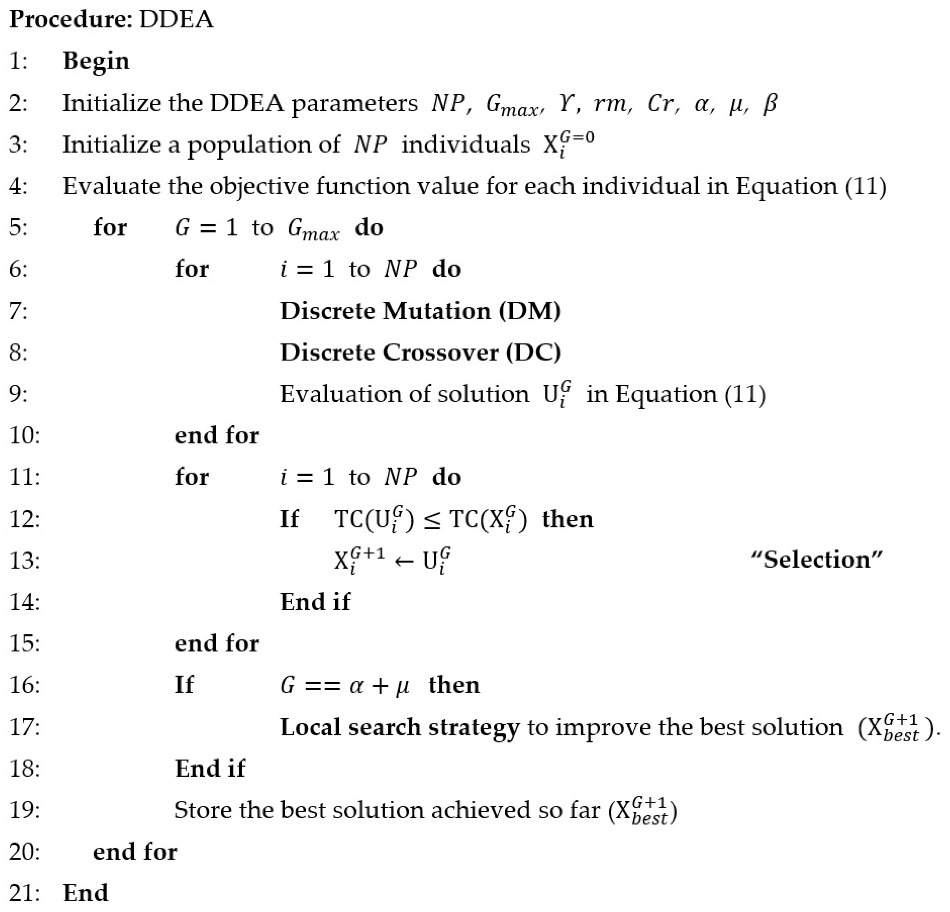
3. Discrete Differential Evolution Algorithm for Operations Sequence Problem

3.1. Description

Due to its discrete nature, the traditional DEA is designed to solve continuous optimization problems; therefore, it cannot be directly applied to solve the OS problem in CAPP systems. This section presents a novel DDEA to solve the operation sequence problem; the details include a solution representation, population initialization, mutation and crossover operators design, selection, and local search strategy, which are described as follows.

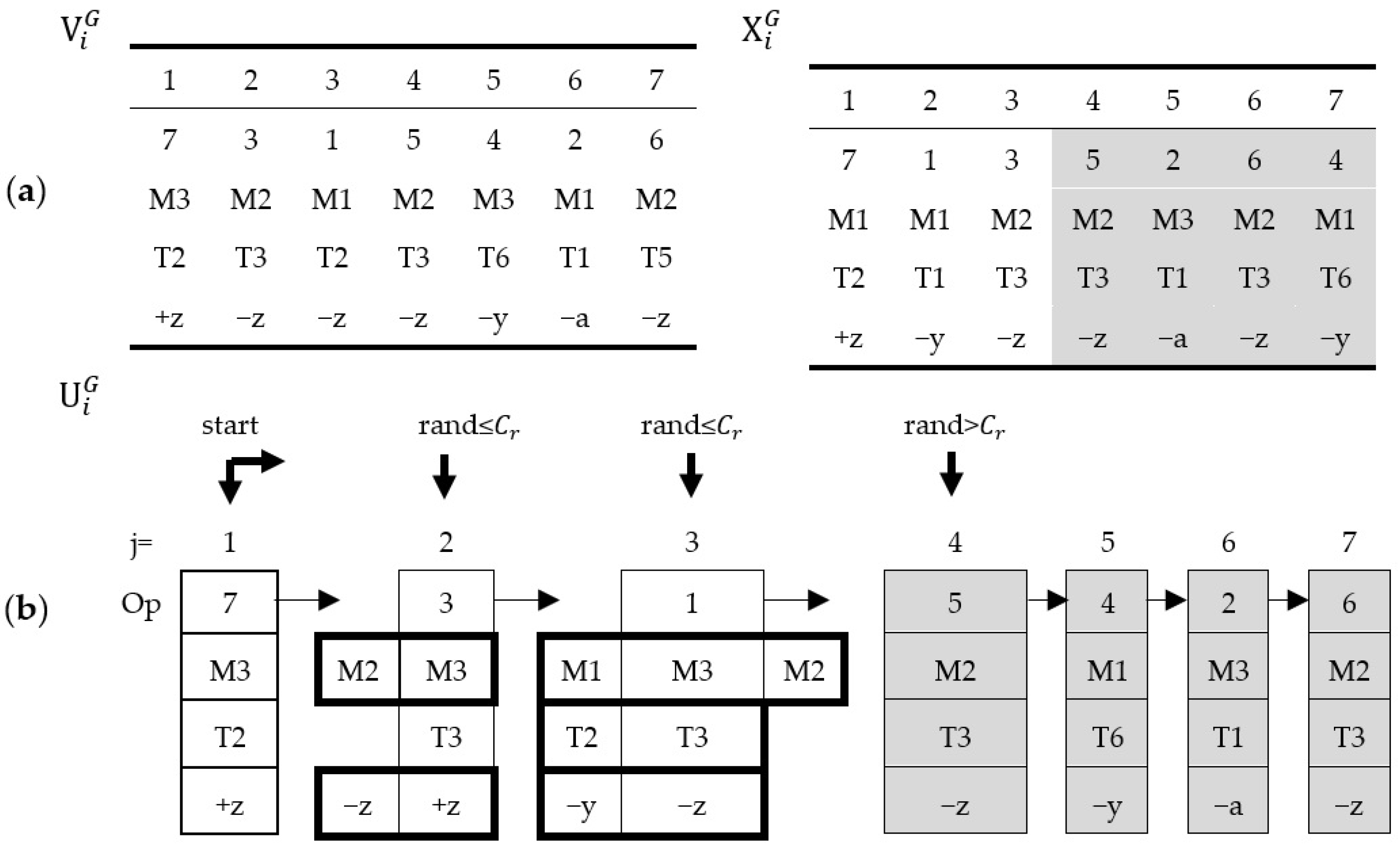
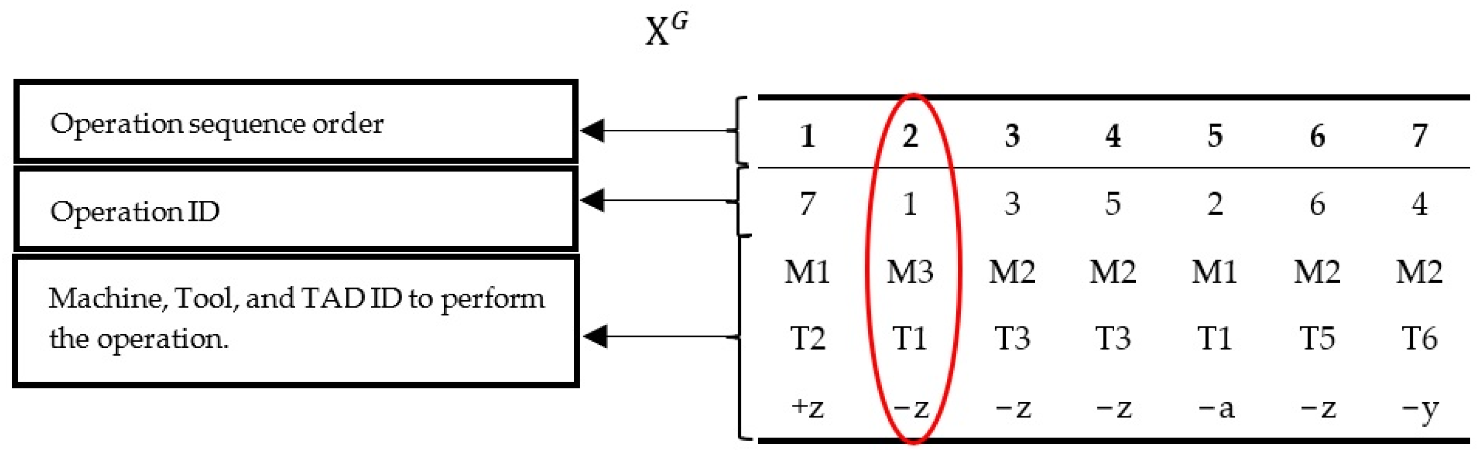
3.2. Solution Representation

In the DDEA process, the candidate solutions represent OS, where each operation in the sequence has its machine, cutting tool, and TAD. A 4 × $D$ rectangular matrix is used to describe it, where $D$ is the number of operations required to make the characteristics of the part. The operations that compose the sequence are placed in the first element of each column, the machine ID in the second, the cutting tool ID in the third, and the TAD ID in the fourth. Figure 2 shows a solution with seven operations where operation one will be the second operation to be performed; this operation will be performed with the machine ID M3, cutting tool ID T1, and TAD ID −z.

3.3. Initialization

The initial population, also called target, is generated by using a variation of topological sort (TS-based representation) proposed by [39]. This method generates a feasible OS starting from a directed graph where a node without precedence constraints is randomly selected and added. To each operation in the sequence, an available machine ID (M), tool ID (T), and TAD ID are randomly assigned. This process is repeated until the population $NP$ is generated.

3.4. Discrete Mutation (DM)

According to the classical DE algorithm, a mutant solution is created in the mutation operator for each target solution by perturbing a base solution with the scaled difference between two solutions randomly selected from the target population. Based on this idea, a discrete mutation operator is designed based on the combination of 1/best and 1/rand strategies.

$${\mathrm{V}}_i^G={\mathrm{X}}_{\mathrm{b}\mathrm{a}\mathrm{s}\mathrm{e}}^G⨂\mathsf{{\rm Y}}⨁\left({\mathrm{X}}_{{\mathrm{r}}_2}^G⊝{\mathrm{X}}_{{\mathrm{r}}_3}^G\right),$$

(12)

where ${\mathrm{X}}_{\mathrm{b}\mathrm{a}\mathrm{s}\mathrm{e}}^G$ is the solution base index, $r_2$ and $r_3$ are indices of the two solutions selected randomly in the range [1, $NP$] to be fulfilled ${\mathrm{b}\mathrm{a}\mathrm{s}\mathrm{e}\ne r}_2\ne r_3\ne i$, $(i=1,2,3,\dots ,NP)$. The mutant factor $\mathsf{{\rm Y}}\in [0,1]$, ${\mathrm{V}}_i^G$ is the mutant solution that corresponds to the target solution ${\mathrm{X}}_i^G$. The definitions of ‘$⨂$’, ‘$⊝$’, and ‘$⨁$’ in Equation (12) are described as follows.

The first operator $‘⨂’$ selects the base solution index using Equation (13).

$${\mathrm{X}}_{\mathrm{b}\mathrm{a}\mathrm{s}\mathrm{e}}^G=\{{\mathrm{X}}_{best}^G,\mathrm{i}\mathrm{f}\mathrm{r}\mathrm{a}\mathrm{n}\mathrm{d}\left(\mathrm{0,1}\right)\le \mathsf{{\rm Y}};\hspace{1em}{\mathrm{X}}_{{\mathrm{r}}_1}^G,\mathrm{o}\mathrm{t}\mathrm{h}\mathrm{e}\mathrm{r}\mathrm{w}\mathrm{i}\mathrm{s}\mathrm{e},$$

(13)

where $best$ is the index of the solution with the lowest value of TC (Equation (11)) in the current generation ($G$), and $r_1$ is the index of a solution selected in the rage [1, $NP$].

The operator ‘$⊝$’ generates the temporal matrix $\mathsf{\Delta }$ that contains operations that are in the same order of solutions with indexes $r_2$ and $r_3$; the machine and tool in this operation will have the minimum TMC and TTC. Its procedure is described as follows:

Step 1:

$\mathsf{\Delta }\leftarrow null$; $nd=1$.

Step 2:

For each operation in the columns ${\mathrm{X}}_{r_2}^G\left(n\right)$ and ${\mathrm{X}}_{r_3}^G\left(n\right)$, were

$n=\mathrm{1,2},3,\dots ,D$.

Step 3:

If the operation in column ${\mathrm{X}}_{r_2}^G\left(n\right)$ is equal to the operation in the column ${\mathrm{X}}_{r_3}^G\left(n\right)$, then, the operation in ${\mathrm{X}}_{r_3}^G\left(n\right)$ is assigned to $\mathsf{\Delta }\left(nd\right)$.

Step 3.1:

If the machine ID in ${\mathrm{X}}_{r_2}^G\left(n\right)$ is equal to machine ID in ${\mathrm{X}}_{r_3}^G\left(n\right)$ then assign the machine ID to column $\mathsf{\Delta }\left(nd\right)$, else,

the cost of the machine ID in the column ${\mathrm{X}}_{r_2}^G\left(n\right)$ and ${\mathrm{X}}_{r_3}^G\left(n\right)$ is obtained.

If the cost of the machine ID in ${\mathrm{X}}_{r_2}^G\left(n\right)$ is less than the cost of the machine ID in ${\mathrm{X}}_{r_3}^G\left(n\right)$, then, the machine ID in ${\mathrm{X}}_{r_2}^G\left(n\right)$ is assigned to column $\mathsf{\Delta }\left(nd\right)$.

elseif, the machine ID in ${\mathrm{X}}_{r_2}^G\left(n\right)$ is greater than the cost of machine ID in ${\mathrm{X}}_{r_3}^G\left(n\right)$, then, the machine ID in ${\mathrm{X}}_{r_3}^G\left(n\right)$ is assigned to column $\mathsf{\Delta }\left(nd\right)$.

else the machine ID is selected randomly.

Step 3.2:

Carry out the same procedure in step 3.1 for the tool ID.

Step 3.3:

If the TAD ID in column ${\mathrm{X}}_{r_2}^G\left(n\right)$ is equal to TAD ID in column ${\mathrm{X}}_{r_3}^G\left(n\right)$, then assign TAD ID in ${\mathrm{X}}_{r_2}^G\left(n\right)$ to column $\mathsf{\Delta }\left(nd\right)$, else,

Select one TAD ID randomly between ${\mathrm{X}}_{r_2}^G\left(n\right)$ and ${\mathrm{X}}_{r_3}^G\left(n\right)$, and assign to $\mathsf{\Delta }\left(nd\right).$

$nd=nd+1$

Step 4:

output $\mathsf{\Delta }$

The last operator ‘$⨁$’, calculate ${\mathrm{V}}_i^G={\mathrm{X}}_{base}^G⨁\mathsf{\Delta }$, and is generated as follows:

Step 1:

If $\mathsf{\Delta }$ has all the operations, then ${\mathrm{V}}_i^G\leftarrow \mathsf{\Delta }$.

Step 2:

Elseif $\mathsf{\Delta }$ is null, then ${\mathrm{V}}_i^G\leftarrow {\mathrm{X}}_{aux}^G$.

Step 3:

Elseif $\mathsf{\Delta }$ have between 1 and $D-1$ operations, then.

Step 3.1: 

${\mathrm{X}}_{ref}^G\leftarrow {\mathrm{X}}_{base}^G$.

Step 3.2: 

Delete the columns of ${\mathrm{X}}_{ref}^G$ whose operations are in $\mathsf{\Delta }$.

Step 3.3: 

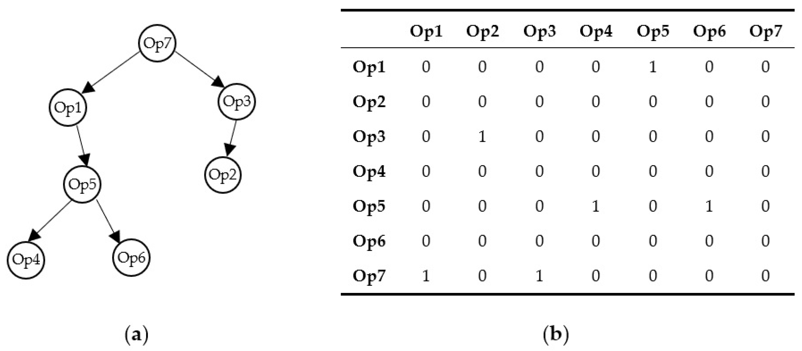
Set $p\leftarrow 1$; $q\leftarrow 1$; $k\leftarrow 1$.

Step 3.4: 

While $k\le D$, then

Step 3.5: 

Verify if the operations in $\mathsf{\Delta }\left(p\right)$ and ${\mathrm{X}}_{ref}^G\left(q\right)$ have restrictions.

Step 3.6: 

If the operation in $\mathsf{\Delta }\left(p\right)$ has no restrictions, then,

Delete its edges from the graph.

Assign the column $\mathsf{\Delta }\left(p\right)$ to ${\mathrm{V}}_i^G\left(k\right)$.

Delete column $\mathsf{\Delta }\left(p\right)$.

$p\leftarrow 1$; $q\leftarrow 1$

$k=k+1$.

Step 3.7: 

If the operation in ${\mathrm{X}}_{ref}^G\left(q\right)$ has no restrictions, then,

Delete its edges from the graph.

Assign the column ${\mathrm{X}}_{ref}^G\left(q\right)$ to ${\mathrm{V}}_i^G\left(k\right)$.

Delete ${\mathrm{X}}_{ref}^G\left(q\right)$

$p\leftarrow 1$; $q\leftarrow 1$

$k=k+1$.

Step 3.8: 

If both operations in $\mathsf{\Delta }\left(p\right)$ and ${\mathrm{X}}_{ref}^G\left(q\right)$ have no restrictions,

if $rand\left(\mathrm{0,1}\right)<rm$, then, do Step 3.6.

else do Step 3.7.

Step 3.9: 

If both operations in $\mathsf{\Delta }\left(p\right)$ and ${\mathrm{X}}_{ref}^G\left(q\right)$ have restrictions,

if $rand\left(\mathrm{0,1}\right)<rm$, then $p=p+1,$

else, $q=q+1$.

Go back to Step 3.5.

Step 3.10: 

If $\mathsf{\Delta }$ is null, then assign the remaining columns of ${\mathrm{X}}_{ref}^G$ to ${\mathrm{V}}_i^G$,

elseif, ${\mathrm{X}}_{ref}^G$ is null, then assign the remaining columns of $\mathsf{\Delta }$ to ${\mathrm{V}}_i^G.$

Step 3.11: 

output $V_i^G$.

The probability $rm\in [0,1]$ prioritises the selection of the operations of matrices $\mathsf{\Delta }$ or ${\mathrm{X}}_{ref}^G$ when they have precedence restrictions. If $rm$ acquires values near 1, the columns of $\mathsf{\Delta }$ will be prioritised. On the other hand, if it acquires values near to 0, the columns of ${\mathrm{X}}_{ref}^G$ will be prioritised; if a value between these two is acquired, for example, 0.5, then the columns of both matrices have the same priority of being selected.

Figure 3 shows the procedure of the last operator ‘$⨁$’, (a) shows the matrixes ${\mathrm{X}}_{ref}^G$ and $\mathsf{\Delta }$ from which ${\mathrm{V}}_i^G$ will be generated. (b) The constraints of Op7 and Op5 are verified. According to Figure 1, Op7 has no restriction; therefore, it is the first to be added to ${\mathrm{V}}_i^G$. When an operation is added to ${\mathrm{V}}_i^G$ the edges in the graph are eliminated. (c) The constraints of Op4 and Op5 are verified; both have restrictions hence ${\mathrm{X}}_{ref}^G$ is selected with a $rm$ probability to change from the current operation (Op4) to the next right-hand operation (Op1); once again, the constraints of Op1 and Op5 are verified, and operation Op1 has no constraints; therefore, it is added. (d) Between Op4 and Op5, Op5 has no constraints therefore, it is added to ${\mathrm{V}}_i^G$. (e) With current operations Op4 and Op6, both have no restrictions, and Op4 is selected with a $rm$ probability. (f) The operations Op3 and Op6 have no restrictions, Op6 is selected with a $rm$ probability. (g) The operations Op3 and Op2 have no restrictions, Op3 is selected with a $rm$ probability. (h) The matrix ${\mathrm{X}}_{ref}^G$ is null, therefore, the remain operation Op2 are add to $\mathsf{\Delta }.$

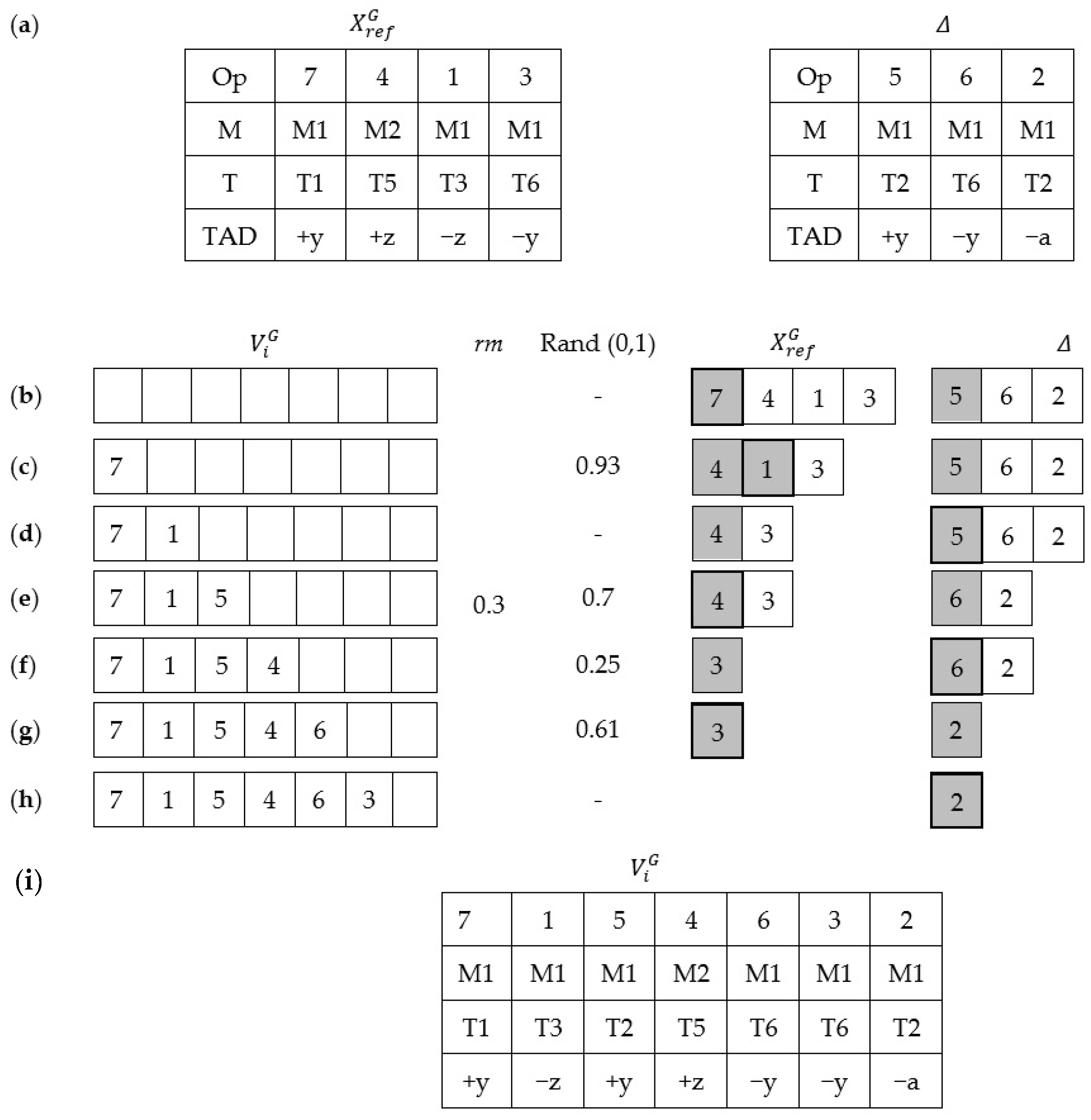
3.5. Discrete Crossover (DC)

The discrete crossover operator generates a trial solution ${\mathrm{U}}_i^G$ by combining the target solution ${\mathrm{X}}_i^G$ and its mutant solution ${\mathrm{V}}_i^G$. This scheme is inspired by the exponential crossover exposed in [40]. The crossover probability $C_r\in \left[\mathrm{0,1}\right]$ indicates which operation will change its resources to minimize the costs generated by the change of machines, tools, and setup (see Figure 4).

Step 1: 

Assign ${\mathrm{V}}_i^G$ to ${\mathrm{U}}_i^G$.

Step 2: 

Select the first column $(j=1)$ in ${\mathrm{U}}_i^G$.

Step 3: 

While $rand\left(\mathrm{0,1}\right)\le C_r$ and $j\le D$ do,

• If the machine ID of the operation ${\mathrm{U}}_i^G\left(j\right)$ could find the candidate machines in the operation ${\mathrm{U}}_i^G(j+1)$; then, the machine ID of the operation ${\mathrm{U}}_i^G(j+1)$ will be the machine ID in ${\mathrm{U}}_i^G\left(j\right)$.
• If the TAD ID of the operation ${\mathrm{U}}_i^G\left(j\right)$ could find the candidate TAD in the operation ${\mathrm{U}}_i^G(j+1)$, then, the TAD ID of the operation ${\mathrm{U}}_i^G(j+1)$ will be the TAD ID in ${\mathrm{U}}_i^G\left(j\right)$, else, select a TAD randomly from the candidate TADs.
• If the tool ID of the operation ${\mathrm{U}}_i^G\left(j\right)$ could find the candidate tools in the operation ${\mathrm{U}}_i^G(j+1)$, then the tool ID in the operation ${\mathrm{U}}_i^G(j+1)$ will be the tool ID in ${\mathrm{U}}_i^G\left(j\right)$.

  $$j=j+1$$

Step 4: 

If $rand\left(\mathrm{0,1}\right){>C}_r$ and $j\le D$, then the missing operations are assigned from ${\mathrm{X}}_i^G$; output ${\mathrm{U}}_i^G$.

Figure 4. Crossover operator: (a) Shows the target ${\mathrm{X}}_i^G$ and mutant solution ${\mathrm{V}}_i^G$; (b) by taking the ${\mathrm{V}}_{\mathrm{i}}^{\mathrm{G}}$ solution as base the operation 7 (j = 1) is the first in the sequence. From this operation on the right-hand side, the resources of operations 3 and 1 are changed if they are available in its list of machines, tools, and TAD. From the operation 5 (j = 4) the condition is not met; therefore, the resources of operations 5, 4, 2, and 6 are obtained from the target solution ${\mathrm{X}}_i^G$.

Figure 4. Crossover operator: (a) Shows the target ${\mathrm{X}}_i^G$ and mutant solution ${\mathrm{V}}_i^G$; (b) by taking the ${\mathrm{V}}_{\mathrm{i}}^{\mathrm{G}}$ solution as base the operation 7 (j = 1) is the first in the sequence. From this operation on the right-hand side, the resources of operations 3 and 1 are changed if they are available in its list of machines, tools, and TAD. From the operation 5 (j = 4) the condition is not met; therefore, the resources of operations 5, 4, 2, and 6 are obtained from the target solution ${\mathrm{X}}_i^G$.

3.6. Selection

The selection is carried out by Equation (14), under the greedy selection or elitist criterion in the same way as the continuous DEA [41]. The trial solution ${\mathrm{U}}_i^G$ is compared with its target solution ${\mathrm{X}}_i^G$, with the lowest total production cost (TC) value, will pass on to the next generation.

$${\mathrm{X}}_i^{G+1}=\left\{\begin{array}{c}{\mathrm{U}}_i^G,\mathrm{si}\mathrm{TC}\left({\mathrm{U}}_i^G\right)\le \mathrm{TC}\left({\mathrm{X}}_i^G\right)\\ {\mathrm{X}}_i^G,\mathrm{otherwise}\end{array}\right..$$

(14)

3.7. Local Search Strategy

The proposed local search strategy aims to improve the local search of the DDEA; it is applied from the $\alpha$ generation every $\mu$ generation and tries to enhance $\beta$ times to the best solution of the updated population ${\mathrm{X}}_{best}^{G+1}$. In this strategy, a column $u$ is selected randomly; it is inserted in a position $k$ along the sequence. If the movement is valid, the ID of the machines, cutting tools and TAD of the operation $u$ are changed by the operations next to them ($k-1$ and $k+1$). The procedure of the local search strategy is described as follows, and an example can be seen in Figure 5:

Step 1: 

Assign ${\mathrm{X}}_{best}^{G+1}$ to ${\mathrm{X}}_{\mathrm{a}\mathrm{u}\mathrm{x}\_\mathrm{b}}$; Set $i=1$.

Step 2: 

While $i\le \beta$

Step 3: 

Select a column $u$ randomly in the ${\mathrm{X}}_{\mathrm{a}\mathrm{u}\mathrm{x}\_\mathrm{b}}$.

Step 4: 

Select randomly a position $k$ between $u$ and $D$.

Step 5: 

Insert the column $u$ in position $k$.

Step 6: 

If the movement of $u$ generates a valid OS, then

Step 6.1: 

To verify the operations machine ID of column $u$,

If the operation of $u$ could be developed for the machine ID of the operation ${\mathrm{X}}_{{\mathrm{a}\mathrm{u}\mathrm{x}}_{\mathrm{b}}}\left(k-1\right),$ it will be changed in column $u$,

Elseif the operation of $u$ could be developed for the machine ID of the operation ${\mathrm{X}}_{{\mathrm{a}\mathrm{u}\mathrm{x}}_{\mathrm{b}}}(k+1)$ it will be changed in column $u$. If the operation machine ID could be changed for both, one is selected randomly; when there is no possibility of change, the current machine ID is kept.

Step 6.2: 

Do the same procedure in 6.1 for Tool ID and TAD ID.

Step 6.3: 

Compare the TC value; if the TC value of ${\mathrm{X}}_{\mathrm{a}\mathrm{u}\mathrm{x}\_\mathrm{b}}<{\mathrm{X}}_{best}^{G+1}$, then assign ${\mathrm{X}}_{\mathrm{a}\mathrm{u}\mathrm{x}\_\mathrm{b}}$ to ${\mathrm{X}}_{best}^{G+1}$.

Step 7: 

$i=i+1$. Go back to step 2.

Step 8: 

output ${\mathrm{X}}_{best}^{G+1}$.

Figure 5. Local search strategy: (a) the $u$ and $k$ columns are selected from ${\mathrm{X}}_{aux\_b}$; (b) once the OS is valid, the machine ID of $u$ could be changed for the machine ID of operations 5 and 2; therefore, the new machine ID of operation 3 is M3. In the tool ID, there is no possibility of change; hence, the tool ID is kept. The TAD ID −z and −a could be selected as new TAD ID; in this case, one is chosen randomly.

Figure 5. Local search strategy: (a) the $u$ and $k$ columns are selected from ${\mathrm{X}}_{aux\_b}$; (b) once the OS is valid, the machine ID of $u$ could be changed for the machine ID of operations 5 and 2; therefore, the new machine ID of operation 3 is M3. In the tool ID, there is no possibility of change; hence, the tool ID is kept. The TAD ID −z and −a could be selected as new TAD ID; in this case, one is chosen randomly.

4. Time Complexity

The time complexity of the DDEA is calculated by adding the time complexities of each stage as follows:

▪

Population initialization, the time complexity of generating a feasible sequence for $NP$ solutions, $t_1=O(NP\times D^2)$.

▪

The complexity of population evaluation, in every individual of population $NP$; the $\mathrm{N}\mathrm{M}\mathrm{C}$, $\mathrm{N}\mathrm{T}\mathrm{C},$ and $\mathrm{N}\mathrm{S}\mathrm{C}$ are calculated, $t_2=O\left(NP\times D\right)$.

▪

The complexity of discrete mutation (MC), in each generation $\left(G\right)$ for every solution in $NP$, a feasible mutant solution is generated where the verification has time complexity $D^2$, $t_3=O\left(G_{max}\times NP\times D^3\right).$

▪

Discrete crossover (DC), $t_4=O(G_{max}\times NP\times D)$.

▪

Selection, $t_5=O(NP\times G_{max})$.

▪

Local search strategy, $t_6=O(G_{max}\times \beta \times D^2)$.

Figure 6 shows the pseudocode of the DDEA.

According to the previous times, the time complexity of the DDEA is $T=t_1+t_2+t_3+t_4+t_5+t_6=O(G_{max}\times NP\times D^3)$. The time complexity of this discrete approach depends on the values of the population number $NP$, the maximum number of generations $G_{max}$, and the number of operations $D$. Therefore, it is essential to tune $NP$ and $G_{max}$ properly to avoid the time increases, mainly due to large operations.

5. Determination of DDEA Parameters

For the DDEA to consistently achieve the minimum costs, it is necessary to tune the number of populations $NP$, the maximum number of generation $G_{max}$, the mutant factor $\mathsf{{\rm Y}}$, assignment probability $rm$, crossover probability $C_r$, the number of generations $\alpha$, $\mu$ and the number of attempts $\beta$ to improve the ${\mathrm{X}}_{best}^{G+1}$. The $NP$ parameters and $G_{max}$ are highly relevant because the execution time depends mainly on them. If these values are too large, the execution time increases; on the other hand, if $NP$ is small, randomness in the candidate solutions is lost, causing them to fall into local minima quickly. If the value of $G_{max}$ is small, the search is interrupted, and if the value is high, more solutions can be explored at the cost of computational time.

However, the $\mathsf{{\rm Y}}$, $rm$, and $C_r$ parameters also influence the quality of the solution. To analyse the performance of each of these parameters without the local search strategy, part 2 ANC-101 obtained from [2] was taken to show the performance and the second case study. To analyse the influence of $\mathsf{{\rm Y}}$, $NP=500$, $G_{max}=250$, $rm=0.85$, $C_r=0.7,$ and $\mathsf{{\rm Y}}$ take values of 0.1, 0.5, and 0.9. Figure 7a shows the three DDEA runs whose minimum TC values are 2544, 2530, and 2560. Only $\mathsf{{\rm Y}}=0.5$ reaches the minimum value at 157, whereas $\mathsf{{\rm Y}}=0.1$ and $0.9$ reach their values in 116 and 126 generations, respectively. Similarly, the parameter $rm$ is analysed, the $NP$ values are kept, $G_{max}$, $\mathsf{{\rm Y}}=0.3$ $C_r=0.7$, and $rm$ takes values of 0.1, 0.5, and 0.9. Figure 7b shows that none of the values assigned to $rm$ reaches the TC values 2547, 2542, and 2535, respectively these values were achieved in 49, 69, and 203 generations, respectively. To show the influence of $C_r$, the $G_{max}$ and $NP$ parameters are kept, then, $\mathsf{{\rm Y}}=0.3$ $rm=0.85$, and $C_r$ take values of 0.1, 0.5, and 0.9. Figure 7c shows that only $C_r=0.9$ reaches the minimum value of 3310 at 104 generations, whereas $C_r=0.5$ and 0.1 reach values noticeably smaller than 2567 and 2560 (16), respectively. The values were achieved in 173 and 16 generations, respectively.

Twenty runs were performed independently to show the influence of the local search strategy. In the first five runs, the local search strategy was not invoked; in the second five, the parameters are set to $\alpha =50$ and $\mu =15$; the subsequent five runs have the parameters $\alpha =100$ and $\mu =10$ and, the last five, $\alpha =150$ and $\mu =5$. All runs were performed with $G_{max}=200$, $NP=500$, $\mathsf{{\rm Y}}=0.1$, $rm=0.85$, $C_r=0.8,$ and $\beta =100$. After these runs, the following was observed: first, when the local search strategy was not invoked, the mean value was 2538.2; furthermore, when it was invoked in all three next cases, the mean value was less than 2538.2. In the first sample, when $\alpha =50$ and $\mu =15$, the mean value was 2532.6; in the second sample, the mean value was 2534.0; in the last sample, the mean value was 2535.2.

It is observed that the DDEA presents better performance with a $\mathsf{{\rm Y}}$ value between 0.1–0.5. This means that to generate the ${\mathrm{V}}_i^G$ solution, the base solution $({\mathrm{X}}_{base}^G$) will be a solution chosen at random $({\mathrm{X}}_{r1}^G$) most of the time, instead of the best of the current population $({\mathrm{X}}_{best}^G$); promoting the exploration of new solutions. The $rm$ value achieves the closest values to minimum TC when the value is found between 0.5–1; the $\mathsf{\Delta }$ operations will be chosen in the creation of the ${\mathrm{V}}_i^G$ solution. With the $C_r$ parameter between 0.5–0.9, the slow convergence is avoided, with small values of $C_r$, machines, tools, and TAD of trial solution ${\mathrm{U}}_i^G$ homogenise more slowly. The local search strategy improves the quality of the solution when it is invoked by around half of all generations.

These parameters were tuned by hand, and several experiments were performed in each part of the case studies, ensuring a good balance between CPU time and efficiency.

Table 1. Parameters used in each case study.

	Part 1	Part 2			Part 3	Part 4				Part 5
	Case 1	Case 1			Case 1	Case 1		Case 2		Case 1
	Cond. 1	Cond. 1	Cond. 2	Cond. 3	Cond. 1	Cond. 1	Cond. 2	Cond. 1	Cond. 2	Cond. 1
$NP$	120	400	300	500	90	500	500	500	500	600
$G_{max}$	120	100	100	100	110	400	400	400	400	450
$\mathsf{{\rm Y}}$	0.001	0.001	0.001	0.01	0.001	0.01	0.01	0.01	0.01	0.001
$rm$	0.5	0.85	0.75	0.1	0.99	0.9	0.9	0.9	0.9	0.9
$C_r$	0.95	0.9	0.9	0.7	0.85	0.9	0.9	0.9	0.9	0.9
$\alpha$	60	50	50	50	60	50	100	250	100	200
$\beta$	20	50	10	40	20	50	20	50	30	50
$\mu$	50	10	10	10	30	20	20	50	60	30

shows the tuned values in the rows, and the part number, case studies, and conditions are indicated in the columns.

6. Case Studies and Results Analysis

To validate the performance, effectiveness, and feasibility of DDEA, five prismatic parts of different complexity from various authors were adopted as case studies: Zhang et al. [12], Hu et al. [19], Huang et al. [28], and Luo et al. [27]. The first three parts have been studied extensively; the other two are the newest and most complex. The DDEA was programmed in MATLAB^® 2022b and executed in Windows 10 Operating System with a core i7 3.60 GHz processor and 32 GB in memory.

To the author’s knowledge, the performance of the cited algorithms has been measured by using the mean, minimum, and maximum values of the total production cost.

Table 2. Results comparison of the analysed cases.

		Condition 1			Condition 2			Condition 3
Algorithm	References	Minimum	Maximum	Mean	Minimum	Maximum	Mean	Minimum	Maximum	Mean
Part 1
ICA	[21]	1739	1749	1741
FSDPSO	[8]	1739	-	1740.7
DDEA		1739	1759	1739.3
Part 2
ACO	[19]	2530		2667	2090		2115
ESGA	[2]	2530	2562	2539.1	2090			2590
FSDPSO	[8]	2530		2532.5	2090		2090
CPAGA	[3]	2530	2535	2530.5	2090	2090	2090	2500	2500	2500
PR-GA	[6]	2530		2530.5	2090		2090
DDEA		2530	2537	2531.1	2090	2120	2096	2590	2600	2594.5
GA-SA	[23]	2527			2120			2590
TS	[11]	2527	2690	2609.6	2120	2390	2208	2580	2740	2630
HBMO	[22]	2525	2557	2543.5	2090	2120	2098	2590	2600	2592
PSO	[18]	2525	2535	2527.2	2090	2120	2093.0	2590	2600	2593.2
HGGA	[26]	2527	2585		2120			2590
ACO	[4]	2525	2557	2552.4	2090	2380	2120.5	2590	2740	2600.8
PR-GA	[6]	2525		2525	2090		2090
DDEA		2525	2532	2526.5	2090	2120	2096	2590	2600	2594
Part 3
PSO	[5]	1361		1430
GA	[5]	1381		1447.4
SA	[5]	1421		1447.4
ICA	[21]	1357		1364.1
ACO	[19]	1357		1419
FSDPSO	[8]	1357		1359
PR-GA	[6]	1357		1357
DDEA		1357	1357	1357
Part 4
Case 1
GA-SA	[28]	4368	-	-	4450	-	-
DDEA		4206	4635	4373.2	4310	4805	4492.7
Part 4
Case 2
CPAGA	[3]	4299	4315	4302	4503	4503	-
PR-GA	[6]	4098		4232.8	4151		4298.4
DDEA		4098	4524	4271.1	4151	4530	4324.9
Part 5
Standard GA	[27]	29.7		29.31
Hybrid GA	[27]	27.3		27.82
DDEA		23.9	26.7	25.51

shows the part number set, the used algorithms, and the case number. The columns show the algorithm name and reference, respectively. The authors used different numbers of runs, cases, and conditions depending on the part. For example, parts 1, 3, and 5 have one case study, part 2 has three conditions, and part 4 contains two cases, each with two conditions. Additionally, Section 6.6 describes a statistical analysis based on quantiles.

6.1. Part 1

Part 1 is taken from [12], which has 19 features and 23 operations. For this part, the DDEA was executed 60 times with the parameters listed in Table 1 column “Part 1”, under the following conditions: All machines and tools are available, and ${\omega }_1-{\omega }_5=1$, this means that all machining and setup costs are considered. The SCC is calculated according to [9,12]. The DDEA results are compared with the ICA methods presented in [21] and FSDPSO in [8] (see Table 2); the mean value obtained exceeds both approaches.

6.2. Part 2

Part 2 is the ANC-101, taken from [2]; it is one of the most studied parts in the literature, with 14 features and 20 operations. To test the proposed approach, three conditions are taken: (1) all the machines and cutting tools are available, and ${\omega }_1-{\omega }_5=1$; (2) all machines and tools are available without considering the cost involved in tools and their changes; therefore, ${\omega }_2={\omega }_4=0$ and ${\omega }_1={\omega }_3={\omega }_5=1$; (3) machine M2 and tool T7 are not available and, ${\omega }_2={\omega }_4=0$ and ${\omega }_1={\omega }_3={\omega }_5=1$. The DDEA executed 20 runs with the column “Part 2” parameters in Table 1; it was compared with the different approaches. Two cases were performed; the first did not include the T6 in Op6, and the second did. The algorithms that operate the first case were ACO [19], ESGA [2], FSDPSO [8], CPAGA by [3], and PR-GA [6]. Under conditions (1) and (2), the TC value is similar to the reported values, whereas for case (3), the DDEA and ESGA [2] achieve a TC = 2590 and a mean of 2594.5 (see Table 2). For this case, the approach CPAGA presented in [3] obtained a sequence with TC = 2500, shown in Table 12 of that research. However, the sequence is not feasible because Op12 must be performed before Op19 and Op20 according to their constraints (Table 6 of [3]). For the second case, the approaches GA-SA [23], TS [11], HBMO [22], PSO [18], HGGA [26], ACO [4], and PR-GA [6] were considered. With this change, the TC values in condition (1) are slightly less.

6.3. Part 3

Part 3 was selected from [19] with 11 features and 14 operations. In this case, all the machines and tools are available. The DDEA was executed 20 times with the parameters listed in column “Part 3” in Table 1. The results were compared with the approaches reported by Guo et al. in [5], ICA [21], ACO [19], FSDPSO [8] and PR-GA [6] see Table 2. The DDEA obtained the best value of TC (1357), as reported by the ACO, FSDPSO, and PR-GA approaches, and the PR-GA obtained the same mean value.

6.4. Part 4

Part 4, taken from [28], is one of the most complex parts. It has 28 features and 46 operations. For this part, two conditions were considered. In condition (1), all machines and cutting tools are available and ${\omega }_1-{\omega }_5=1,$ and for condition (2), the machines M03, M07, and tool T08 are not available and ${\omega }_1-{\omega }_5=1$. The DDEA was executed 20 times in each condition with the parameters listed in column “Part 4” in Table 1. In the first case, the M6 machine was assigned for operations Op17 to Op20, remaining as candidate machines M3, M4, M6, and M7. The DDEA approach was compared with GA-SA [28]. The plan obtained under condition 1 has a TC value of 4206, better than the plan presented by GA-SA. It should be highlighted that the plan obtained by the hybrid approach is infeasible since Op8 must be performed after Op30, Op31, and Op32; this can be corroborated in the OPG of Figure 8 of the mentioned research; moreover, machine M3 is assigned to Op12, which is not available for this operation (only M4 and M5 can be used). Similarly, for condition 2, the DDEA achieved a plan with a lower TC (4310) value. For this reason, the best sequences obtained by DDEA for case 1 of part 4 are shown in

Table 3. The best sequence obtained by DDEA for part 4 in case 1.

Case (1), Condition (1)
Order	1	2	3	4	5	6	7	8	9	10	11	12	13	14	15	16	17	18	19	20	21	22	23
Op	1	10	13	11	14	22	9	2	3	24	25	27	26	28	34	35	36	37	45	46	4	5	6
M	1	5	5	5	5	5	5	2	2	9	9	9	9	9	7	7	7	7	7	7	7	7	7
T	1	8	8	8	8	8	8	1	1	11	22	13	12	14	28	24	17	25	19	27	4	5	5
TAD	+z	−z	−z	−z	−z	−z	+z	+z	+z	+z	+z	+z	+z	+z	−c	−c	−c	−c	−x	−x	−y	−y	−y
Continued	24	25	26	27	28	29	30	31	32	33	34	35	36	37	38	39	40	41	42	43	44	45	46
Op cont.	29	30	17	19	20	18	7	31	32	33	8	15	16	12	41	39	40	42	23	38	21	43	44
M cont.	7	7	7	7	7	7	7	7	7	7	4	4	4	4	9	9	9	9	9	9	9	9	9
T cont.	6	6	7	7	7	7	7	15	16	23	8	8	8	8	18	18	26	26	20	21	10	18	26
TAD cont.	−y	−y	−b	−b	−b	−b	−a	−a	−a	−a	−a	−z	−z	−z	−b	−b	−b	−b	−z	−z	−z	−z	−z
TMC = 1529	TTC = 277			MCC = 720			TCC = 420			SCC = 1260			TC = 4206
Case (1), Condition (2)
Order	1	2	3	4	5	6	7	8	9	10	11	12	13	14	15	16	17	18	19	20	21	22	23
Op	1	11	13	14	10	22	9	2	3	26	27	24	25	28	45	46	34	35	36	37	29	30	4
M	1	5	5	5	5	5	5	2	2	9	9	9	9	9	8	8	8	8	8	8	8	8	8
T	1	9	9	9	9	9	9	1	1	12	13	11	22	14	19	27	28	24	17	25	6	6	4
TAD	+z	−z	−z	−z	−z	−z	+z	+z	+z	+z	+z	+z	+z	+z	−x	−x	−c	−c	−c	−c	−y	−y	−y
Continued	24	25	26	27	28	29	30	31	32	33	34	35	36	37	38	39	40	41	42	43	44	45	46
Op cont.	5	6	7	31	32	33	8	17	18	19	20	15	16	12	21	43	44	23	38	39	41	40	42
M cont.	8	8	8	8	8	8	4	4	4	4	4	4	4	4	9	9	9	9	9	9	9	9	9
T cont.	5	5	7	15	16	23	7	7	7	7	7	7	7	9	10	18	26	20	21	18	18	26	26
TAD cont.	−y	−y	−a	−a	−a	−a	−a	−b	−b	−b	−b	−z	−z	−z	−z	−z	−z	−z	−z	−b	−b	−b	−b
TMC = 1614	TTC = 281			MCC = 720			TCC = 435			SCC = 1260			TC = 4310

TMC: Total machine cost; TTC: Total tool cost; MCC: Machine change cost; TCC: Tool change cost; SCC: Setup change cost; TC: Total cost.

.

In the second case, the DDEA approach was compared with the approaches CPAGA [3] and PR-GA [6]. For this comparison, the machine M5 was assigned instead of M6 for operations Op17 to Op20, remaining as candidate machines M3, M4, M5, and M7. The results are shown in Table 2; for both conditions, the DDEA approach obtained the minimum TC (4098 and 4151) value.

6.5. Part 5

Part 5 is a real-world problem from [27] with 42 features and 76 operations. For this part, the DDEA approach was executed 10 times with the parameters listed in column “Part 5” in Table 1. For this case, the TC is computed considering the setup cost by using Equation 18, where $f_1\left(x\right)$ is the total number of machine changes (Equation (15)), $f_2\left(x\right)$ represents the total number of tool changes (Equation (16)) and $f_3\left(x\right)$ is the total number of TAD changes (Equation (17)). To compare the DDEA with the standard and hybrid GA approaches, the $\mathsf{\theta }$, $\mathsf{\lambda }$ and $\mathsf{\tau }$ weight values are set to 0.45, 0.25, and 0.3, respectively, according to [27].

$$f_1(x)={\sum }_{i=1}^{D-1}\left({\mathsf{\Omega }}_1({\mathrm{M}}_{i+1},{\mathrm{M}}_i)\right),$$

(15)

$$f_2(x)={\sum }_{i=1}^{D-1}\left({\mathsf{\Omega }}_1({\mathrm{T}}_{i+1},{\mathrm{T}}_i)\right),$$

(16)

$$f_3(x)={\sum }_{i=1}^{D-1}{\mathsf{\Omega }}_2\left({\mathsf{\Omega }}_1({\mathrm{M}}_{i+1},{\mathrm{M}}_i),{\mathsf{\Omega }}_1({\mathrm{T}\mathrm{A}\mathrm{D}}_{i+1},{\mathrm{T}\mathrm{A}\mathrm{D}}_i)\right),$$

(17)

$$\mathrm{T}\mathrm{C}=\mathsf{\theta }{f}_1\left(x\right)+\mathsf{\lambda }{f}_2\left(x\right)+\mathsf{\tau }{f}_3\left(x\right).$$

(18)

The DDEA improves the minimum TC (23.9) and the mean cost (25.51). For this reason, the best plan obtained is shown in

Table 4. The best sequence obtained by DDEA for part 5.

Order	1	2	3	4	5	6	7	8	9	10	11	12	13	14	15	16	17	18	19	20	21	22	23
Op	66	18	47	71	35	5	10	11	7	8	9	12	62	63	39	40	30	33	34	75	76	1	2
M	1	1	1	1	1	1	1	1	1	1	1	1	1	2	2	2	2	2	2	2	2	2	2
T	6	6	6	6	6	6	9	26	7	8	25	10	23	34	1	1	1	1	1	1	1	1	2
TAD	E	B	D	F	C	A	A	A	A	A	A	A	E	E	D	D	C	C	C	F	F	A	A
Continued	24	25	26	27	28	29	30	31	32	33	34	35	36	37	38	39	40	41	42	43	44	45	46
Op cont.	3	69	70	73	74	72	6	37	27	28	29	36	24	25	26	43	38	41	44	49	50	42	48
M cont.	2	1	1	1	1	1	1	1	1	1	1	1	1	1	1	1	1	1	1	1	1	1	1
T cont.	3	13	28	24	31	5	5	17	16	39	29	5	12	27	36	37	18	19	20	13	28	30	5
TAD cont.	A	F	F	F	F	F	A	C	C	C	C	C	C	C	C	D	D	D	D	D	D	D	D
Continued	47	48	49	50	51	52	53	54	55	56	57	58	59	60	61	62	63	64	65	66	67	68	69
Op cont.	64	60	61	54	55	53	56	51	52	65	67	68	57	58	13	31	32	45	46	59	14	20	23
M cont.	1	1	1	1	1	1	1	1	1	1	1	1	1	2	2	2	2	2	2	1	1	1	1
T cont.	41	8	25	19	30	21	35	12	27	37	6	6	22	33	32	2	3	3	3	40	38	13	15
TAD cont.	E	E	E	E	E	E	E	E	E	E	E	E	E	E	B	C	C	D	D	E	B	B	B
Continued	70	71	72	73	74	75	76
Op cont.	15	16	17	21	22	19	4
M cont.	1	1	1	1	1	1	3
T cont.	11	12	27	28	14	5	4
TAD cont.	B	B	B	B	B	B	A
TMC = 0	TTC = 0			MCC = 5			TCC = 59			SCC = 23			TC = 23.9

TMC: Total machine cost; TTC: Total tool cost; MCC: Machine change cost; TCC: Tool change cost; SCC: Setup change cost; TC: Total cost.

. It presents 5 machine changes, 59 tool changes and 23 setup changes, which show an improvement compared with the plan obtained by hybrid GA because the hybrid GA plan presents 15 machine changes, 69 tool changes, and 19 setup changes. Figure 8 shows the DDEA convergence in the iteration number (109) between the best and worst run, which is faster than the standard GA and Hybrid GA, around 350 and 400 iterations, respectively (Figure 8 of [27]). The plans obtained for standard GA and Hybrid GA approaches have incorrect assignments of machines and tools in several operations, according to Table 1 of [27]. For example, in the plan obtained by the hybrid algorithm, the Op22 is performed by machine M02 and tool T15, but this operation can only be performed by machine M01 and tool T14. Likewise, the plan obtained by the standard GA, the Op33, is performed by M03 and can only be performed by M02.

6.6. Statistical Analysis to Performance Measure

To complement the performance measures of the DDEA (arithmetic mean and best solution found), an approach based on quantiles purposes by Nikola et al. [42] was added, which makes it possible to consider the distribution of the data and to specify the solution quality and the probability of reaching. The quantile $Q_p$ is associated with a probability $p,$ therefore, if the quality solution for some algorithm is known, then the probability of achieving a solution that is equal to or better than $Q_p$ is greater than or equal to $p$. For example, for part 2 of condition 1, the best solution is in $Q_{0.5}=2530$, at least a 0.5 probability of getting a solution with a quality equal to 2530 or better.

Table 5. Quantiles of each part.

	Part 1	Part 2			Part 3	Part 4				Part 5
	Case 1	Case 1			Case 1	Case 1		Case 2		Case 1
	Cond. 1	Cond. 1	Cond. 2	Cond. 3	Cond. 1	Cond. 1	Cond. 2	Cond. 1	Cond. 2	Cond. 1
$Q_{0.1}$	1739	2530	2090	2590	1357	4231.5	4313.9	4134	4200	23.96
$Q_{0.2}$	1739	2530	2090	2590	1357	4258.2	4433	4134	4200	24.66
$Q_{0.5}$	1739	2530	2090	2590	1357	4365	4460	4254	4321	25.37
$Q_{0.8}$	1739	2532	2090	2600	1357	4451	4592	4368.8	4425	26.43
$Q_{0.9}$	1739	2535	2120	2600	1357	4568.9	4661.6	4474.8	4509	26.67

shows the quantiles of every part; for part 3, the proposed approach always found the best solution, which means it has a probability equal to 1 of finding the best solution. For part 1, the best solution has a quality $Q_{0.9}$ which means there is at least a 0.9 probability of obtaining a solution with a quality equal to 1739; finding this kind of solution requires at least one execution. For part 2, in cases 1 and 3, the probability of obtaining the best solution is 0.5; condition 2 is slightly higher (0.8). For all conditions in parts 4 and 5, the quality of the best solution is smaller than $Q_{0.1}$ to obtain these values again more runs are needed.

6.7. Computing Time for the Approaches

Recent studies have considered CPU processing time; however, it is a relative measure that depends on many factors, such as the capabilities of the computer equipment, programming language, and coding best practices, among other factors.

Table 6. CPU time of some approaches in seconds.

		Part 1	Part 2			Part 3	Part 4				Part 5
		Case 1	Case 1			Case 1	Case 1		Case 2		Case 1
Algorithm	References	Cond. 1	Cond. 1	Cond. 2	Cond. 3	Cond. 1	Cond. 1	Cond. 2	Cond. 1	Cond. 2	Cond. 1
ESGA	[2]	-	5.07	-	-	-	-	-			-
TSGA	[2]	-	4.91	-	-	-	-	-			-
FSDPSO	[8]	-	0.727	0.742	-	0.427	-	-			-
CPAGA	[3]	-	1.94	1.24	1.3	-	3.26	-			-
PR-GA	[6]	-	1.10	0.46	-	2.08	9.605	-			-
DDEA		4.274	6.164	4.614	8.687	1.317	61.865	65.559	61.167	59.125	141.167

shows the average time results of the DDEA and the approaches that have considered this parameter (ESGA, FSDPSO, CPAGA, and PR-GA). The authors in [3] consider the time of the best results instead of the average time. The DDEA approach obtains the minimum TC values for each part and good computing times. The elapsed times for parts 1 and 4 in conditions 2 and 5 were 4.274 s, 59.120 s, and 141.167 s, respectively. Despite the times obtained by DDEA, these could be about ten times faster if programmed in C/C++ language [43,44].

7. Conclusions and Future Work

This work implemented a novel Discrete Differential Evolution Algorithm to solve the OS problem in the CAPP system; it performs the search in the feasible solution space using an integer representation. The Discrete Mutation promotes the search for new solutions and reduces the machining cost, while the Discrete Crossover reduces the setup cost. The Selection stage ensures that the best candidate goes to the next generation; finally, the local search strategy tries to improve the best solution by moving an operation and changing its adjacent resources. A statistical approach based on quantiles was implemented, and this shows that the DDEA has good performance for parts with a small number of machining operations, and the probability of achieving it is high; for parts with a high number of machining operations, the performance is good, but the likelihood of archiving it requires more runs. Five parts, with different features and restrictions, were selected from the literature to prove its efficiency and effectiveness. As a result, the DDEA obtained better TC values for part 4 and part 5 in comparison with the GA algorithms [27,28]. Part 1 obtained a better mean value than ICA and FSDPSO; part 3 received the same value from the PR-GA approach.

The DDEA requires an automatic parameter tuning stage because the process is performed by hand. The idea is to implement an algorithm to reduce the search space of feasible solutions to obtain a high probability of achieving the solution in fewer runs to improve the manufacturing cycle. In the future, we will extend the application of DDEA to upstream and downstream stages, such as automatic feature recognition and scheduling problems.

References

- Wu, W.; Huang, Z.; Wu, K.; Chen, Y. An optimization approach for setup planning and operation sequencing with tolerance constraints. Int. J. Adv. Manuf. Technol. 2020, 106, 4965–4985. [Google Scholar] [CrossRef]
- Su, Y.; Chu, X.; Chen, D.; Sun, X. A genetic algorithm for operation sequencing in CAPP using edge selection based encoding strategy. J. Intell. Manuf. 2018, 29, 313–332. [Google Scholar] [CrossRef]
- Falih, A.; Shammari, A.Z.M. Hybrid constrained permutation algorithm and genetic algorithm for process planning problem. J. Intell. Manuf. 2020, 31, 1079–1099. [Google Scholar] [CrossRef]
- Wang, J.F.; Wu, X.; Fan, X. A two-stage ant colony optimization approach based on a directed graph for process planning. Int. J. Adv. Manuf. Technol. 2015, 80, 839–850. [Google Scholar] [CrossRef]
- Guo, Y.W.; Mileham, A.R.; Owen, G.W.; Li, W.D. Operation sequencing optimization using a particle swarm optimization approach. Proc. Inst. Mech. Eng. B J. Eng. Manuf. 2006, 220, 1945–1958. [Google Scholar] [CrossRef]
- Dou, J.; Wang, S.; Zhang, C.; Shi, Y. A genetic algorithm with path-relinking for operation sequencing in CAPP. Int. J. Adv. Manuf. Technol. 2023, 125, 3667–3690. [Google Scholar] [CrossRef]
- Liu, X.J.; Yi, H.; Ni, Z.H. Application of ant colony optimization algorithm in process planning optimization. J. Intell. Manuf. 2013, 24, 1–13. [Google Scholar] [CrossRef]
- Dou, J.; Li, J.; Su, C. A discrete particle swarm optimisation for operation sequencing in CAPP. Int. J. Prod. Res. 2018, 56, 3795–3814. [Google Scholar] [CrossRef]
- Ma, G.H.; Zhang, Y.F.; Nee, A.Y.C. A simulated annealing-based optimization algorithm for process planning. Int. J. Prod. Res. 2000, 38, 2671–2687. [Google Scholar] [CrossRef]
- Nallakumarasamy, G.; Srinivasan, P.S.S.; Raja, K.V.; Malayalamurthi, R. Optimization of operation sequencing in CAPP using simulated annealing technique (SAT). Int. J. Adv. Manuf. Technol. 2011, 54, 721–728. [Google Scholar] [CrossRef]
- Li, W.D.; Ong, S.K.; Nee, A.Y.C. Optimization of process plans using a constraint-based tabu search approach. Int. J. Prod. Res. 2004, 42, 1955–1985. [Google Scholar] [CrossRef]
- Zhang, F.; Zhang, Y.F.; Nee, A.Y.C. Using genetic algorithms in process planning for job shop machining. IEEE Trans. Evol. Comput. 1997, 1, 278–289. [Google Scholar] [CrossRef]
- Salehi, M.; Tavakkoli-Moghaddam, R. Application of genetic algorithm to computer-aided process planning in preliminary and detailed planning. Eng. Appl. Artif. Intell. 2009, 22, 1179–1187. [Google Scholar] [CrossRef]
- Guo, Y.W.; Mileham, A.R.; Owen, G.W.; Maropoulos, P.G.; Li, W.D. Operation sequencing optimization for five-axis prismatic parts using a particle swarm optimization approach. Proc. Inst. Mech. Eng. B J. Eng. Manuf. 2009, 223, 485–497. [Google Scholar] [CrossRef]
- Guo, Y.W.; Li, W.D.; Mileham, A.R.; Owen, G.W. Applications of particle swarm optimisation in integrated process planning and scheduling. Robot. Comput. Integr. Manuf. 2009, 25, 280–288. [Google Scholar] [CrossRef]
- Kafashi, S.; Shakeri, M.; Abedini, V. Automated setup planning in CAPP: A modified particle swarm optimisation-based approach. Int. J. Prod. Res. 2012, 50, 4127–4140. [Google Scholar] [CrossRef]
- Li, X.; Gao, L.; Wen, X. Application of an efficient modified particle swarm optimization algorithm for process planning. Int. J. Adv. Manuf. Technol. 2013, 67, 1355–1369. [Google Scholar] [CrossRef]
- Wang, J.F.; Kang, W.L.; Zhao, J.L.; Chu, K.Y. A simulation approach to the process planning problem using a modified particle swarm optimization. Adv. Prod. Eng. Manag. 2016, 11, 77–92. [Google Scholar] [CrossRef]
- Hu, Q.; Qiao, L.; Peng, G. An ant colony approach to operation sequencing optimization in process planning. Proc. Inst. Mech. Eng. Part B J. Eng. Manuf. 2017, 231, 470–489. [Google Scholar] [CrossRef]
- Wang, J.; Fan, X.; Wan, S. A graph-based ant colony optimization approach for process planning. Sci. World J. 2014, 2014, 271895. [Google Scholar] [CrossRef]
- Lian, K.; Zhang, C.; Shao, X.; Gao, L. Optimization of process planning with various flexibilities using an imperialist competitive algorithm. Int. J. Adv. Manuf. Technol. 2012, 59, 815–828. [Google Scholar] [CrossRef]
- Wen, X.Y.; Li, X.Y.; Gao, L.; Sang, H.Y. Honey bees mating optimization algorithm for process planning problem. J. Intell. Manuf. 2014, 25, 459–472. [Google Scholar] [CrossRef]
- Li, W.D.; Ong, S.K.; Nee, A.Y.C. Hybrid genetic algorithm and simulated annealing approach for the optimization of process plans for prismatic parts. Int. J. Prod. Res. 2002, 40, 1899–1922. [Google Scholar] [CrossRef]
- Li, L.; Fuh, J.Y.H.; Zhang, Y.F.; Nee, A.Y.C. Application of genetic algorithm to computer-aided process planning in distributed manufacturing environments. Robot. Comput. Integr. Manuf. 2005, 21, 568–578. [Google Scholar] [CrossRef]
- Salehi, M.; Bahreininejad, A. Optimization process planning using hybrid genetic algorithm and intelligent search for job shop machining. J. Intell. Manuf. 2011, 22, 643–652. [Google Scholar] [CrossRef]
- Huang, W.; Hu, Y.; Cai, L. An effective hybrid graph and genetic algorithm approach to process planning optimization for prismatic parts. Int. J. Adv. Manuf. Technol. 2012, 62, 1219–1232. [Google Scholar] [CrossRef]
- Luo, Y.; Pan, Y.; Li, C.; Tang, H. A hybrid algorithm combining genetic algorithm and variable neighborhood search for process sequencing optimization of large-size problem. Int. J. Comput. Integr. Manuf. 2020, 33, 962–981. [Google Scholar] [CrossRef]
- Huang, W.; Lin, W.; Xu, S. Application of graph theory and hybrid GA-SA for operation sequencing in a dynamic workshop environment. Comput. Aided Des. Appl. 2017, 14, 148–159. [Google Scholar] [CrossRef]
- Wang, Y.F.; Zhang, Y.F.; Fuh, J.Y.H. A hybrid particle swarm based method for process planning optimisation. Int. J. Prod. Res. 2012, 50, 277–292. [Google Scholar] [CrossRef]
- Kennedy, J.; Eberhart, R. Particle Swarm Optimization. In Proceedings of the ICNN’95—International Conference on Neural Networks, Perth, Australia, 27 November–1 December 1995; Volume 4, pp. 1942–1948. [Google Scholar] [CrossRef]
- Santucci, V.; Baioletti, M.; Milani, A. Algebraic differential evolution algorithm for the permutation flowshop scheduling problem with total flowtime criterion. IEEE Trans. Evol. Comput. 2016, 20, 682–694. [Google Scholar] [CrossRef]
- Storm, R.; Price, K. Differential Evolution—A Simple and Efficient Heuristic for Global Optimization over Continuous Spaces. J. Glob. Optim. 1997, 11, 341–359. [Google Scholar] [CrossRef]
- Zhang, G.; Xing, K.; Cao, F. Discrete differential evolution algorithm for distributed blocking flowshop scheduling with makespan criterion. Eng. Appl. Artif. Intell. 2018, 76, 96–107. [Google Scholar] [CrossRef]
- Piotrowski, A.P.; Piotrowska, A.E. Differential Evolution and Particle Swarm Optimization against COVID-19. Artif. Intell. Rev. 2022, 55, 2149–2219. [Google Scholar] [CrossRef]
- Ali, I.M.; Essam, D.; Kasmarik, K. A novel differential evolution mapping technique for generic combinatorial optimization problems. Appl. Soft Comput. J. 2019, 80, 297–309. [Google Scholar] [CrossRef]
- Ali, I.M.; Essam, D.; Kasmarik, K. A novel design of differential evolution for solving discrete traveling salesman problems. Swarm Evol. Comput. 2020, 52, 100607. [Google Scholar] [CrossRef]
- Onwubolu, G.C.; Davendra, D. Differential Evolution: A Handbook for Global Permutation-Based Combinatorial Optimization; Springer: Berlin/Heidelberg, Germany, 2009; Volume 175. [Google Scholar] [CrossRef]
- Yuan, S.; Li, T.; Wang, B. A discrete differential evolution algorithm for flow shop group scheduling problem with sequence-dependent setup and transportation times. J. Intell. Manuf. 2021, 32, 427–439. [Google Scholar] [CrossRef]
- Yun, Y.; Moon, C. Genetic algorithm approach for precedence-constrained sequencing problems. J. Intell. Manuf. 2011, 22, 379–388. [Google Scholar] [CrossRef]
- Price, K.V.; Storm, R.M.; Laminen, J.A. Differential Evolution A Practical Approach to Global Optimization, 1st ed.; Springer: Berlin/Heidelberg, Germany, 2005. [Google Scholar] [CrossRef]
- Mohamed, A.W.; Sabry, H.Z. Constrained optimization based on modified differential evolution algorithm. Inf. Sci. 2012, 194, 171–208. [Google Scholar] [CrossRef]
- Ivkovic, N.; Jakobovic, D.; Golub, M. Measuring Performance of Optimization Algorithms in Evolutionary Computation. Int. J. Mach. Learn. Comput. 2016, 6, 167–171. [Google Scholar] [CrossRef]
- Yang, X.; Wang, X.; Liu, Z.; Shu, F. M2Coder: A Fully Automated Translator from Matlab M-functions to C/C++ Codes for ACS Motion Controllers. In Advances in Guidance, Navigation and Control; Yan, L., Duan, H., Deng, Y., Eds.; Springer Nature: Singapore, 2023; pp. 3130–3139. [Google Scholar]
- Jiang, R.M.; Bouridane, A.; Amira, A. Color Saliency Evaluation for Video Game Design. In Advances in Low-Level Color Image Processing; Celebi, M.E., Smolka, B., Eds.; Springer: Dordrecht, The Netherlands, 2014; pp. 409–425. [Google Scholar] [CrossRef]