A Block Triple-Relaxation-Time Lattice Boltzmann Method for Solid–Liquid Phase Change Problem

Abstract

This study introduces a block triple-relaxation-time (B-TriRT) lattice Boltzmann model designed specifically for simulating melting phenomena within a rectangular cavity subject to intense heating from below, characterized by high Rayleigh ($Ra$) numbers ($Ra={10}^8$). Through benchmark testing, it is demonstrated that the proposed B-TriRT approach markedly mitigates numerical diffusion along the phase interface. Furthermore, an examination of the heated region’s placement is conducted, revealing its significant impact on the rate of melting. Notably, findings suggest that optimal melting occurs most rapidly when the heated region is positioned centrally within the cavity.

1. Introduction

The study of thermal flow problems involving phase changes holds paramount importance for both academic inquiry and practical engineering applications. Phase change processes entail intricate thermodynamic phenomena, presenting numerous academic challenges. Among these, the solid–liquid phase change problem stands out due to its widespread occurrence in various engineering domains. Applications such as latent heat thermal energy storage [1,2], battery thermal management [3,4], etc., all play significant roles in modern industry [5].

The investigation of melting phenomena within rectangular enclosures has been the subject of numerous analytical, numerical, and experimental inquiries. Notably, Chen et al. [6] devised a solid–liquid phase change model tailored to simulate phase changes within porous media. Chiappini [7] introduced a hybrid LB-FV methodology to address phase change material dynamics and showcased its versatility across various scenarios. Additionally, the thermal characteristics of phase change materials, encompassing solidification and melting processes, were computationally elucidated through a multi-physics solver. Rui et al. [8] explored natural-convection-induced melting within square cavities, developing an enthalpy-based lattice Boltzmann model integrated with the pseudo-potential lattice Boltzmann approach to accurately delineate solid–liquid interfaces. Chen and Shu et al. [9] advanced a phase-field-simplified lattice Boltzmann method specifically tailored for modeling solid–liquid phase transitions within homogeneous materials. This approach adeptly captures intricate geometries and flow dynamics encountered in such systems. Furthermore, Han et al. [10] conducted an investigation into enhancing the melting performance of composite phase change materials reconstructed via the QSGS method. Their study involved a detailed analysis and comparison of melting front evolution and transient temperature responses between composite and pure phase change materials, offering valuable insights into their thermal behavior.

However, investigations into the melting behavior of phase change materials (PCMs) subjected to bottom heating are notably lacking. It is widely recognized that when heated from below, the heat transfer dynamics resemble classical Rayleigh–Bénard convection, potentially inducing turbulent thermal convection at elevated Rayleigh numbers [11]. A comprehensive comprehension of the intricate transport mechanisms within thermal convective flows necessitates robust experimental and computational methodologies. Over the past three decades, the lattice Boltzmann method (LBM) has emerged as a prominent numerical technique and serves as a formidable tool for computational fluid dynamics and heat transfer analyses [12,13,14,15,16,17]. Moreover, LBM offers a potent approach for solving nonlinear partial differential equations [18,19], encompassing the Navier–Stokes equation, convection–diffusion equation [20], phase field equation [21], and Nernst–Planck equation [22], among others [23]. While numerous LBM models have been proposed for solid–liquid phase change phenomena, the single-relaxation-time (SRT) model remains prevalent [24]. Despite its numerical efficiency, the SRT model often exhibits instability in high-Rayleigh-number scenarios and suffers from numerical diffusion across phase interfaces, as highlighted by Huang. Although Huang [25] mitigated this issue using the multiple-relaxation-time (MRT) model, determining the free relaxation parameters proves cumbersome. In the subsequent discourse, Liu et al. [26] introduce a cascaded LBM tailored for investigating solid–liquid phase change heat transfer. Comparative evaluations with the MRT method demonstrate the superior numerical stability of the cascaded lattice Boltzmann method, which is attributed to enhanced Galilean invariance. Additionally, a novel enthalpy-based immersed boundary-lattice Boltzmann model is proposed for addressing solid–liquid phase change challenges within porous media under local thermal non-equilibrium conditions in reference [27]. Notably, recent advancements include the introduction of a simple yet efficient MRT-LBM for modeling anisotropic liquid–solid phase transitions [28].

In this work, we present a block triple-relaxation-time (B-TriRT) model to solve the phase change problem that has fewer relaxation parameters to be determined than the MRT model and can also reduce the numerical diffusion. The rest of this paper is organized as follows. In Section 2, the B-TriRT LBM is developed for the solid–liquid phase change problem. Section 3 presents the numerical diffusion analysis of the B-TriRT LBM for solid–liquid phase transition. Several numerical experiments, including one-phase melting by conduction and melting in a cavity heated locally from below, are carried out in Section 4. At last, some conclusions are summarized in Section 5.

2. The Block Triple-Relaxation-Time Lattice Boltzmann Model

The governing equations of the solid–liquid phase change problem consist of the incompressible Navier–Stokes (N-S) equations and the energy conservation equation, which have the following form:

$$\nabla ·\mathbf{u}=0,$$

(1)

$$\frac{\partial \mathbf{u}}{\partial t}+\nabla ·\mathbf{uu}=-\nabla p+\nabla ·(\nu \nabla \mathbf{u})+\mathbf{F},$$

(2)

$$\frac{\partial H}{\partial t}+\nabla ·\left(C_{p}T\mathbf{u}\right)=\frac{1}{{\rho }_0}\nabla ·(\kappa \nabla T),$$

(3)

where $\mathbf{u},p$ and $\nu$ are the velocity, pressure and kinematic viscosity, respectively. $\mathbf{F}$ is the external force; according to the Boussinesq approximation, it can be given by

$$\mathbf{F}=\mathbf{g}\beta (T-T_{ref}),$$

(4)

where $\mathbf{g}$ is the gravitational acceleration vector, $\beta$ is the thermal expansion coefficient, and T and $T_{ref}$ are the temperature and reference temperature, respectively. $C_p,\kappa ,{\rho }_0$ are the specific heat, thermal conductivity and referenced density, respectively. $H=C_{p}T+f_{l}L$ is the total enthalpy, with $f_l,L$ representing the liquid fraction and latent heat.

To improve the numerical stability of LBM, the B-TriRT LBM [29,30] is employed for the governing Equations (1)–(3). In the B-TriRT model for the incompressible N-S equations, the evolution of the distribution function is given by

$$\begin{array}{cc}\hfill f_i(\mathbf{x}+{\mathbf{c}}_i\Delta t,t+\Delta t)=& f_i(\mathbf{x},t)-{\overline{k}}_0{f}_i^{neq}(\mathbf{x},t)-({\overline{k}}_1-{\overline{k}}_0)\frac{{\omega }_i{\mathbf{c}}_i·{\mathbf{M}}_{f1}^{neq}(\mathbf{x},t)}{c_s^2}\hfill \\ \hfill & -({\overline{k}}_2-{\overline{k}}_0)\frac{{\omega }_i({\mathbf{c}}_i{\mathbf{c}}_i-c_s^2\mathbf{I}):{\mathbf{M}}_{f2}^{neq}(\mathbf{x},t)}{2c_s^4}+(1-\frac{{\overline{k}}_1}{2})\frac{{\omega }_i{\mathbf{c}}_i·\mathbf{F}}{c_s^2}\hfill \\ \hfill & +(1-\frac{{\overline{k}}_2}{2})\frac{{\omega }_i({\mathbf{c}}_i{\mathbf{c}}_i-c_s^2\mathbf{I}):(\mathbf{uF}+\mathbf{Fu})}{2c_s^4},\hfill \end{array}$$

(5)

where $f_i(\mathbf{x},t)$ is the discrete distribution function for a particle with velocity ${\mathbf{c}}_i$ at time t and position $\mathbf{x}$, and ${\overline{k}}_0,{\overline{k}}_1,{\overline{k}}_2$ are dimensionless relaxation parameters, ${\mathbf{M}}_{f1}^{neq}(\mathbf{x},t)={\sum }_j{\mathbf{c}}_j{f}_j^{neq},{\mathbf{M}}_{f2}^{neq}(\mathbf{x},t)={\sum }_j{\mathbf{c}}_j{\mathbf{c}}_j{f}_j^{neq}$ are the first-order and second-order moment of non-equilibrium distribution function, with $f_j^{neq}=f_j-f_j^{eq}$. The term $f_i^{eq}(\mathbf{x},t)$ is the equilibrium distribution function, which is defined as

$$f_i^{eq}(\mathbf{x},t)={\lambda }_{i}p+{\omega }_i[\frac{{\mathbf{c}}_i·\mathbf{u}}{c_s^2}+\frac{\mathbf{uu}:({\mathbf{c}}_i{\mathbf{c}}_i-c_s^2\mathbf{I})}{2\epsilon c_s^4}],$$

(6)

where ${\lambda }_0=({\omega }_0-1)/c_s^2$, ${\lambda }_i={\omega }_i/c_s^2(i\ne 0)$, ${\omega }_i$ are the weight coefficients. For the two-dimensional case considered here, the popular D2Q9 model is employed; then, the weight coefficients can be give by ${\omega }_0=4/9,{\omega }_i=1/9(i=1-4),{\omega }_i=1/36(i=5-8)$, respectively.

The macroscopic velocity $\mathbf{u}$ and the hydrodynamic pressure p are computed by

$$\mathbf{u}=\sum _i{\mathbf{c}}_i{f}_i+\frac{\Delta t}{2}\mathbf{F},$$

(7)

$$p=\frac{c_s^2}{1-{\omega }_0}(\sum _{i\ne 0}{f}_i-{\omega }_0\frac{{\left|\mathbf{u}\right|}^2}{2c_s^2}).$$

(8)

Through the multi-scale Chapman–Enskog analysis, the incompressible N-S Equations (1) and (2) can be recovered by the above B-TriRT model with

$$\frac{1}{{\overline{k}}_2}={\tau }_f=\frac{\nu }{c_s^2\Delta t}+\frac{1}{2},$$

(9)

where ${\tau }_f$ represents the dimensionless relaxation time. In addition, to balance the numerical stability and efficiency in the numerical simulation, we can enforce ${\overline{k}}_0={\overline{k}}_1={\overline{k}}_2$.

The evolution equation of the B-TriRT model for the energy conservation Equation (3) is

$$\begin{array}{cc}\hfill g_i(\mathbf{x}+{\mathbf{c}}_i\Delta t,t+\Delta t)=& g_i(\mathbf{x},t)-k_0{g}_i^{neq}(\mathbf{x},t)-(k_1-k_0)\frac{{\omega }_i{\mathbf{c}}_i·{\mathbf{M}}_{g1}^{neq}(\mathbf{x},t)}{c_s^2}\hfill \\ \hfill & -(k_2-k_0)\frac{{\omega }_i({\mathbf{c}}_i{\mathbf{c}}_i-c_s^2\mathbf{I}):{\mathbf{M}}_{g2}^{neq}(\mathbf{x},t)}{2c_s^4},\hfill \end{array}$$

(10)

where $g_i(\mathbf{x},t)$ is the discrete distribution function for the total enthalpy. The terms $k_0,k_1,k_2$ are dimensionless relaxation parameters, and ${\mathbf{M}}_{g1}^{neq}(\mathbf{x},t)={\sum }_j{\mathbf{c}}_j{g}_j^{neq},{\mathbf{M}}_{g2}^{neq}(\mathbf{x},t)={\sum }_j{\mathbf{c}}_j{\mathbf{c}}_j{g}_j^{neq}$ are the first-order and second-order moment of the non-equilibrium part of $g_j$, with $g_j^{neq}=g_j-g_j^{eq}$.

In addition, the equilibrium distribution function $g_i^{eq}$ is defined by

$$g_i^{eq}=\left\{\begin{array}{cc}H-C_{p}T+{\omega }_i{C}_{p}T,\hfill & i=0,\hfill \\ {\omega }_i{C}_{p}T\left[1+\frac{{\mathbf{c}}_i·\mathbf{u}}{c_s^2}\right],\hfill & i\ne 0.\hfill \end{array}\right.$$

(11)

The total enthalpy is calculated by

$$H=\sum _i{g}_i(\mathbf{x},t).$$

(12)

In order to recover the energy Equation (3), the dimensionless relaxation time $k_1$ should satisfy the following equation.

$$\frac{1}{k_1}=\frac{\kappa }{{\rho }_0{C}_p{c}_s^2\Delta t}+0.5=\frac{\alpha }{c_s^2\Delta t}+0.5,$$

(13)

where $\alpha$ is the thermal diffusivity. As pointed out in ref. [25], the traditional total-enthalpy-based thermal LBM is usually accompanied by numerical diffusion across the phase interface. To address such a drawback, Huang et al. [25] proposed an improved MRT model to reduce the numerical diffusion. In the present work, we also derive a relational expression to reduce the numerical diffusion as

$$1-\frac{k_1}{2}-\frac{k_2}{2}=0.$$

(14)

By adopting the relational expression, the solid phase can be precisely kept at the melting temperature and the phase interface can be exactly restricted in one lattice spacing, i.e., the numerical diffusion across the phase interface can be thoroughly eliminated, which will be confirmed in the next section.

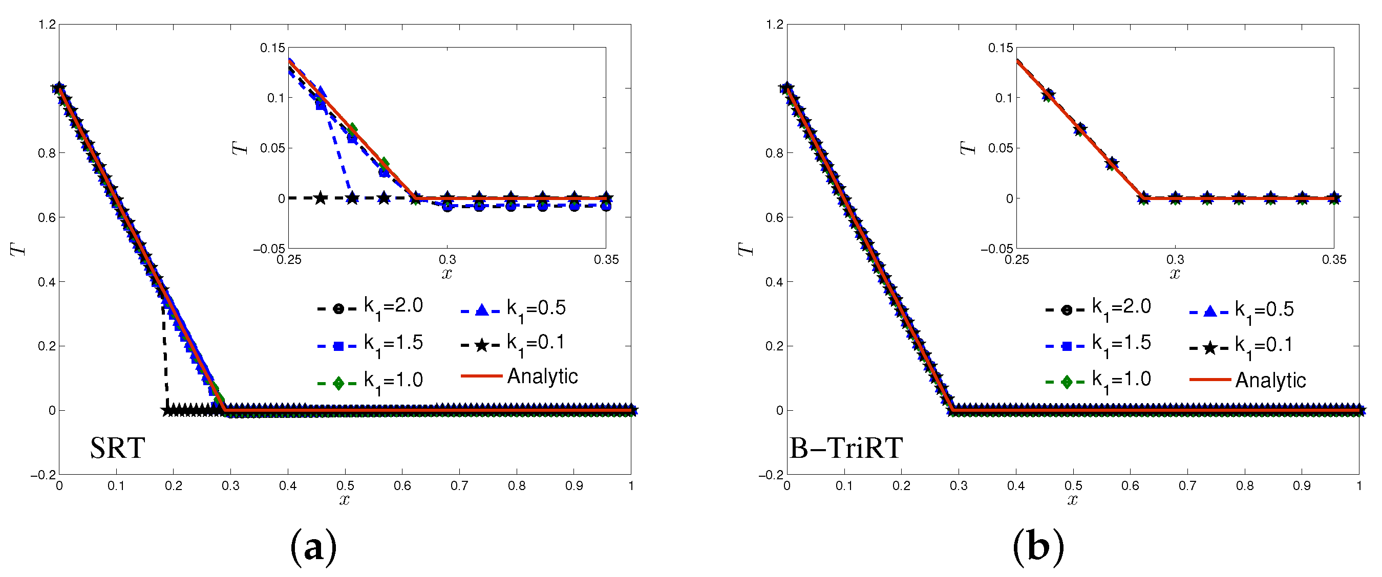
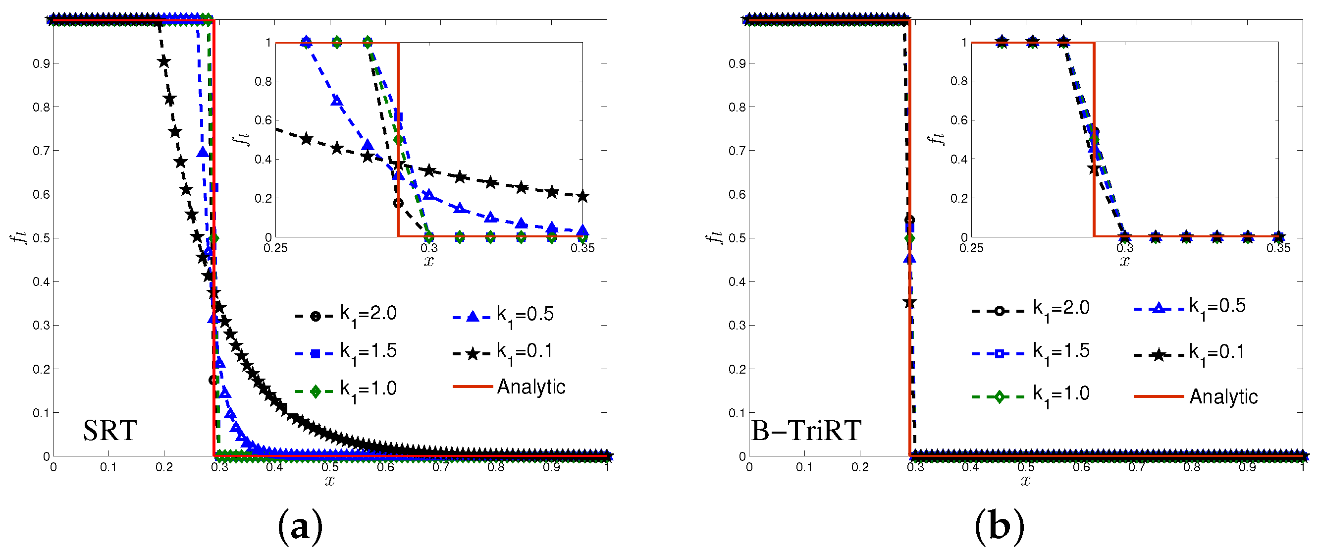
3. Numerical Diffusion Analysis of the B-TriRT LB Model for Solid–Liquid Phase Transition

In this section, we delve into the possible numerical diffusion phenomena at the phase interface in solid–liquid phase transition problems, and we analyze the B-TriRT LB model proposed in this work. Therefore, we will derive a relaxation parameter relationship to eliminate numerical diffusion. Without loss of generality, the one-dimensional isothermal phase transition (melting) problem is considered, where the phase transition temperature is a constant temperature $T_m$ and the solid phase remains at the initial temperature $T_m$. Figure 1 provides a schematic diagram of the macroscopic quantities ($H,f_l,T$) near the solid–liquid interface x point at time t, where the x point is the phase transition interface point, the $x+1$ point is the solid-phase point, and the $x-1$ point is the liquid-phase point.

According to the evolution equation Equation (10), the distribution function of point $x+1$ at time $t+\delta t$ is

$$\begin{array}{cc}\hfill g_i(x+1,t+\Delta t)=& g_i(x,t)-k_0{g}_i^{neq}(x,t)-(k_1-k_0)\frac{{\omega }_i{\mathbf{c}}_i·{\sum }_i{\mathbf{c}}_i(g_i(x,t)-g_i^{eq}(x,t))}{c_s^2}\hfill \\ \hfill & -(k_2-k_0)\frac{{\omega }_i({\mathbf{c}}_i{\mathbf{c}}_i-c_s^2\mathbf{I}):{\sum }_i{\mathbf{c}}_i{\mathbf{c}}_i(g_i(x,t)-g_i^{eq}(x,t))}{2c_s^4},\hfill \end{array}$$

(15)

Then, the evolution equation is divided into the following three categories as

$$\begin{array}{cc}\hfill & g_i(x+{\mathbf{c}}_i{\delta }_t,t+{\delta }_t)=g_i(x,t+{\delta }_t),i=0,2,4;\hfill \\ \hfill & g_i(x+{\mathbf{c}}_i{\delta }_t,t+{\delta }_t)=g_i(x+c{\delta }_t,t+{\delta }_t),i=1,5,8;\hfill \\ \hfill & g_i(x+{\mathbf{c}}_i{\delta }_t,t+{\delta }_t)=g_i(x-c{\delta }_t,t+{\delta }_t),i=3,6,7.\hfill \end{array}$$

(16)

Furthermore, by summing up the distribution functions in the $0,2,4$ directions, $1,5,8$ directions and $3,6,7$ directions, respectively. We can obtain

$$\begin{array}{cc}\hfill & g_0(x,t+{\delta }_t)+g_2(x,t+{\delta }_t)+g_4(x,t+{\delta }_t)\hfill \\ \hfill & =g_0(x,t)+g_2(x,t)+g_4(x,t)-k_0[g_0(x,t)+g_2(x,t)+g_4(x,t)-(g_0^{eq}(x,t)+g_2^{eq}(x,t)\hfill \\ \hfill & +g_4^{eq}(x,t)\left)\right]-(k_0-k_2)[g_1(x,t)+g_5(x,t)+g_8(x,t)-(g_1^{eq}(x,t)+g_5^{eq}(x,t)+g_8^{eq}(x,t))]\hfill \\ \hfill & -(k_0-k_2)[g_3(x,t)+g_6(x,t)+g_7(x,t)-(g_3^{eq}(x,t)+g_6^{eq}(x,t)+g_7^{eq}(x,t))]\hfill \end{array}$$

(17)

$$\begin{array}{cc}\hfill & g_1(x+c{\delta }_t,t+{\delta }_t)+g_5(x+c{\delta }_t,t+{\delta }_t)+g_8(x+c{\delta }_t,t+{\delta }_t)\hfill \\ \hfill & =g_1(x,t)+g_5(x,t)+g_8(x,t)\hfill \\ \hfill & -(\frac{k_1}{2}+\frac{k_2}{2})[g_1(x,t)+g_5(x,t)+g_8(x,t)-(g_1^{eq}(x,t)+g_5^{eq}(x,t)+g_8^{eq}(x,t))]\hfill \\ \hfill & -(\frac{k_2}{2}-\frac{k_1}{2})[g_3(x,t)+g_6(x,t)+g_7(x,t)-(g_3^{eq}(x,t)+g_6^{eq}(x,t)+g_7^{eq}(x,t))]\hfill \end{array}$$

(18)

$$\begin{array}{cc}\hfill & g_3(x-c{\delta }_t,t+{\delta }_t)+g_6(x-c{\delta }_t,t+{\delta }_t)+g_7(x-c{\delta }_t,t+{\delta }_t)\hfill \\ \hfill & =g_3(x,t)+g_6(x,t)+g_7(x,t)\hfill \\ \hfill & -(\frac{k_2}{2}-\frac{k_1}{2})[g_1(x,t)+g_5(x,t)+g_8(x,t)-(g_1^{eq}(x,t)+g_5^{eq}(x,t)+g_8^{eq}(x,t))]\hfill \\ \hfill & -(\frac{k_1}{2}+\frac{k_2}{2})[g_3(x,t)+g_6(x,t)+g_7(x,t)-(g_3^{eq}(x,t)+g_6^{eq}(x,t)+g_7^{eq}(x,t))].\hfill \end{array}$$

(19)

Since $x,t$ are arbitrary values and have generality, we make x in Equation (19) equal to $x+c{\delta }_t$ and t equal to $t-{\delta }_t$. Therefore, Equation (19) can be written as

$$\begin{array}{cc}\hfill & g_3(x,t)+g_6(x,t)+g_7(x,t)\hfill \\ \hfill & =g_3(x+c{\delta }_t,t-{\delta }_t)+g_6(x+c{\delta }_t,t-{\delta }_t)+g_7(x+c{\delta }_t,t-{\delta }_t)\hfill \\ \hfill & -(\frac{k_2}{2}-\frac{k_1}{2})[g_1(x+c{\delta }_t,t-{\delta }_t)+g_5(x+c{\delta }_t,t-{\delta }_t)+g_8(x+c{\delta }_t,t-{\delta }_t)\hfill \\ \hfill & -(g_1^{eq}(x+c{\delta }_t,t-{\delta }_t)+g_5^{eq}(x+c{\delta }_t,t-{\delta }_t)+g_8^{eq}(x+c{\delta }_t,t-{\delta }_t))]\hfill \\ \hfill & -(\frac{k_1}{2}+\frac{k_2}{2})[g_3(x+c{\delta }_t,t-{\delta }_t)+g_6(x+c{\delta }_t,t-{\delta }_t)+g_7(x+c{\delta }_t,t-{\delta }_t)\hfill \\ \hfill & -(g_3^{eq}(x+c{\delta }_t,t-{\delta }_t)+g_6^{eq}(x+c{\delta }_t,t-{\delta }_t)+g_7^{eq}(x+c{\delta }_t,t-{\delta }_t))].\hfill \end{array}$$

(20)

When the point x is the phase transition interface point, $x+1$ is the solid-phase point and $x-1$ is the liquid-phase point; since the temperature at the solid-phase point remains constant, the corresponding distribution function should equal the value of its equilibrium distribution function. Therefore, from Equation (20), it can be obtained that

$$g_3(x,t)+g_6(x,t)+g_7(x,t)=g_3^{eq}(x+c{\delta }_t,t-{\delta }_t)+g_6^{eq}(x+c{\delta }_t,t-{\delta }_t)+g_7^{eq}(x+c{\delta }_t,t-{\delta }_t).$$

(21)

Assuming that at time t a certain point is a solid-phase point, then at time $t-1$, that point must also be a solid-phase point. Meanwhile, due to the constant temperature of the solid-phase point, the equilibrium distribution functions corresponding to the two moments are also identical. Therefore, Equation (21) can be written as

$$g_3(x,t)+g_6(x,t)+g_7(x,t)=g_3^{eq}(x+c{\delta }_t,t)+g_6^{eq}(x+c{\delta }_t,t)+g_7^{eq}(x+c{\delta }_t,t).$$

(22)

Then, substituting Equation (22) into Equation (18) yields

$$\begin{array}{cc}\hfill & g_1(x+c{\delta }_t,t+{\delta }_t)+g_5(x+c{\delta }_t,t+{\delta }_t)+g_8(x+c{\delta }_t,t+{\delta }_t)\hfill \\ \hfill & =g_1^{eq}(x,t)+g_5^{eq}(x,t)+g_8^{eq}(x,t)\hfill \\ \hfill & +(1-\frac{k_1}{2}-\frac{k_2}{2})[g_1(x,t)+g_5(x,t)+g_8(x,t)-(g_1^{eq}(x,t)+g_5^{eq}(x,t)+g_8^{eq}(x,t))]\hfill \\ \hfill & -(\frac{k_2}{2}-\frac{k_1}{2})[g_3^{eq}(x+c{\delta }_t,t)+g_6^{eq}(x+c{\delta }_t,t)+g_7^{eq}(x+c{\delta }_t,t)-(g_3^{eq}(x,t)+g_6^{eq}(x,t)+g_7^{eq}(x,t))].\hfill \end{array}$$

(23)

Since the temperature at the phase transition point remains constant, the corresponding equilibrium distribution function also does not change. Therefore, the above equation can be written as

$$\begin{array}{cc}\hfill & g_1(x+c{\delta }_t,t+{\delta }_t)+g_5(x+c{\delta }_t,t+{\delta }_t)+g_8(x+c{\delta }_t,t+{\delta }_t)\hfill \\ \hfill & =g_1^{eq}(x,t)+g_5^{eq}(x,t)+g_8^{eq}(x,t)\hfill \\ \hfill & +(1-\frac{k_1}{2}-\frac{k_2}{2})[g_1(x,t)+g_5(x,t)+g_8(x,t)-(g_1^{eq}(x,t)+g_5^{eq}(x,t)+g_8^{eq}(x,t))].\hfill \end{array}$$

(24)

In order for the solid-phase point ($x+c{\delta }_t$) to remain inactive, the distribution functions in the directions of $1,5,8$ must satisfy [25]

$$g_1(x+c{\delta }_t,t)+g_5(x+c{\delta }_t,t)+g_8(x+c{\delta }_t,t)=g_1^{eq}(x,t)+g_5^{eq}(x,t)+g_8^{eq}(x,t),$$

(25)

Therefore, the relaxation parameters $k_1$ and $k_2$ should be

$$1-\frac{k_1}{2}-\frac{k_2}{2}=0.$$

(26)

At this point, the numerical diffusion at the interface can be completely eliminated.

4. Numerical Results

4.1. One-Phase Melting by Conduction

We first consider one-phase conduction melting as a benchmark problem to validate the present B-TriRT model’s ability to reduce numerical diffusion across the phase interface. Initially, the phase change material is solid uniformly and the temperature is set to be $T_m$. At time $t>0$, a constant temperature $T_h(T_h>T_m)$ is imposed on the left wall (i.e., $x=0$); then, the phase change material begins to melt. For this problem, the analytical solution of the temperature is given by [25]

$$T(x,t)=\left\{\begin{array}{cc}{T}_h-\frac{(T_h-T_m)erf\left(\frac{x}{2\sqrt{\alpha t}}\right)}{erf\left(\kappa \right)},\hfill & 0<x<X_i\left(t\right),\hfill \\ T_m,\hfill & x>X_i\left(t\right),\hfill \end{array}\right.$$

(27)

where $erf\left(x\right)=\frac{2}{\sqrt{\pi }}{\int }_0^x{e}^{-{\eta }^2}d\eta$ is the error function, and the position of the phase interface can be determined as

$$X_i\left(t\right)=2\kappa \sqrt{\alpha t},\frac{Ste}{exp\left({\kappa }^2\right)erf\left(\kappa \right)}=\kappa \sqrt{\pi }.$$

(28)

In the present simulations, the dimensionless parameters and thermophysical properties are set as $T_h=1,T_m=0,Ste=0.01,\alpha =1/6$, and the computational parameters of present model are given by $\Delta x=1/100,c=1.0$. In addition, the time step $\Delta t$ is calculated by the relationship $\Delta t=\alpha /\left[c_s^2(1/k_1-0.5)\right]$, with $k_1$ being set as $0.1,0.5,1.0,1.5$ and $2.0$, respectively. The temperature distributions at $t=25$ of the SRT model and the present B-TriRT model for different $k_1$ values are illustrated in Figure 2. It can be seen from Figure 2a that for the SRT model, the temperature distributions deviate from the analytical solutions when $k_1\ne 1$. The results show that the solid phase has been activated before it starts melting, which can be explained by the numerical diffusion [25]. However, for the present B-TriRT model, the temperature distributions agree well with the analytical solutions, and the temperatures of the solid phase stay at $T_m$. The results indicate that the numerical diffusion across the phase interface can be dramatically reduced when employing the present B-TriRT model. On the other hand, as discussed in ref. [25], the numerical diffusion will cause the phase interface width to exceed one lattice spacing. To verify this point clearly, the liquid fraction distributions at $t=25$ are captured by the SRT model and the present B-TriRT model with different $k_1$ values, and the results are shown in Figure 3. The results indicate that the phase interface width obtained from the SRT model is always larger than one lattice spacing. However, the phase interface width obtained by the present B-TriRT model is exactly one lattice spacing. From the above results and discussions, it can be concluded that the present B-TriRT model can be exploited to reduce the numerical diffusion across the phase interface in the solid–liquid phase change problem.

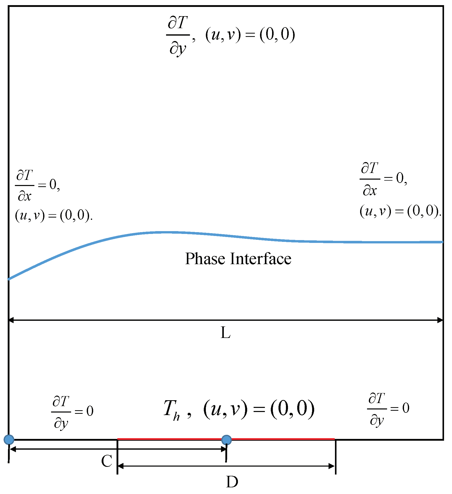
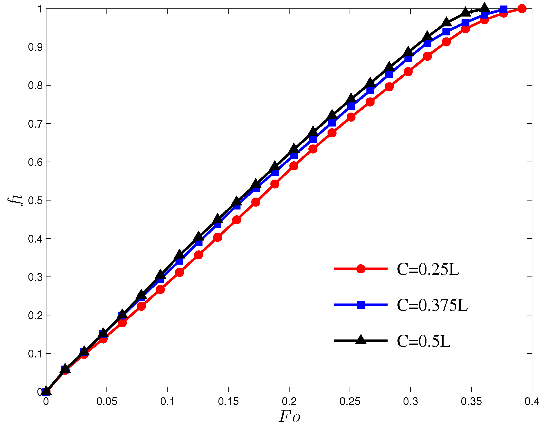
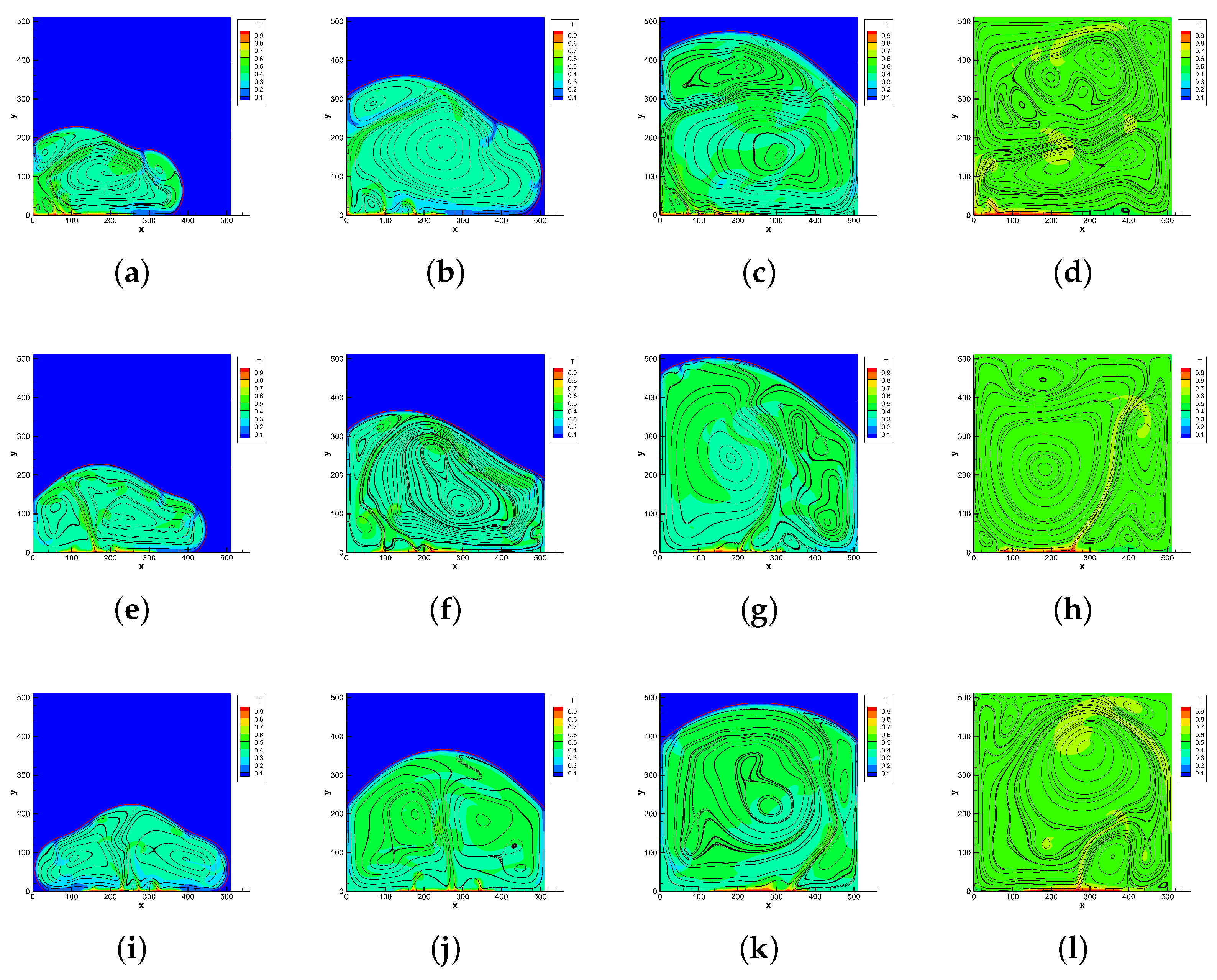
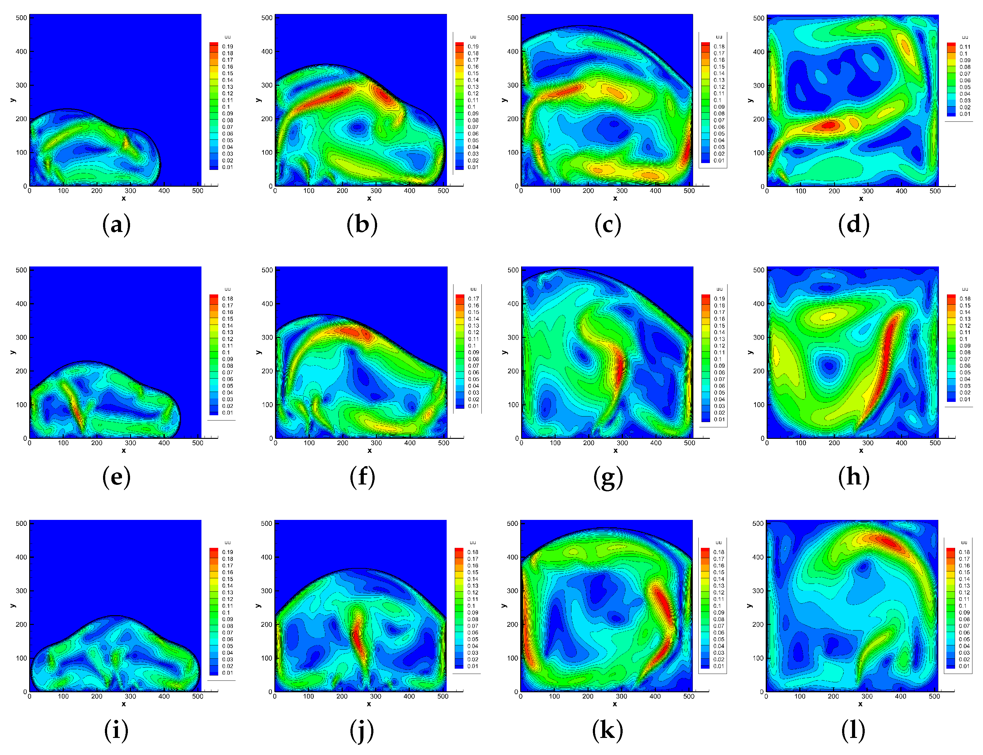
4.2. Melting in a Cavity Heated Locally from Below

In this section, melting in a cavity heated locally from below is investigated. As shown in Figure 4, the problem consists of a cubical cavity with length $L=1.0$ that is filled with PCM at the initial temperature $T_m$, and the cavity is heated locally with temperature $T_h$ from below. The width of the heated region is set to $D=0.5L$, and the distance from the left wall to the center of heated region (C) is varied in the range of $0.25⩽C⩽0.5$. For the walls of the cavity, non-slip adiabatic boundary conditions (i.e., $\partial T/\partial \mathbf{n}=0,(u,v)=(0,0)$, where $\mathbf{n}$ is the normal vector of walls) are applied.

In the present investigation, we consider the influence of C on the melting process, and we plot the liquid fraction variation for different cases in Figure 5, where $T_h=1$, $T_m=0,Ra={10}^8,Pr=6.2,Ste=0.125,c=1.0,\Delta x=1/512$. As shown in Figure 5, when the distance C is changed from 0.25L to 0.5L, the full melting time is decreased. The results indicate that the melting rate can be increased through changing the heated region from the sides to the middle region. The reason can be interpreted by a symmetry argument. The average distance between the PCM and the heated region is minimized when the heated region is centered, which allows faster melting. Furthermore, the instantaneous flow and temperature structures and the contours of the flow field are presented in Figure 6 and Figure 7. From these figures, it can be observed that the flow in the melt region is nearly chaotic, with a thin thermal boundary layer. In addition, the interface area in the case of C = 0.5L is larger than the interface area in the cases of $C=0.25L$ and $C=0.375L$, which leads to a larger melting rate at $C=0.5L$.

5. Conclusions

In this study, a B-TriRT model was developed to address the solid–liquid phase change problem. Through considering a one-dimensional isothermal phase transition problem, a relaxation parameter relationship was derived that can mitigate numerical diffusion across the phase interface significantly. The numerical experiment of one-phase melting by conduction confirmed that the numerical diffusion across the phase interface can be dramatically reduced by the present B-TriRT model. Furthermore, we examined the effects of the heated region’s location on the melting process at high Rayleigh numbers. The results indicate that positioning the heated region at the center of the bottom wall facilitates earlier complete melting.

References

1. Zhang, N.; Yuan, Y.; Cao, X.; Du, Y.; Zhang, Z.; Gui, Y. Latent heat thermal energy storage systems with solid–liquid phase change materials: A review. Adv. Eng. Mater. 2018, 20, 1700753. [Google Scholar] [CrossRef]
2. Tomita, S.; Celik, H.; Mobedi, M. Thermal analysis of solid/liquid phase change in a cavity with one wall at periodic temperature. Energies 2021, 14, 5957. [Google Scholar] [CrossRef]
3. Malik, M.; Dincer, I.; Rosen, M. Review on use of phase change materials in battery thermal management for electric and hybrid electric vehicles. Int. J. Energy Res. 2016, 40, 1011–1031. [Google Scholar] [CrossRef]
4. Konuklu, Y.; Ostry, M.; Paksoy, H.; Charvat, P. Review on using microencapsulated phase change materials (PCM) in building applications. Energy Build. 2015, 106, 134–155. [Google Scholar] [CrossRef]
5. Shirbani, M.; Siavashi, M.; Bidabadi, M. Phase Change Materials Energy Storage Enhancement Schemes and Implementing the Lattice Boltzmann Method for Simulations: A Review. Energies 2023, 16, 1059. [Google Scholar] [CrossRef]
6. Chen, D.; Riaz, A.; Aute, V.; Radermacher, R. A solid-liquid model based on lattice Boltzmann method for phase change material melting with porous media in cylindrical heat exchangers. Appl. Therm. Eng. 2022, 207, 118080. [Google Scholar] [CrossRef]
7. Chiappini, D. A coupled lattice Boltzmann-finite volume method for phase change material analysis. Int. J. Therm. Sci. 2021, 164, 106893. [Google Scholar] [CrossRef]
8. Rui, Z.; Li, J.; Ma, J.; Cai, H.; Nie, B.; Peng, H. Comparative study on natural convection melting in square cavity using lattice Boltzmann method. Results Phys. 2020, 18, 103274. [Google Scholar] [CrossRef]
9. Chen, Z.; Shu, C.; Yang, L.; Zhao, X.; Liu, N. Phase-field-simplified lattice Boltzmann method for modeling solid-liquid phase change. Phys. Rev. E 2021, 103, 023308. [Google Scholar] [CrossRef]
10. Han, Q.; Wang, H.; Yu, C.; Zhang, C. Lattice Boltzmann simulation of melting heat transfer in a composite phase change material. Appl. Therm. Eng. 2020, 176, 115423. [Google Scholar] [CrossRef]
11. Feng, Y.; Li, H.; Li, L.; Bu, L.; Wang, T. Numerical investigation on the melting of nanoparticle-enhanced phase change materials (NEPCM) in a bottom-heated rectangular cavity using lattice Boltzmann method. Int. J. Heat Mass Transf. 2015, 81, 415–425. [Google Scholar] [CrossRef]
12. Chen, S.; Doolen, G. Lattice Boltzmann method for fluid flows. Annu. Rev. Fluid Mech. 1998, 30, 329–364. [Google Scholar] [CrossRef]
13. Qian, Y.; Succi, S.; Orszag, S. Recent advances in lattice Boltzmann computing. Annu. Rev. Comput. Phys. 1995, 3, 195–242. [Google Scholar]
14. d’Humières, D. Generalized lattice-Boltzmann equations, in: Rarefied gas dynamics: Theory and simulations. Progress Astronaut. Aeronaut. 1992, 159, 450–458. [Google Scholar]
15. Lallemand, P.; Luo, L. Theory of the lattice Boltzmann method: Dispersion, dissipation, isotropy, Galilean invariance, and stability. Phys. Rev. E 2000, 61, 6546. [Google Scholar] [CrossRef]
16. Guo, Z.; Shu, C. Lattice Boltzmann Method and Its Applicatons in Engineering; World Scientific Publishing: Singapore, 2013. [Google Scholar]
17. Isfahani, A.H.; Tasdighi, I.; Karimipour, A.; Shirani, E.; Afrand, M. A joint lattice Boltzmann and molecular dynamics investigation for thermohydraulical simulation of nano flows through porous media. Eur. J. Mech. B-Fluids 2016, 55, 15–23. [Google Scholar] [CrossRef]
18. Chai, Z.; He, N.; Guo, Z.; Shi, B. Lattice Boltzmann model for high-order nonlinear partial differential equations. Phys. Rev. E 2018, 97, 013304. [Google Scholar] [CrossRef]
19. Chai, Z.; Shi, B. Multiple-relaxation-time lattice Boltzmann method for the Navier-Stokes and nonlinear convection-diffusion equations: Modeling, analysis, and elements. Phys. Rev. E 2020, 102, 023306. [Google Scholar] [CrossRef]
20. Shi, B.; Guo, Z. Lattice Boltzmann model for nonlinear convection-diffusion equations. Phys. Rev. E 2009, 79, 016701. [Google Scholar] [CrossRef] [PubMed]
21. Qiao, Z.; Yang, X.; Zhang, Y. Mass conservative lattice Boltzmann scheme for a three-dimensional diffuse interface model with Peng-Robinson equation of state. Phys. Rev. E 2018, 98, 023306. [Google Scholar] [CrossRef] [PubMed]
22. Yang, X.; Shi, B.; Chai, Z.; Guo, Z. A Coupled Lattice Boltzmann Method to Solve Nernst-Planck Model for Simulating Electro-osmotic Flows. J. Sci. Comput. 2014, 61, 222–238. [Google Scholar] [CrossRef]
23. Wang, L.; He, K.; Wang, H. Phase-field-based lattice Boltzmann model for simulating thermocapillary flows. Phys. Rev. E 2023, 108, 055306. [Google Scholar] [CrossRef] [PubMed]
24. Zhao, Y.; Pereira, G.; Kuang, S.; Chai, Z.; Shi, B. A generalized lattice Boltzmann model for solid-liquid phase change with variable density and thermophysical properties. Appl. Math. Lett. 2020, 104, 106250. [Google Scholar] [CrossRef]
25. Huang, R.; Wu, H. Phase interface effects in the total enthalpy-based lattice Boltzmann model for solid-liquid phase change. J. Comput. Phys. 2015, 294, 346–362. [Google Scholar] [CrossRef]
26. Liu, Q.; Wang, X.; Feng, X.; Liu, F. An enthalpy-based cascaded lattice Boltzmann method for solid-liquid phase-change heat transfer. Appl. Therm. Eng. 2022, 209, 118283. [Google Scholar] [CrossRef]
27. Liu, X.; Tong, Z.; He, Y. Enthalpy-based immersed boundary-lattice Boltzmann model for solid-liquid phase change in porous media under local thermal non-equilibrium condition. Int. J. Therm. Sci. 2022, 182, 107786. [Google Scholar] [CrossRef]
28. Xu, X.; He, Y.; Han, J.; Zhu, J. Multiple-relaxation-time lattice Boltzmann model for anisotropic liquid-solid phase change. Appl. Math. Lett. 2022, 134, 108358. [Google Scholar] [CrossRef]
29. Zhao, Y.; Wu, Y.; Chai, Z.; Shi, B. A block triple-relaxation-time lattice Boltzmann model for nonlinear anisotropic convection-diffusion equations. Comput. Math. Appl. 2020, 79, 2550–2573. [Google Scholar] [CrossRef]
30. Zhao, Y.; Wu, Y.; Chai, Z.; Shi, B. Lattice Boltzmann simulations of melting in a rectangular cavity heated locally from below at high Rayleigh number. arXiv 2019, arXiv:1909.13086. [Google Scholar]
Figure 1. Schematic diagram of macroscopic quantities ( H , f l , T ) near point x at the solid–liquid interface at time t.
Mathematics 12 01815 g001
Figure 2. Comparisons of temperature distributions between SRT model (a) and B-TriRT model (b) for different k 1 values.
Mathematics 12 01815 g002
Figure 3. Comparisons of liquid fraction distributions between SRT model (a) and B-TriRT model (b) for different k 1 values.
Mathematics 12 01815 g003
Figure 4. Schematic illustration of the physical domain.
Mathematics 12 01815 g004
Figure 5. The variation of fractions for different cases at different F o values.
Mathematics 12 01815 g005
Figure 6. The streamlines and contours of the temperatures for the different cases at different F o values. ((ad): C = 0.25 L , (eh): C = 0.375 L and (il): C = 0.5 L ; (a,e,i): F o = 0.1 , (b,f,j): F o = 0.2 , (c,g,k): F o = 0.3 and (d,h,l): F o = 0.4 ). The phase interface is marked by the red line.
Mathematics 12 01815 g006
Figure 7. The contours of the velocities at different F o values. ((ad): C = 0.25 L , (eh): C = 0.375 L and (il): C = 0.5 L ; (a,e,i): F o = 0.1 , (b,f,j): F o = 0.2 , (c,g,k): F o = 0.3 and (d,h,l): F o = 0.4 ).
Mathematics 12 01815 g007
Disclaimer/Publisher’s Note: The statements, opinions and data contained in all publications are solely those of the individual author(s) and contributor(s) and not of MDPI and/or the editor(s). MDPI and/or the editor(s) disclaim responsibility for any injury to people or property resulting from any ideas, methods, instructions or products referred to in the content.