Predicting Stroke Risk Based on ICD Codes Using Graph-Based Convolutional Neural Networks

Abstract

In recent years, convolutional neural networks (CNNs) have emerged as highly efficient architectures for image and audio classification tasks, gaining widespread adoption in state-of-the-art methodologies. While CNNs excel in machine learning scenarios where the data representation exhibits a grid structure, they face challenges in generalizing to other data types. For instance, they struggle with data structured on 3D meshes (e.g., measurements from a network of meteorological stations) or data represented by graph structures (e.g., molecular graphs). To address such challenges, the scientific literature proposes novel graph-based convolutional network architectures, extending the classical convolution concept to data structures defined by graphs. In this paper, we use such a deep learning architecture to examine graphs defined using the ICD-10 codes appearing in the medical data of patients who suffered hemorrhagic stroke in Hungary in the period 2006–2012. The purpose of the analysis is to predict the risk of stroke by examining a patient’s ICD graph. Finally, we also compare the effectiveness of this method with classical machine learning classification methods. The results demonstrate that the graph-based method can predict the risk of stroke with an accuracy of over 73%, which is more than 10% higher than the classical methods.

1. Introduction

Nowadays, with the rapid emergence of deep learning solutions, significant advances are being made in data analyses and related predictive analytics. Every day, we see artificial intelligence making inroads into more and more areas of life and being integrated into institutions such as medical research institutes, businesses and police stations, significantly improving people’s quality of life.

The importance of neural networks in machine learning is unquestionable, as their application makes it easy to identify correlations in data. Convolutional neural networks (CNNs), based on convolutional operations, have become increasingly popular in image analysis and audio recognition, as they can be used to easily extract hidden information from data [1,2,3]. However, while CNNs excel on gridded data such as images, it remains challenging to generalize them to other data types, such as 3D meshes or graphs. This problem arises from the fact that graphs cannot be used directly as input to neural networks due to their non-Euclidean nature but must first be embedded in an n-dimensional vector space [4].

Significant advances have also been made in the analysis of health data using deep learning. Graph-based convolutional neural networks (GCNNs) have shown promise for the analysis of health data, particularly for disease prediction. In addition, these models have applications in many other areas, such as the analysis of chemical structures, the modeling of social networks and the study of biological networks. CNNs have led to significant improvements in the analysis of graph-structured datasets, allowing the exploration and exploitation of complex relationships in such data [5].

Today, hemorrhagic stroke is one of the most common and severe types of cerebrovascular accidents and one of the most common causes of death worldwide, with a significant proportion of survivors suffering severe disability, often manifested as impaired mobility and speech. The most common type of hemorrhagic stroke occurs when a blood vessel inside the brain bursts and blood leaks into the surrounding brain tissue (intracerebral hemorrhage). The bleeding causes the death of brain cells, and the affected part of the brain does not function properly. It is, therefore, crucial to predict the risk of hemorrhagic stroke, as it requires immediate medical intervention and, if not treated, can cause long-term neurological damage and, in many cases, death [6,7].

In this study, we investigate how a patient’s medical history can be used to predict the occurrence of a hemorrhagic stroke within a given time frame, thus supporting its prevention. To this end, we investigate the effectiveness of GCNNs in predicting stroke risk based on ICD-10 codes and perform a comparative analysis comparing the performance of GCNNs with classical machine learning classification methods.

2. Related Work

The development of artificial intelligence is a major step forward for medicine. Research and scientific work are emerging every day in this field, providing solutions for preventing, diagnosing or predicting diseases. In this section, we present recent machine learning-based work that has been used to predict stroke risk.

Various data modalities have been used to predict stroke using machine learning tools, such as retinal images [8] or numerical cardiovascular data analysis [9]. In [9], on cardiovascular data, classical machine learning methods were used to predict stroke. For example, using an SVM classifier, it achieved an AUC of 0.751. In [8], convolutional neural networks were used based on the retinal vasculature and achieved an AUC of 0.699 for the database under study.

In [10], machine learning algorithms were successfully used to accurately identify the type of stroke that has already occurred or may occur. The study employed four different algorithms: Naive Bayes, J48, K-Nearest Neighbor (KNN) and Random Forest. The researchers used data collected from hospitals, which included a range of features, such as patient age, gender, vision loss, dizziness, headache, weakness, nausea, vomiting, loss of balance, irregular heartbeat, chest pain and fatigue. The classification results were satisfactory, allowing for their use in real-time medical reports. The Naive Bayes classifier accuracy was found to be 85.6%.

Research on stroke classification has also used approaches combining different text mining tools and machine learning algorithms. In one study [11], case records of 507 patients from Sugam Multispecialty Hospital, Kumbakonam, Tamil Nadu, India, were collected and analyzed using these methods. Labeling and maximum entropy methods were used to extract the symptoms from the case sheets, and then a derivation algorithm was used to extract common and unique attributes for stroke classification. The processed data were tested using various machine learning algorithms, such as artificial neural networks, SVM, boosting and bagging methods and random forests.

Another study [12] used electronic health records (EHRs) to attempt to predict stroke risk. They used data from 29,072 patients published by McKinsey & Company and available on Kaggle to investigate the impact of risk factors on stroke prediction. The data included patient gender, age, hypertension, heart disease, blood glucose and smoking status. Of the algorithms, the feed-forward multi-layer perceptron achieved the best accuracy of 75.02%, while the decision tree and Random Forest had similar performance. The authors concluded that neural networks can efficiently handle multivariate and noisy data.

Using the Cardiovascular Health Study (CHS) dataset, another study [13] applied a decision tree algorithm for feature selection, principal component analysis for dimension reduction, and a back-propagation neural network for classification. The dataset includes data from 5457 men and women who were examined annually between 1989 and 1999 using various medical tests, such as MRI, ambulatory electrocardiograms and questionnaires. Their model was found to be highly effective in predicting stroke.

The authors of [14] investigated various physiological parameters used as risk factors for predicting stroke. Data were collected from the International Stroke Trial database and successfully trained and tested using SVM. In their research, the authors implemented SVM using different kernel functions and found that the linear kernel provided 90% accuracy.

In [15], a graph convolutional neural network was used to predict autism spectrum disorder and Alzheimer’s disease. The study represented the populations as a sparse graph, where nodes are associated with imaging feature vectors, while phenotypic information is integrated as the edge of the graph. This framework significantly outperformed other methods on both the ABIDE and ADNI datasets, with classification accuracies of 70.4% and 80.0%, respectively.

As we will see, we use the graph generated from the patient’s visit to the doctor for prediction. This has the advantage that, after each visit, this graph expands, and with this graph, the doctor can use our framework in real time to check for suspected hemorrhagic stroke.

3. Methodology

3.1. Neural Networks

Artificial neural networks (ANNs) are biologically inspired systems that can be defined as adaptive tools for parallel processing to solve computational problems. These models consist of artificial neurons that communicate with each other in layers through nonlinear activation functions.

However, when the data have a graph structure, such as molecular graphs or social networks, traditional neural networks cannot handle the data efficiently, and the prediction accuracy is significantly reduced. To address this problem, graph-based convolutional neural networks have emerged.

3.2. Graph Convolutional Neural Networks

3.2.1. Graphs

In real life, many situations can be well modeled using diagrams that consist of a set of points, and these points are connected by one or more lines. For example, human relationships (and social network models) can be described using such models, where the points represent people, and the lines represent the relationship between them. The strength of the connection can be characterized by assigning an appropriate weight to each line. In the social network model, people are represented as points (or nodes), and the more important a person is, the more weight we can attach to the node that represents him/her. In a social network, people’s influence on one another can be linked by weighted lines. In addition to the strength of the relationship, the direction of the relationship (directional lines) also emerges as an important factor. A mathematical abstraction tool for modeling such real situations is the graph.

A graph G is a tuple $(V,E,\phi )$, where $V=\{v_1,\dots ,v_p\}$ is a finite set whose elements are called nodes (or vertices), the finite set E is the set of edges, and $\phi$ is a mapping from E to the set of ordered (in the case of a directed graph) or unordered pairs (in the case of undirected graphs). In the rest of the paper, we restrict ourselves to the use of simple undirected graphs (i.e., we do not allow multiple edges and loop edges). If $\phi :e\mapsto \{u,v\}$, we say that the edge e connects the vertices u and v. In the case of simple undirected graphs, we can just write $e=\{u,v\}$ for the edge connecting u and v.

One of the most common ways to represent graphs on computers is the use of the adjacency matrix, which is a $p\times p$ matrix A defined by $A=\left(a_{ij}\right)$, where $a_{ij}:=1$ if $u_i$ and $u_j$ are connected by an edge, and $a_{ij}=0$ otherwise.

A graph is called an edge-weighted graph if a weight (a number) is associated with each of its edges. This weight can represent cost, length, frequency, etc., depending on the particular problem. Let us use $w_{ij}$ to denote the weight of the edge $\{u_i,u_j\}$, and we put $w_{ij}=0$ if $u_i$ and $u_j$ are not connected by an edge. (Note that since we assume the graph to be undirected, we have $w_{ij}=w_{ji}$ for all possible pairs of indices $i,j$.) If we consider an edge-weighted graph, we can represent it by its weighted adjacency matrix $W={\left(w_{ij}\right)}_{1\le i,j\le p}$ (see Figure 1).

3.2.2. Graph Convolutional Neural Networks and Graph Embedding

Graph convolutional neural networks (GCNNs) are deep learning models designed to analyze datasets containing graph structures. These models employ a novel approach compared to traditional convolutional neural networks, as they can directly process and analyze graph-structured data, such as social networks, molecular structures or geographic data. The innovation of GCNNs lies in their ability to extract the structural and topological features of graphs by applying convolution operations to adjacent nodes and edges. This allows complex relationships and patterns within graphs to be learned and used for various tasks, such as node or edge classification, prediction and representation [16].

An important aspect of applying GCNNs is graph embedding. Graph embedding aims to transform graphs into spatial representations that machine learning algorithms can efficiently handle. The point of using such graph embedding techniques is, therefore, to assign low-dimensional Euclidean vectors to graphs such that the representations of structurally similar graphs are close to each other in the embedded space. This results in more efficient and scalable machine learning solutions on graph-structured data [16,17].

Commonly used graph embedding methods include Word2Vec, DeepWalk, node2vec and GraphSAGE. These methods employ various algorithms to embed the nodes and edges of graphs, allowing for the learning and representation of relationships and patterns within the graphs [17].

3.2.3. GCNN and PATCHY-SAN

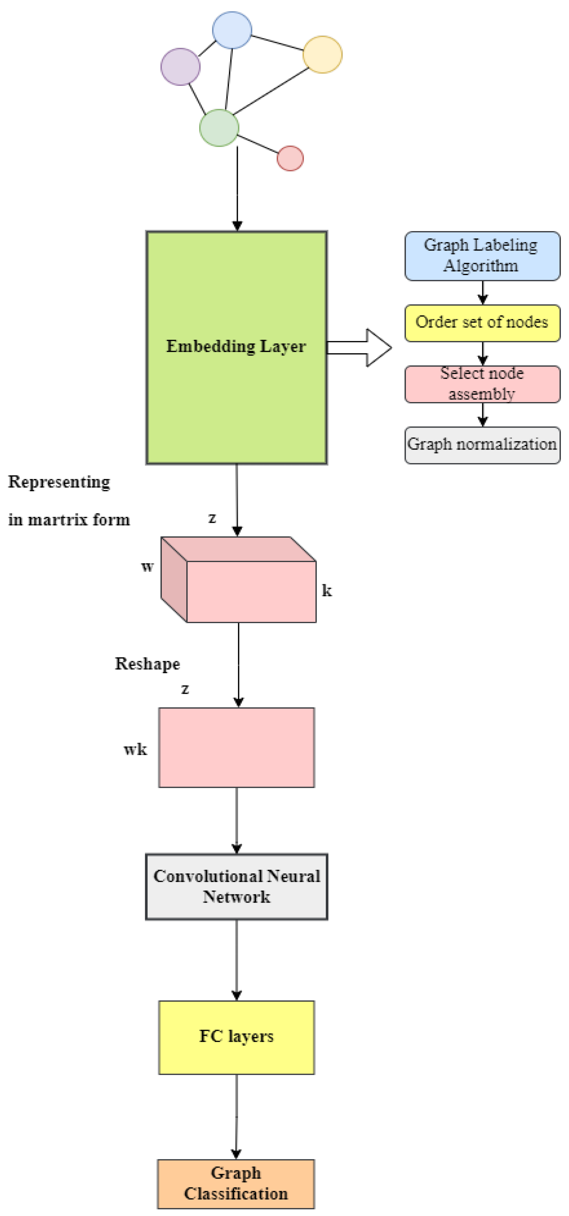
One innovative approach to graph convolutional neural networks was investigated by Niepert et al. [18]. Their methodology, known as PATCHY-SAN, addresses the problems encountered with the graphs mentioned earlier. They presented a framework for training convolutional neural networks on different graph structures, including undirected and directed graphs. Furthermore, they outlined a universal method for extracting spatially connected regions from graphs, similar to image-based convolutional networks that analyze spatially connected regions in images. For each graph, this method involves three main steps: selecting the order of nodes, compiling neighborhoods and normalizing the graph.

The first step is to label the vertices and then sort the nodes based on the resulting values. After selecting the appropriate convolutional vertices, an object called a neighborhood graph is created for that vertex to implement the graph embedding. The next step is to normalize the graph, which imposes an order on the nodes of the neighborhood graph to map from the unordered graph space to a vector space with a linear order. After running the algorithm, the result is a vector-embedded vertex.

4. Dataset Description

In Hungary, the healthcare system is based on a single state-owned insurance organization, the National Health Insurance Fund. Each Hungarian citizen at the time of birth is allocated a unique social security number, and all medical data concerning this person are registered in a database and connected to his or her social security number. The healthcare providers (hospitals, clinics, family doctors, etc.) are reimbursed by the National Health Insurance Fund for their services. To register the provided services in the central database, the 10th International Classification of Diseases (ICD-10) is used, where each disease has a specific code. At each visit, the doctor registers the corresponding code of each diagnosed and/or treated disease of the patient under the social security number of the patient. Thus, in Hungary, there exists an extensive database of medical data of the population. For our investigations, we used data obtained from the NEUROHUN database, which was created in the frame of the Hungarian Brain Research Program. The current investigation included the records of all patients whose primary diagnosis was hemorrhagic stroke (ICD codes I60, I61, I62) in one of their inpatient or outpatient care medical reports in the period 2006–2012. The medical data from three years before and after the hemorrhagic stroke were available for the patients included in the dataset. Our database contained the data of 57,052 patients.

4.1. Data Cleaning and Preprocessing

For the purpose of our analysis, we used only the first three digits of the ICD-10 codes recorded for a patient visit. These three digits reflect the main disease categories, so this modification led to a more concise set of data. All outpatient visits with their respective ICD-10 codes were considered separate visits, while every inpatient case was regarded as a single visit, with the first day of the inpatient stay considered the date of that given visit. Whenever outpatient visits occurred during the inpatient care of a given patient, the ICD-10 codes recorded for these outpatient visits were considered to belong to the inpatient case. Altogether, the data of a given patient contained the dates of visits, the relative times of visits (e.g., the time in reference to the index hemorrhagic stroke) and all ICD-10 diagnosis codes reported by the doctor with respect to the visit for the purpose of reimbursement.

In 1989, different five-digit ICD-10 codes were registered during the period of observation. From these, we omitted ICD-10 codes that belong to the following categories:

• R00–R99: Symptoms, signs and abnormal clinical and laboratory findings.
• S00–T98: Injury, poisoning and certain other consequences of external causes.
• V01–Y98: External causes of morbidity and mortality.
• Z00–Z99: Factors influencing health status and contact with health services
• U00–U85: Codes for special purposes, since they do not code specific diseases.

Due to their low prevalence, codes belonging to the following categories were also excluded:

• P00–P96: Certain conditions originating in the perinatal period.
• Q00–Q99: Congenital malformations, deformations and chromosomal abnormalities.

The remaining 1088 disease codes in “A-O” ICD-10 code categories were included in the investigation.

4.2. Data Construction

Based on our database, we defined two graphs corresponding to each patient. The first graph (let us denote it by H) was created with respect to the period starting 1460 days before the stroke and ending 730 days before the stroke, while the second graph (denoted by G) was created with respect to the period of 365 days preceding the day of the stroke. The vertices of each graph are the ICD codes of every disease diagnosed during all inpatient and outpatient visits of the corresponding patient during the given period. An edge connects two such vertices if the respective codes have been included in a report of the same visit. The weight of an edge is the number of visits in which the codes corresponding to the two connected vertices appeared together in the reports. We note that, in many cases, the disease graph for a particular patient may depend on the way the patient’s doctor works. Some doctors will perform more tests, while others will perform fewer in a given situation. Thus, a patient will have more or fewer ICD-10 codes, depending on the doctor.

Figure 2 shows some steps of creating the graph G for a given patient who had an increasing number of medical checkups (visits) before they suffered a hemorrhagic stroke. Clearly, with each of these checkups, the patient graph increases. The first image shows the graph after including the data from the first visit during the last year before the stroke; the second picture shows the graph after including the data from the first four visits, etc. Finally, the last graph in Figure 2 shows the final form of the graph G, i.e., the graph after the last visit before the stroke. The graph G corresponds to the patient we used in our investigations. In Figure 2, one can see that, at the beginning, only codes between F01 and F99 (Mental, Behavioral and Neurodevelopmental disorders) appeared in the graph. Later, these were extended by codes between I00 and I99 (Diseases of the circulatory system).

Based on the above, training and test datasets for a graph-based neural network were created using data from 57,052 patients to predict the risk of hemorrhagic stroke. The division was based on the assumption, consistent with medical advice, that most signs of strokes occur or are amplified within a year before the incident. Accordingly, the graphs marked H above were considered to belong to healthy patients for whom the onset of a stroke is not yet predictable. However, in the year preceding a stroke, there are already signs that may indicate the onset of the disease, and therefore, graphs from this period, marked G above, are labeled as having a risk of stroke.

In addition to predicting the risk of hemorrhagic stroke, we also address another problem, which focuses on the investigation of fatal/non-fatal cases. For this, we have less data available, with a total of 34,210 patients for whom the outcome of stroke is available, so we will discuss this as a separate case and investigate it with a model architecture that fits the dataset.

We used 70% of the dataset for training, 20% for testing and 10% for validation.

5. Our Method

5.1. Graph-Based Convolutional Neural Network Approach

As a proprietary approach, we developed a graph convolution architecture to maximize prediction accuracy. The first step was to choose the type and number of layers in the model. To this end, we started testing with a simple and shallow architecture and gradually increased the complexity and depth of the architecture until satisfactory performance was achieved. An important task was to find the optimal parameters of the model to design the right architecture, such as the learning rate, number of epochs, number of units, kernel size, dropout rate, regularization coefficient and tuning of the activation function. For hyperparameter optimization, we used the Hyperopt Python library to determine the optimal values of these parameters to maximize model performance and minimize model overfitting.

To embed the graphs of the ICD codes, we used the PATCHY-SAN method described in [18] and integrated it into our GCNN architecture. The adjacency matrix is used to represent the graphs and is passed to the embedding algorithm, which can perform a kind of dimensionality reduction by mapping the relationships in the graph but not in the usual graph embedding terminology. The PATCHY-SAN method has several advantages over other approaches. On the one hand, it is highly efficient and naively parallelizable. On the other hand, PATCHY-SAN is applicable to large graphs, and it learns application-dependent features without the need for feature engineering.

The algorithm executes the subsequent steps for every input graph. The first step is to perform the graph embedding process, where the graph embedding algorithm identifies several nodes and determines their order. Subsequently, a neighborhood graph comprising precisely k nodes is extracted for each of these designated nodes. Next, the neighborhood graphs undergo normalization, meaning that each graph is distinctly mapped to a space possessing a predetermined linear order. This process is indispensable, as the normalized neighborhood graphs will function as the receptive fields for the corresponding node. Ultimately, these normalized neighborhood graphs serve as the receptive fields for the CNN, whereby they are integrated with appropriate feature learning components, specifically convolutional layers and dense layers. After the graph embedding, our convolutional architecture extracts the hidden information from the graph, and then the fully connected layer is used to form the corresponding outputs for classification (see Figure 3).

5.2. Model Design and Parameter Settings

To describe network architectures, we use the following notation: a fully connected layer with k hidden units is denoted by FCk, while a pooling layer of size and stride k is represented by Pk. Additionally, GCk signifies a graph convolutional layer with k feature maps. In our architecture, all GCk and FCk layers are followed by a ReLU activation function. The final layer always consists of softmax regression (see

Table 1. Proposed graph convolution architecture.

Dataset	Architecture
Stroke risk	GC64-GC128-P2-GC256-P2-GC128-P2-GC64-FC128-FC64-SoftMax
Fatal and non-Fatal	GC64-GC64-P3-GC256-P2-GC512-FC32-SoftMax

). The loss energy in the softmax layer is defined in terms of the cross-entropy, and the size of the minibatches we use is 32. We extract neighborhood graphs for 15 selected nodes, with a neighborhood size of 5.

During training, we utilized 10-fold cross-validation with the training set for model validation by randomly splitting the dataset. We employed a batch size of 64 to facilitate the learning process and optimize training time. Another important element is the use of dropout between layers with a ratio of 0.3 to avoid overfitting. The training duration spanned 82 epochs for stroke prediction and 27 epochs for fatal/non-fatal prediction, with the aim of mitigating overfitting. We adopted binary cross-entropy as the loss function of our model with a learning rate of ${10}^{-4}$ to minimize model loss. The combination of our binary cross-entropy loss function and Adam optimizer allowed us to efficiently and quickly train our graph-based convolutional neural network for binary classification tasks. These choices were well suited to our specific problem.

5.3. Evaluation of the Model

To evaluate the model, we calculated the frequently used performance measures: sensitivity, specificity, precision and accuracy. Accuracy can be obtained as follows: Let T be the set of test cases and the size of the set be S. Furthermore, let $G_i$ be an element of the set T with class label $y_i$ and let the class predicted by the GCNN be $\widehat{y_i}$. The accuracy can then be calculated as follows:

$$Accuracy=\frac{{\sum }_{i=1}^S\delta (y_i=\widehat{y_i})}{S}$$

(1)

where $\delta (·)=1$ if the condition is true and 0 otherwise.

Precision is calculated using the following formula:

$$Precision=\frac{TP}{TP+FP}$$

(2)

where TP (true positive) corresponds to the number of positive cases correctly predicted by the classification model, and FP (false positive) corresponds to the number of negative cases incorrectly predicted as positive by the classification model.

Sensitivity, also known as recall, measures the proportion of correctly predicted positive cases by the model. It is calculated using the following formula:

$$Sensitivity=\frac{TP}{TP+FN}$$

(3)

where FN (false negative) corresponds to the number of positive cases that the classification model incorrectly predicted as negative.

Specificity quantifies the proportion of correctly predicted negative cases by the model. It is calculated using the following formula:

$$Specificity=\frac{TN}{TN+FP}$$

(4)

where TN (true negative) corresponds to the number of negative cases correctly predicted by the classification model.

The results were also evaluated based on the overall score obtained on the test set, calculated as the average of the area under the receiver operating characteristic curve (AUC) corresponding to the stroke risk classification results.

5.4. Comparison with Classical Methods

In the next section, we discuss our graph CNN-based algorithms in relation to classical machine learning algorithms.

To use classical machine learning methods, we need to provide a vector representation of the graphs. We use the node2vec method, which is an algorithmic framework for learning continuous feature representations for nodes in a network. In node2vec, we train a model to map nodes onto a low-dimensional feature space, aiming to maximize the probability of retaining the network neighborhoods of nodes [19]. The Python package $node2vec$ was used to implement the node2vec algorithm. The number of dimensions for embedding was set to 32, the length of each random walk to 13, and the number of random walks per node to 200, considering recommendations from the literature and the results of testing several parameter combinations.

In our case, we chose to compare the proposed graph CNN model with the following: Support Vector Machine, k-Nearest Neighbors and Regression Tree (random forest).

5.4.1. Support Vector Machine

Support Vector Machine (SVM) is a supervised learning algorithm utilized for classification and regression tasks. SVM uses a dimensional transformation of the data, called the kernel function, to find an optimal hyperplane in space that separates the different classes. SVM can handle linear and nonlinear data transformations through kernel methods, projecting the data into higher-dimensional spaces where linear separation becomes feasible. Its effectiveness lies in its ability to handle high-dimensional data and complex decision boundaries. SVM has been extensively applied in various domains, such as image recognition, text classification and bioinformatics [20,21].

The classifier was implemented using the Scikit-learn Python library. For the SVM algorithm, the regularization parameter was set to 1.8, providing balanced regularization. The kernel function used was the radial basis function (rbf) kernel ($kernel=$ ‘rbf’), effective for handling nonlinear problems. The gamma value was set to 0.01 ($gamma$ = 0.01), resulting in a smoother decision boundary.

5.4.2. k-Nearest Neighbors

k-Nearest Neighbors (kNN) is a non-parametric and instance-based learning algorithm used for classification and regression tasks. Like linear machines, kNN is used for continuous feature spaces. However, while linear machines search for a decision surface separating classes that globally traverses the entire feature space, kNN makes decisions in the feature space based on local information since individuals in the training database outside the neighborhood/local environment are not involved in the classification decision at all. kNN is particularly effective for datasets with nonlinear decision boundaries and has found applications in pattern recognition, recommendation systems, and anomaly detection [22].

The classifier was implemented using the Scikit-learn Python library. For the kNN algorithm, the number of neighbors was set to seven, meaning the model makes decisions based on the seven nearest neighbors. The neighbors’ weighting was uniform ($weights$ = ‘uniform’), and the Euclidean distance ($metric$ = ‘euclidean’) was used to determine proximity.

5.4.3. Random Forest

Random forests represent a class of ensemble methods designed specifically for decision tree classifiers. They combine predictions from multiple decision trees, where each tree is generated from the values of an independent set of random vectors. The Random Forest method can be very efficient compared to other machine learning algorithms because they can easily handle high-dimensional data, nonlinear relationships in the data and missing values [23].

The classifier was implemented using the Scikit-learn Python library. For the Random Forest algorithm, we used 80 decision trees ($n\_estimators$ = 80), which increases the computational cost but improves performance. The maximum depth of the trees was limited to 10 ($max\_depth$ = 10), leading to more complex models while reducing the risk of overfitting. The minimum number of samples required to split a node was set to 4 ($min\_samples\_split$ = 4), and the minimum number of samples required to be at a leaf node was set to 2 ($min\_samples\_leaf$ = 2). The maximum number of features considered for each split was determined by the square root rule ($max\_features$ = ‘sqrt’), balancing model complexity and computational cost.

5.4.4. Classical CNN

A classical convolutional neural network (CNN) was also tested in addition to the techniques mentioned previously. In this case, we can consider an input matrix containing all ICD-10 code values. Each ICD-10 code is assigned an integer value that is in the matrix at position (i, i) if that code was recorded when the patient visited the medic. In this case, the (i, j) and (j, i) elements of the matrix represent the number of times that the i-th and j-th ICD-10 codes occurred together during each visit. The rest of the matrix is zero. By treating this input matrix as an image, we train this convolutional neural network in the same way as in classical image processing. Note that we tested this classical convolutional neural network model with a similar architecture to our graph-based method.

6. Results

In our research, we also analyzed two classification problems. In one, we predicted the possibility of a stroke occurring in the next one-year period. Since we also had information on whether the stroke was fatal or non-fatal for the patients we studied, we also attempted to predict the probability of this event occurring with the model that we developed. As we will see, the occurrence of a fatal/non-fatal stroke is much more difficult to predict than the occurrence of the disease itself.

6.1. Prediction of Fatal and Non-Fatal Cases

In our comparative analysis of predictive models for fatal/non-fatal stroke outcomes based on graphs derived from ICD-10 codes, we evaluated the performance of the graph convolutional neural network (GCNN) alongside classical methods, including k-Nearest Neighbors (kNN), Support Vector Machine (SVM) and Random Forest (RF). Note that because we had less data available for the fatal/non-fatal cases, we did not use the same model for the GCNN as for the stroke risk study because the model proved too complex and was not resource-efficient to train. Therefore, for the GCNN, we proposed a simpler, more optimal and nearly as efficient model for the fatal/non-fatal cases, thus avoiding overfitting, increasing computational resource efficiency and improving training time (see Table 1).

The GCNN shows a much better accuracy of 66.11% compared to kNN (55.32%), SVM (50.34%) and RF (48.94%). Furthermore, in terms of the area under the receiver operating characteristic curve (AUC), the GCNN outperformed classical methods, reaching 77.07%. As can be seen, the classic CNN AUC is also above 70%, but still well below the GCNN AUC. While the precision of the GCNN (56.87%) remained lower than that of SVM (58.90%), its sensitivity (84.82%) exceeded that of SVM. Additionally, the specificity of the GCNN (65.83%) remained higher than that of kNN, CNN and the Regression Tree (see

Table 2. Comparison of proposed approach for fatal/non-fatal prediction and classical methods.

Method	Accuracy	AUC	Precision	Sensitivity	Specificity
kNN	55.32%	49.39%	51.53%	81.73%	20.11%
SVM	50.34%	59.39%	58.90%	70.22%	28.98%
RF	48.94%	54.61%	50.10%	67.19%	33.41%
GCNN	66.11%	77.07%	56.87%	84.82%	65.83%
CNN	54.32%	71.11%	56.08%	63.01%	48.70%

).

These results suggest the promising potential of the GCNN for analyzing fatal/non-fatal stroke outcomes. The higher AUC and accuracy indicate its effectiveness in distinguishing between the two outcomes. However, the imbalance between specificity and sensitivity suggests that further fine-tuning of the model may be necessary. We note here that, in our experience, we attribute this discrepancy more to inaccuracies in the data. For this reason, further testing and validation of the clinical applicability of the GCNN in a real clinical setting is our next aim, which we intend to perform in a local clinical center.

6.2. Prediction of Stroke Risk

After examining the fatal/non-fatal cases, we present our findings on the prediction of stroke risk over a one-year period. Note that, in this case, we achieved more impressive results using our own architecture. The results of the comparison of stroke prediction methods, including kNN, SVM, RF, CNN and GCNN, are presented in

Table 3. Comparison of proposed approach for stroke prediction and classical methods.

Method	Accuracy	AUC	Precision	Sensitivity	Specificity
kNN	59.34%	53.19%	55.12%	35.87%	76.01%
SVM	56.78%	61.96%	56.89%	56.21%	76.67%
RF	53.42%	54.76%	58.91%	54.71%	57.42%
GCNN	74.18%	79.32%	70.02%	54.98%	88.36%
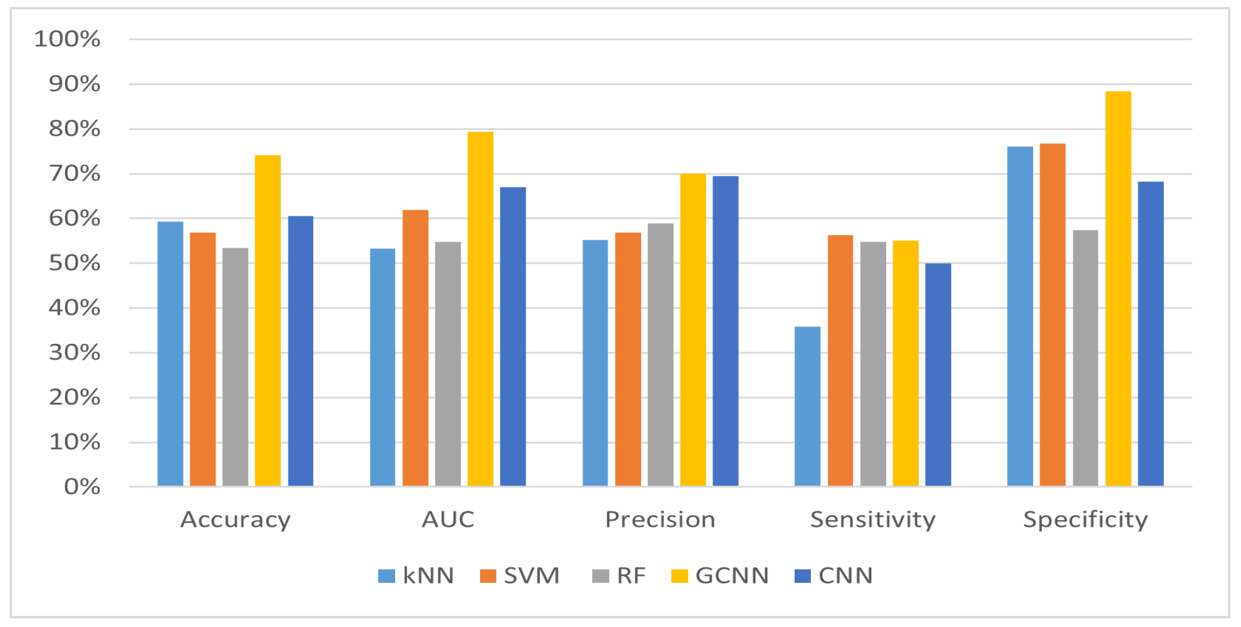
CNN	60.49%	67.03%	69.44%	49.99%	68.19%

. Different performance measures are used to compare each method, such as accuracy, AUC, precision, sensitivity and specificity.

The GCNN outperformed classical methods in all metrics evaluated, demonstrating its effectiveness in predicting stroke risk. With an accuracy of 74.18% and an AUC of 79.32%, the GCNN showed superior performance compared to kNN, SVM and RF, and it also far outperformed the accuracy of the classical CNN method. Moreover, the GCNN demonstrated higher precision, higher sensitivity and competitive specificity, indicating its ability to accurately identify individuals at risk of stroke while minimizing false positives.

6.3. Analysis of Recall and Specificity

In medical scenarios, such as predicting a fatal disease, recall (sensitivity) is particularly important because it measures the ability of the model to correctly identify true positive cases.

The GCNN method achieved the highest recall rate of 84.82%, as shown in Table 2, indicating its superior performance in identifying true positive fatal cases. High sensitivity is of high importance in this type of diagnosis, as it minimizes the proportion of patients in whom a potentially fatal stroke would go unrecognized. Although the GCNN model’s recall is lower in Table 3 (54.98%), it still demonstrates robust performance relative to the other methods, ensuring a balanced trade-off between sensitivity and specificity. In contrast, methods like kNN and SVM also show varying recall rates across the two tables, with kNN achieving a significantly high recall in Table 2 (81.73%) but a lower recall in Table 3 (35.87%). This shows that the performance of the models is strong in different aspects for the two datasets, with one method tending to avoid false negatives and the other tending to minimize false positives.

The specificity values for the prediction of stroke are very high (Figure 4), which means that the model very accurately classifies cases where there is no risk of a stroke within one year. This shows how challenging it is to predict with near certainty that a patient will have a stroke within the next year based on the medical history of the patient during a medical visit. In light of this, further studies will be needed to make our method even more effective.

The outstanding performance of the GCNN compared to classical methods shows that this method can be effectively applied to graph-structured data and can be a useful approach to predicting stroke risk, facilitating preventive screening and improving proactive interventions (see Figure 4 and Figure 5). However, it is important to note that further validation and refinement of the GCNN in a clinical setting are warranted to ensure its accuracy and robustness in everyday patient care.

7. Conclusions

In this work, we have applied a graph-based convolutional neural network deep learning approach to predicting stroke from ICD-10 codes. We have composed our graph representation of the codes based on 57,052 patients and achieved a 74.18% accuracy with a corresponding 79.32% AUC score. To embed the graphs for deep learning purposes, we have applied the PATCHY-SAN strategy. Our comparative analysis has shown that this embedding procedure is superior to other simpler ones, e.g., node2vec. Moreover, our deep convolutional neural network-based approach has outperformed classical machine learning-based techniques, like SVM and Random Forest. To the best of our knowledge, this is the first attempt to predict stroke from ICD-10 codes. However, its accuracy is similar to that of other predictions considering different modalities, which suggests a good possibility of achieving a solid prediction for stroke by combining these results.

8. Discussion

8.1. Graph Embedding Methods

The node2vec method is particularly well suited for mixed-structure data, but with an efficient model, good results can also be obtained for heterophile and structurally identical graphs. We also tried some alternative embedding methods in Python: Deepwalk, LINE and GCN (graph convolutional network). For DeepWalk and LINE, we did not obtain significantly better results compared to node2vec. However, the GCN embedding available in PyTorch showed better results in several cases, performing better in some metrics, although weaker in other metrics. We expect that this will be the subject of further investigation in our future work.

Our results suggest that classical machine learning algorithms do not always provide the best solution for our data. Using node2vec and the GCN in combination, or with further improvements, may be more effective in predicting stroke outcomes. Our future plans include a thorough investigation of different graph embeddings and the development of an ensemble-based method to develop a fusion model that can lead to even more effective predictions. At the same time, we should also consider including other types of patient features in addition to ICD-10 codes and further investigate a more complex dataset.

8.2. Other Deep Learning Methods for Graphs

The aim of our study is to demonstrate the effectiveness of a graph-based deep learning approach in predicting stroke risk and objectively evaluate this performance against traditional methods. We compared our results with traditional machine learning methods (kNN, SVM, Random Forest) because they are widely used and well-established algorithms in predictive modeling, especially in the field of medical data analysis. These methods serve as a baseline and reference point for evaluating the performance of newer methods.

However, in future work, we would like to explore other deep learning methods, such as Graph Attention Networks, GraphSAGE, Graph Recurrent Neural Networks (GRNNs) and Graph Autoencoders.

References

- Nishani, E.; Cico, B. Computer vision approaches based on deep learning and neural networks: Deep neural networks for video analysis of human pose estimation. In Proceedings of the 6th Mediterranean Conference on Embedded Computing (MECO), Bar, Montenegro, 11–15 June 2017; pp. 1–4. [Google Scholar]
- Palaz, D.; Magimai-Doss, M.; Collobert, R. Analysis of CNN-based speech recognition system using raw speech as input. In Proceedings of the InterSpeech, Dresden, Germany, 6–10 September 2015. [Google Scholar]
- Zhu, R.; Zhang, R.; Xue, D. Lesion detection of endoscopy images based on convolutional neural network features. In Proceedings of the International Congress on Image and Signal Processing, Shenyang, China, 14–16 October 2015; pp. 372–376. [Google Scholar]
- Cai, H.; Zheng, V.W.; Chang, K.C. A Comprehensive Survey of Graph Embedding: Problems, Techniques and Applications. IEEE Trans. Knowl. Data Eng. 2018, 30, 1616–1637. [Google Scholar] [CrossRef]
- Kipf, T.; Welling, M. Semi-Supervised Classification with Graph Convolutional Networks. In Proceedings of the International Conference on Learning Representations, Toulon, France, 24–26 April 2017; Available online: https://openreview.net/forum?id=SJU4ayYgl (accessed on 29 April 2024).
- Ahmedt-Aristizabal, D.; Armin, M.A.; Denman, S.; Fookes, C.; Petersson, L. Graph-Based Deep Learning for Medical Diagnosis and Analysis: Past, Present and Future. Sensors 2021, 21, 4758. [Google Scholar] [CrossRef] [PubMed] [PubMed Central]
- Roth, E.J. Hemorrhagic Stroke. In Encyclopedia of Clinical Neuropsychology; Kreutzer, J.S., DeLuca, J., Caplan, B., Eds.; Springer: New York, NY, USA, 2011. [Google Scholar] [CrossRef]
- Lim, G.; Lim, Z.W.; Xu, D.; Ting, D.S.W.; Wong, T.Y.; Lee, M.L.; Hsu, W. Feature Isolation for Hypothesis Testing in Retinal Imaging: An Ischemic Stroke Prediction Case Study. In Proceedings of the Thirty-First AAAI Conference on Innovative Applications of Artificial Intelligence (IAAI-19), Honolulu, HI, USA, 28–30 January 2019. [Google Scholar]
- Cao, Y.; Chi, H.-K.; Khosla, A.; Lin, C.C.Y.; Lee, H.; Hu, J. An integrated machine learning approach to stroke prediction. In Proceedings of the KDD 10, 16th ACM SIGKDD International Conference on Knowledge Discovery and Data Mining, Washington, DC, USA, 25–28 July 2010; pp. 183–192. [Google Scholar]
- Shoily, T.I.; Islam, T.; Jannat, S.; Tanna, S.A.; Alif, T.M.; Ema, R.R. Detection of stroke disease using machine learning algorithms. In Proceedings of the 2019 10th International Conference on Computing, Communication and Networking Technologies (ICCCNT), Kanpur, India, 6–8 July 2019; IEEE: Piscataway, NJ, USA, 2019; pp. 1–6. [Google Scholar]
- Govindarajan, P.; Soundarapandian, R.; Gandomi, A.; Patan, R.; Jayaraman, P.; Manikandan, R. Classification of stroke disease using machine learning algorithms. Neural Comput. Appl. 2019, 32, 817–828. [Google Scholar] [CrossRef]
- Nwosu, C.S.; Dev, S.; Bhardwaj, P.; Veeravalli, B.; John, D. Predicting stroke from electronic health records. In Proceedings of the 2019 41st Annual International Conference of the IEEE Engineering in Medicine and Biology Society (EMBC), Berlin, Germany, 23–27 July 2019; IEEE: Piscataway, NJ, USA, 2019; pp. 5704–5707. [Google Scholar]
- Singh, M.; Choudhary, P. Stroke prediction using artificial intelligence. In Proceedings of the 2017 8th Annual Industrial Automation and Electromechanical Engineering Conference (IEMECON), Bangkok, Thailand, 16–18 August 2017; pp. 158–161. [Google Scholar]
- Jeena, R.; Kumar, S. Stroke prediction using SVM. In Proceedings of the 2016 International Conference on Control, Instrumentation, Communication and Computational Technologies (ICCICCT), Kumaracoil, India, 16–17 December 2016; pp. 600–602. [Google Scholar]
- Parisot, S.; Ktena, S.I.; Ferrante, E.; Lee, M.; Guerrero, R.; Glocker, B.; Rueckert, D. Disease prediction using graph convolutional networks: Application to Autism Spectrum Disorder and Alzheimer’s disease. Med. Image Anal. 2018, 48, 117–130. [Google Scholar] [CrossRef] [PubMed]
- Zhang, S.; Tong, H.; Xu, J.; Maciejewski, R. Graph convolutional networks: A comprehensive review. Comput. Soc. Netw. 2019, 6, 11. [Google Scholar] [CrossRef] [PubMed]
- Palash, G.; Emilio, F. Graph embedding techniques, applications, and performance: A survey. Knowl.-Based Syst. 2018, 151, 78–94. [Google Scholar] [CrossRef]
- Niepert, M.; Ahmed, M.; Kutzkov, K. Learning convolutional neural networks for graphs. In Proceedings of the 33rd International Conference on International Conference on Machine Learning—Volume 48 (ICML’16), New York, NY, USA, 20–22 June 2016; JMLR.org. pp. 2014–2023. [Google Scholar]
- Grover, A.; Leskovec, J. node2vec: Scalable Feature Learning for Networks. KDD 2016, 2016, 855–864. [Google Scholar] [CrossRef] [PubMed] [PubMed Central]
- Scholkopf, B.; Smola, A.J. Support Vector Machines, Regularization, Optimization, and Beyond; MIT Press: Cambridge, MA, USA, 2002; pp. 656–657. [Google Scholar]
- Smola, A.J.; Schölkopf, B. A tutorial on support vector regression. Stat. Comput. 2004, 14, 199–222. [Google Scholar] [CrossRef]
- Guo, G.; Wang, H.; Bell, D.; Bi, Y.; Greer, K. KNN Model-Based Approach in Classification. In On the Move to Meaningful Internet Systems 2003: CoopIS, DOA, and ODBASE. OTM 2003, Catania, Italy, 3–7 November 2003; Meersman, R., Tari, Z., Schmidt, D.C., Eds.; Lecture Notes in Computer Science; Springer: Berlin/Heidelberg, Germany, 2003; Volume 2888. [Google Scholar] [CrossRef]
- Liu, Y.; Wang, Y.; Zhang, J. New Machine Learning Algorithm: Random Forest. In Information Computing and Applications: Third International Conference, ICICA 2012, Chengde, China, 14–16 September 2012; Liu, B., Ma, M., Chang, J., Eds.; Lecture Notes in Computer Science; Springer: Berlin/Heidelberg, Germany, 2012; Volume 7473. [Google Scholar] [CrossRef]