Using Noisy Evaluation to Accelerate Parameter Optimization of Medical Image Segmentation Ensembles

Abstract

An important concern with regard to the ensembles of algorithms is that using the individually optimal parameter settings of the members does not necessarily maximize the performance of the ensemble itself. In this paper, we propose a novel evaluation method for simulated annealing that combines dataset sampling and image downscaling to accelerate the parameter optimization of medical image segmentation ensembles. The scaling levels and sample sizes required to maintain the convergence of the search are theoretically determined by adapting previous results for simulated annealing with imprecise energy measurements. To demonstrate the efficiency of the proposed method, we optimize the parameters of an ensemble for lung segmentation in CT scans. Our experimental results show that the proposed method can maintain the solution quality of the base method with significantly lower runtime. In our problem, optimization with simulated annealing yielded an $F_1$ score of 0.9397 and an associated $MCC$ of 0.7757. Our proposed method maintained the solution quality with an $F_1$ score of 0.9395 and $MCC$ of 0.7755 while exhibiting a 42.01% reduction in runtime. It was also shown that the proposed method is more efficient than simulated annealing with only sampling-based evaluation when the dataset size is below a problem-specific threshold.

1. Introduction

Medical images, along with various omics (e.g., genomics and proteomics) data, now account for the vast majority of data that must be processed and analyzed in healthcare. However, the manual examination of the acquired images is a time-consuming and error-prone process. As a result, as the number of imaging examinations increased, so did the demand for dependable automated methods to assist physicians.

In medical image analysis, image segmentation tasks are critical. For this reason, it is usually not possible to rely on a single algorithm for their clinical implementation. While an algorithm may perform well in general, it may fail in more difficult or uncommon situations. A lesion segmentation algorithm, for example, may perform differently on images acquired with different settings, which is a major issue when images from heterogeneous sources, such as multiple sites, must be processed.

An ensemble of algorithms is commonly considered to address such shortcomings (see, e.g., [1,2,3,4,5,6]). Ensembles are composed of algorithms (members) that use different principles and models to solve a specific problem [7]. The diversity of an ensemble allows it to respond more flexibly to changing conditions [8]. The basic idea behind the ensemble methodology is that by combining the outputs of multiple algorithms with an appropriate aggregation rule [9], a system can be created that outperforms each of its constituent members if certain conditions on their diversity and individual performance are met [10,11].

An important consideration with ensembles is that using the individually optimal parameter setting of the members does not necessarily maximize the ensemble’s performance. For this reason, parameter optimization at the ensemble level is required, which can result in a large-scale problem depending on the number and range of the parameters of the members. Even if the individual members have only a few parameters that can take values from limited ranges, the search space of the possible parameter settings of the ensemble can still be large. Accordingly, an exhaustive search for the optimal parameter setting quickly becomes impractical.

Stochastic search methods are commonly used to solve such large-scale combinatorial optimization problems due to their efficient exploration of solution spaces. These methods can be broadly divided into two main categories: instance-based and model-based.

Instance-based methods rely on iteratively improving the candidate solution through small perturbations and updates. Some notable instance-based methods include Randomized Local Search (RLS) [12], simulated annealing (SA) [13], Genetic Algorithms (GAs) [14,15], and Particle Swarm Optimization (PSO) [16].

RLS is a simple but efficient stochastic search method that explores the neighborhood of the current solution via random sampling. RLS was introduced in the 1950s and is still used today, often as a baseline method. SA is inspired by the annealing process in metallurgy. It improves the solution by exploring the solution space in a controlled manner, starting with more exploration and then transitioning to more exploitation as it progresses. With decreasing probability, it also allows us to accept moves to worse solutions to avoid becoming stuck in local minima. GAs employ natural selection and genetics principles, using populations of candidate solutions and genetic operators, such as mutation and crossover, to explore the search space. PSO is modeled on social behavior, such as bird flocking. Particles in the search space update their positions based on their own best solution and the best solution found by the group. It has been widely applied to various optimization problems.

Model-based methods, in contrast to instance-based approaches, build a probabilistic model of the solution space and use it to guide the search. These methods typically require more computational resources to create and maintain the model. Some popular model-based methods include Ant Colony Optimization (ACO) [17], Cross-Entropy Method (CEM) [18], and Bayesian Optimization (BO) [19].

ACO is an algorithm inspired by the foraging behavior of ants. It uses a population of artificial ants communicating via pheromone trails to find solutions to combinatorial optimization problems. CEM focuses on estimating the distribution of promising solutions and iteratively updating this distribution to generate new candidate solutions. It is known for its capability to handle high-dimensional and complex optimization problems. BO is a powerful technique for optimizing black-box functions, especially in complex optimization scenarios. It uses a probabilistic surrogate model, such as Gaussian processes, to model the objective function and an acquisition function to balance exploration and exploitation. Recently, Bayesian Neural Networks [20], which combine the power of neural networks and Bayesian methods, have become more prevalent for solving optimization problems.

Stochastic approaches can find good solutions to large-scale problems efficiently by sacrificing some accuracy for a significant reduction in search cost. However, even a stochastic search can be very expensive if evaluating a solution is expensive, for example, due to the high complexity of the objective function or the large dataset size, the latter of which is frequently required to avoid parameter overfitting. One approach for reducing the cost of stochastic optimization is to use partial data at each iteration, that is, to approximate the value of the objective function with some noise rather than determining it exactly. The stochastic and mini-batch gradient descent algorithms [21,22], which are widely used in machine learning tasks, rely on a similar principle.

In this paper, we address the parameter optimization problem of image segmentation ensembles by proposing a novel method for the noisy evaluation of the objective function of the metaheuristic SA, which, due to its simplicity and appealing properties, is widely used to solve both discrete and continuous optimization problems.

In a previous study [23], we proposed an evaluation method for SA that uses incremental image resolutions for optimization over image datasets. Naturally, evaluating a solution using lower-resolution images leads to noisy energy values. Our experiments have shown that by using progressively finer image resolutions during the optimization, solutions of the same quality can be found in less time than at the original input resolution, provided that certain conditions regarding the resulting noise are met. In [24], we proposed an evaluation method for SA that is based on the random sampling of the dataset. This method performs evaluations on subsets of appropriate cardinalities of the dataset during the search to maintain the quality of the solution and has been found to be very efficient for large datasets.

Despite the simplicity and efficiency of the image downscaling-based evaluation method, it can be shown that it does not fully exploit the potential of noisy evaluation. It can also be seen that, depending on the problem, image downscaling can introduce noise with a lower standard deviation than dataset sampling with the same cost gain. Based on these observations, here, we investigate the possibility of combining these methods.

The main contributions of this work can be summarized as follows:

• A stochastic approach based on SA is proposed for accelerating parameter optimization of ensembles over image datasets.
• It relies on a novel evaluation method that computes the energy estimate by combining dataset sampling and image downscaling.
• To this end, a strategy is given that can determine the appropriate scaling level and sample size in each search step by adapting convergence results for noisy evaluation in SA.

That is, we have integrated dataset sampling and image downscaling into an evaluation method for SA to leverage their complementary strengths effectively, whose approach extends beyond merely using these two techniques side by side.

The proposed method is primarily intended for optimizing (medical) image segmentation ensembles. To demonstrate the efficiency of the combined noisy evaluation method, we consider optimizing a system comprising an ensemble of conventional image processing algorithms and a post-processing step to segment the lungs in computed tomography (CT) scans. We show that the proposed method reduces the search cost while maintaining the achievable solution’s quality.

The rest of this paper is organized as follows. Section 2 introduces our fundamental concepts and notations, briefly discusses the convergence of SA in the presence of noise, and describes the sampling-based evaluation method that we aim to extend. Then, the proposed evaluation method is described. In Section 3, we present the details of our case study application. Section 4 presents the results of our experiments. We provide detailed results on the efficiency of the three evaluation methods for the parameter optimization of the segmentation ensemble, as well as the performance of the lung segmentation method. Finally, some conclusions are drawn in Section 5.

2. Accelerating SA Using Noisy Evaluation

In this section, we propose a novel evaluation method for SA that combines image downscaling and dataset sampling to reduce the time required for optimization over image datasets. To maintain the convergence of SA in probability, we define a strategy that determines the appropriate scaling level and sample size in each search step by adapting convergence results for noisy evaluation in SA.

2.1. Basic Concepts and Notations

Let $\mathcal{D}=\{D_1,D_2,\dots ,D_M\}$ be an ensemble of $M\in \mathbb{N}$ member algorithms and $\Lambda$ the set of images. The output of the algorithm $D_i$ ($i=1,2,\dots ,M)$ is denoted by $D_i\left(\lambda \right)$ for an image $\lambda \in \Lambda$ and the pixel value of the output at the coordinates $(x,y)$ by $D_i{\left(\lambda \right)}_{(x,y)}$. The output $\mathcal{D}\left(\lambda \right)$ of the ensemble for $\lambda$ is determined by applying an aggregation rule to the individual outputs of the algorithms $D_1,D_2,\dots ,D_M$.

Different parameter settings can be considered for the member algorithms. Let ${\Pi }_i$ denote the J-dimensional parameter space and ${\pi }_i=({\pi }_{i,1},{\pi }_{i,2},\dots ,{\pi }_{i,J})\in {\Pi }_i$ a given parameter setting of the algorithm $D_i$$(i=1,2,\dots ,M)$. Furthermore, let $\pi \in \Pi ={\Pi }_1\times {\Pi }_2\times \dots \times {\Pi }_M$ denote a given parameter setting of the ensemble. Then, the ensemble with a specific parameter setting $\pi$ is denoted by ${\mathcal{D}}^{\left(\pi \right)}$.

In our application, $\lambda \in {\Lambda }_N\subset \Lambda$, where ${\Lambda }_N$ is a set of $N\in \mathbb{N}$ images, and the ensemble members are image segmentation algorithms, whose outputs are aggregated using majority voting.

2.2. Convergence of SA in Presence of Noise

SA is a local search algorithm inspired by the metallurgical annealing process, and it was developed to address difficult combinatorial optimization problems. The main feature of SA is its ability to escape from local optima by accepting non-improving moves with a probability determined by the objective function (energy) difference between the current and candidate states and a decreasing control parameter (temperature) generated by a cooling schedule.

SA was designed with the assumption that the energy of a state can be calculated exactly, but in practice, the evaluation of a state is often subject to noise. This noise can be given as the difference of the energy E and its noisy estimate $\widehat{E}$, i.e., as

$$d=\widehat{E}-E.$$

(1)

Let us consider a discrete search space and assume that the noise in the k-th ($k\in \mathbb{N}$) iteration is normally distributed with mean 0 and variance ${\left({\sigma }_d^{\left(k\right)}\right)}^2>0$. Gelfand and Mitter proved [25] that SA converges to the global optimum in probability using noisy evaluation in the same manner as using exact energy values if the standard deviation ${\sigma }_d^{\left(k\right)}$ of the noise in the k-th iteration for each k is dominated by the temperature $T^{\left(k\right)}$, i.e., when

$${\sigma }_d^{\left(k\right)}=o\left(T^{\left(k\right)}\right).$$

(2)

To ensure the convergence of SA with noisy evaluation, we have to control the standard deviation of the noise during the search according to (2). Therefore, for each k, we need to determine the maximum allowed value $s^{\left(k\right)}$ for the standard deviation ${\sigma }_d^{\left(k\right)}$ of the noise with respect to the temperature $T^{\left(k\right)}$. For this, we can apply Lemma 1 from our previous work [24] as

$$s^{\left(k\right)}\approx T^{\left(k\right)}{(1-ϵ)}^k,0<ϵ\ll 1.$$

(3)

2.3. SA with Sampling-Based Evaluation (SA-SBE)

In [24], we proposed a sampling-based evaluation method for SA to accelerate optimization over large datasets. For the evaluation of a state, the proposed method considers only the minimum part of the dataset required to maintain the quality of the solution in each iteration. We have shown that using this method significantly reduces the time required for optimization compared to using standard SA without compromising the achievable solution quality.

The main result of [24] and the basis of the SA-SBE evaluation method is that for an arbitrary cooling schedule, the minimum sample size $n^{\left(k\right)}$ required at the k-th iteration to maintain the convergence of the method in probability can be estimated as

$$n^{\left(k\right)}\approx \frac{N{\sigma }_{max}^2}{(N-1){s^{\left(k\right)}}^2+{\sigma }_{max}^2},$$

(4)

where N is the size of the dataset, ${\sigma }_{max}$ is the worst-case maximum value of the standard deviation of the evaluation metric over the images of the dataset, and $s^{\left(k\right)}$ can be approximated using (3).

2.4. Improving SA-SBE with Image Downscaling

In this section, we present an evaluation method that combines dataset sampling and image downscaling to further accelerate optimization with SA over image datasets. This method is based on the observation that, depending on the problem, downscaling with the same cost gain can introduce noise with a lower standard deviation than dataset sampling.

2.4.1. Image Pyramid Representation

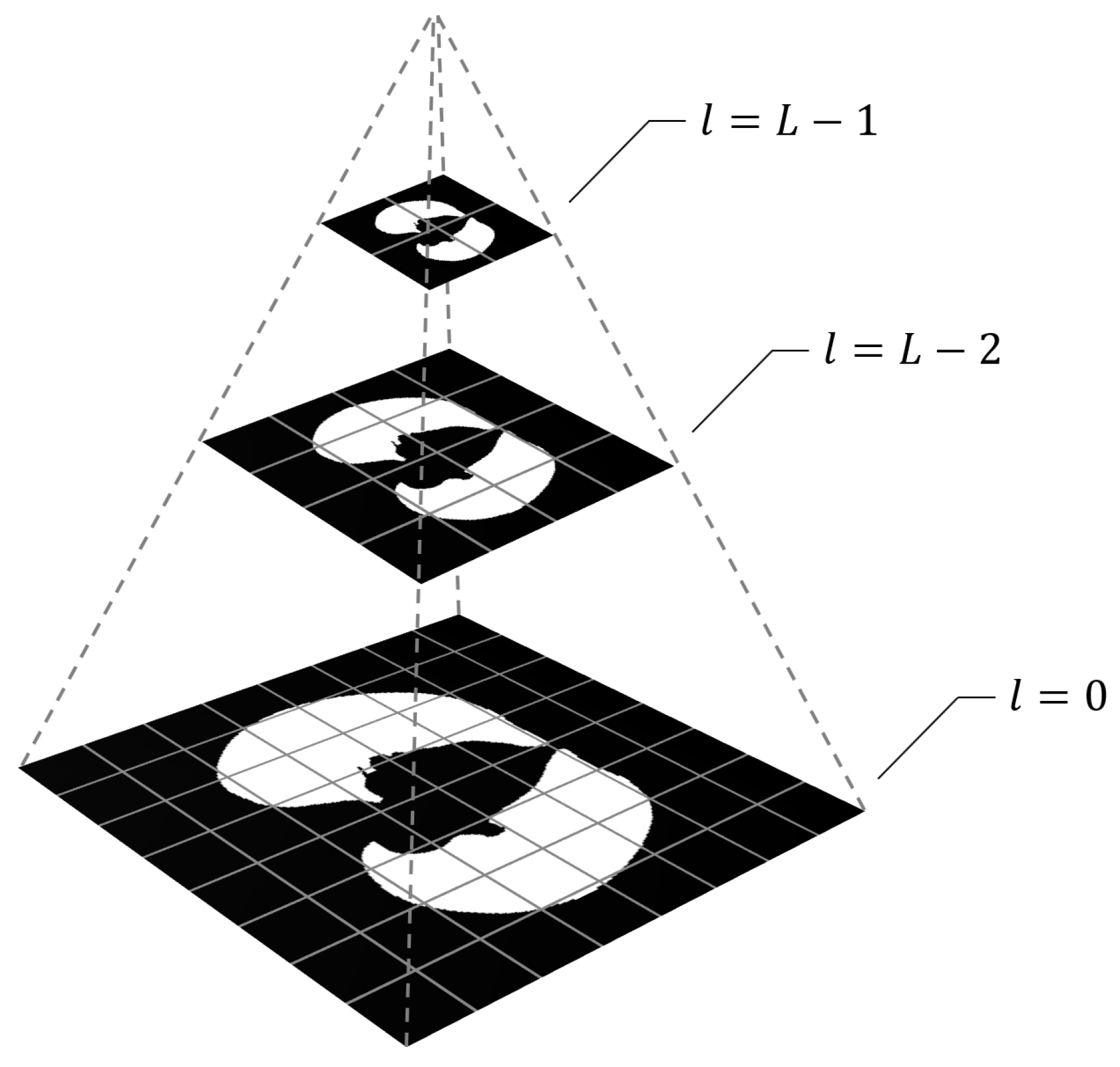
To implement downscaling, a pyramid representation of the dataset images is considered. An image pyramid is a collection of images derived from a single original that are successively downscaled until a termination criterion (e.g., a desired minimum resolution) is not met.

The most common technique for creating pyramid representations of images is the Gaussian pyramid [26], in which each level is constructed by convolving the original image with a Gaussian-like averaging filter before subsampling. Note that in the case of the optimization problems we consider, the ground truth corresponding to the input images are binary masks. Therefore, when creating the pyramid representations of the ground truth images, we skip the Gaussian filtering step in order to preserve the sharp boundaries. That is, the pixel values of a level are defined to match the pixel whose center is closest to the sampling position in the original image.

Specifically, we will refer to a collection of $L\in \mathbb{N}$ hierarchically downscaled versions of an image as an L-level image pyramid, in which the higher the scaling level l ($l\in 0,1,\cdots ,L-1$), the lower the image resolution. The original image is at $l=0$, and each level $l>0$ is scaled down by a factor of $2^l$. For a visual explanation of this construction, see Figure 1.

2.4.2. Effects of Downscaling

Naturally, using downscaled versions of the dataset images accelerates the evaluation. Assuming that the cost of calculating the energy E is proportional to the resolution of the input images, calculating the energy estimate ${\widehat{E}}_l$ using the scaling level l results in a cost that is $1/2^l$ times lower. Using a scaling level $l>0$, on the other hand, introduces an additional energy noise $d_l$, which is determined as

$$d_l={\widehat{E}}_l-E.$$

(5)

To establish the proposed evaluation method, we need to determine both the standard deviation of the noise ${\sigma }_{d_l}$ caused by downscaling and the evaluation cost $c_l$ of an image for each scaling level l of the image pyramid.

It should be noted that the amount of noise can vary significantly for different energy functions when downscaled versions of the images from the dataset are used for the evaluation. In some cases, determining the theoretical maximum value of ${\sigma }_{d_l}$ for a given level l may be straightforward, but for more complex energy functions, it becomes a difficult problem. Furthermore, in the case of natural images, the empirical standard deviation of the noise for a level l is likely to be much lower than the theoretical maximum. Therefore, even if the theoretical maximum noise standard deviation can be determined, we propose estimating both ${\sigma }_{d_l}$ and $c_l$ for each level l of the image pyramid by measuring these values over the ground truth used for evaluation.

2.4.3. Combining Dataset Sampling and Image Downscaling

When combining dataset sampling and image downscaling, we have to deal with a noise that is the sum of noises originating from the dataset sampling $d_n$ and the image downscaling $d_l$. Since $d_n$ and $d_l$ are uncorrelated, the standard deviation of the sum of these noises ${\sigma }_{(d_n+d_l)}$ can be calculated as the square root of the sum of their variances, that is, as

$${\sigma }_{(d_n+d_l)}=\sqrt{{\sigma }_{d_n}^2+{\sigma }_{d_l}^2}.$$

(6)

Furthermore, to maintain the convergence of the search,

$${\sigma }_{(d_n+d_l)}^{\left(k\right)}\le s^{\left(k\right)}$$

(7)

must hold in each iteration k.

Our goal is to minimize the total cost of the search, e.g., in terms of computation time. To accomplish this, we need to find the scaling level l and sample size n, whose combination will minimize the cost $C_{l,n}^{\left(k\right)}$ in each iteration k, while ensuring that (7) holds. For this, the following method can be used:

• Estimate ${\sigma }_{d_l}$ and $c_l$ for each level l of the image pyramid using the ground truth (for a concrete realization; see Section 4.4).
• For each scaling level l whose corresponding noise standard deviation ${\sigma }_{d_l}\le s^{\left(k\right)}$, estimate the minimum required sample size n by adapting (4) as

  $$n\approx \frac{N{\sigma }_{max}^2}{(N-1)\sqrt{{s^{\left(k\right)}}^2-{\sigma }_{d_l}^2}+{\sigma }_{max}^2}.$$

  (8)
• Calculate the corresponding cost $C_{l,n}^{\left(k\right)}=n{c}_l$.
• Finally, choose the combination of l and n, for which $C_{l,n}^{\left(k\right)}$ is minimal.

Note that this method guarantees that the scaling level l decreases monotonically during the search if the corresponding noise standard deviation $d_l$ decreases monotonically, which is a natural assumption. Thus, we propose not calculating the cost for scaling levels higher than the one used in the previous iteration.

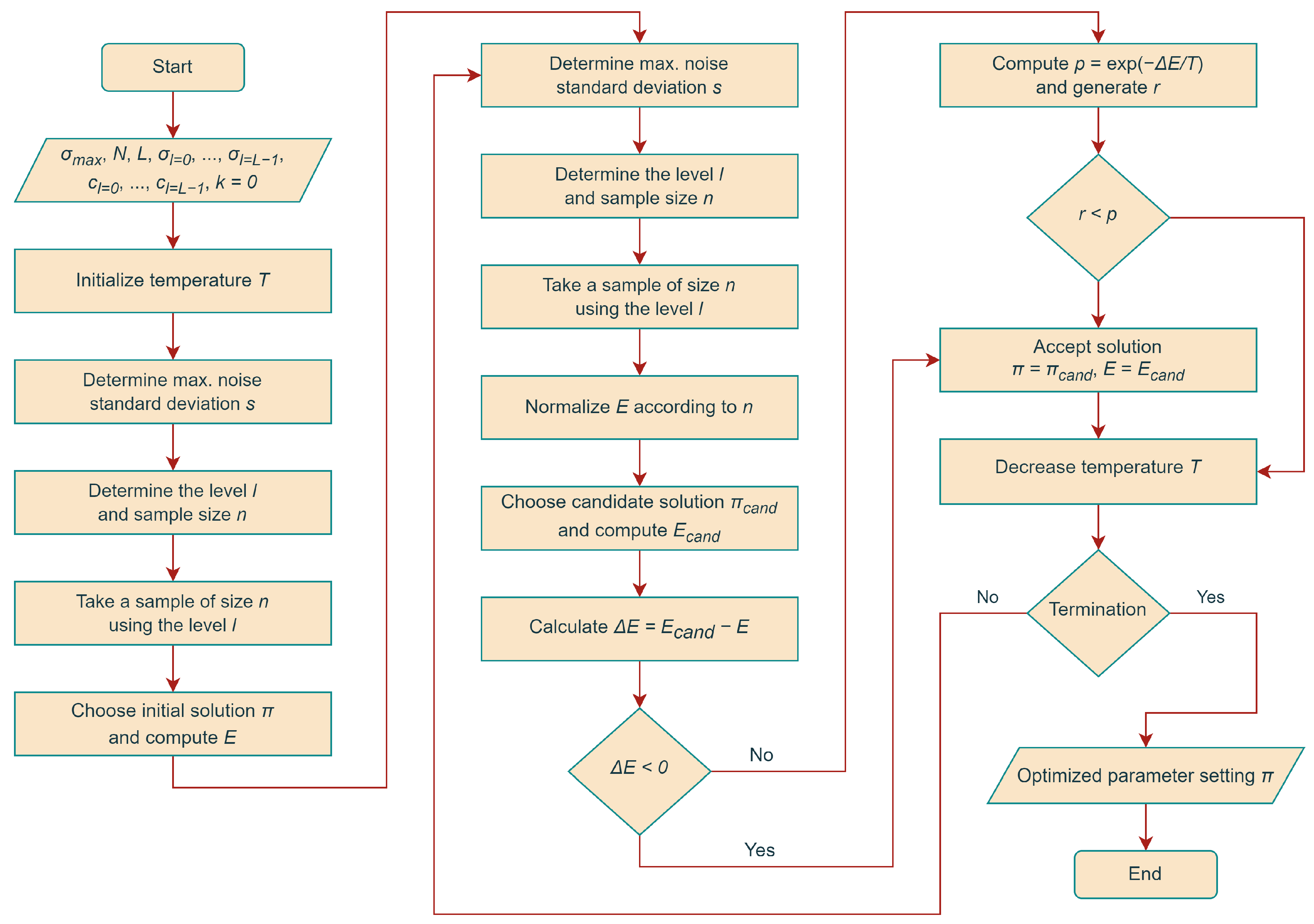
Hereafter, we refer to SA using the above strategy to compute energy estimates during the search as SA with Combined Noisy Evaluation (SA-CNE). See Figure 2 for a visual explanation of the proposed method.

2.5. Example

As a numerical demonstration of the total cost of the method described above, let us consider a problem with a maximum standard deviation of the evaluation metric ${\sigma }_{max}=0.5$ and a training set size $N=200$. For the image pyramid, let us use $L=5$ levels with the corresponding noise standard deviations ${\sigma }_{d_{l=0}}=0.0$, ${\sigma }_{d_{l=1}}=0.02$, ${\sigma }_{d_{l=2}}=0.05$, ${\sigma }_{d_{l=3}}=0.09$, and ${\sigma }_{d_{l=4}}=0.15$, and the corresponding evaluation costs $c_l=\frac{1}{2^{2l}}$ ($l\in \{1,2,\cdots ,L-1\}$). Furthermore, let us use an exponential cooling schedule in SA with

$$T^{\left(k\right)}=T^{\left(0\right)}{\alpha }^k,$$

(9)

where $T^{\left(0\right)}=5$, $\alpha =0.99$, and $0\le k<1000$.

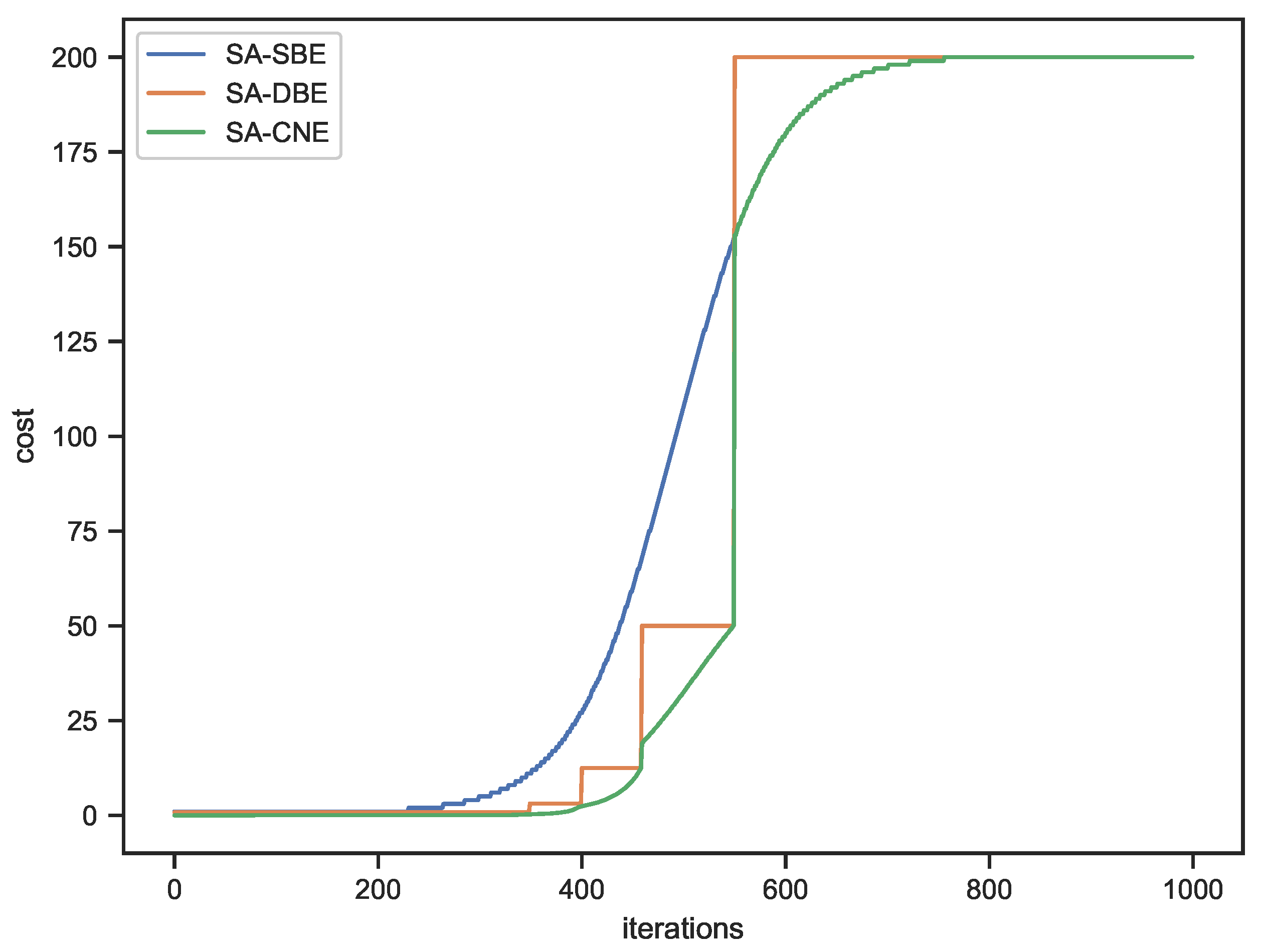
For this setup, the total theoretical cost of optimization is 200,000 when using standard SA, 101,905 when using dataset sampling (SA-SBE), 95,719.5 when using downscaling-based evaluation (SA-DBE), and 90,902.5 when combining dataset sampling and image downscaling (SA-CNE). The change in cost during optimization for both methods are shown in Figure 3.

The behavior of the three curves in Figure 3 can be described as follows:

• The SA-SBE curve shows a smooth but marked increase in cost as the optimization progresses due to the exponential cooling schedule used. It indicates that SA-SBE is significantly more computationally efficient at higher temperatures, i.e., when smaller sample sizes can be used. As the optimization approaches the end, the evaluation cost becomes similar to that of SA due to the larger sample sizes required.
• The SA-DBE curve is characterized by a stair-like pattern, where the cost remains constant while using the same pyramid level. Then, there is a sharp increase in cost when the method switches to a lower (higher resolution) level of the image pyramid, which is required to stay below the maximum allowable noise standard deviation. In this example, the SA-DBE curve remains below the SA-SBE curve for most of the optimization process, indicating that the use of image downscaling introduces a lower noise standard deviation, e.g., using images downscaled with a factor of 0.5 in each dimension introduces a lower noise standard deviation than using 25% of the dataset, which results in lower overall evaluation costs compared to SA-SBE.
• The SA-CNE curve also shows a step-like pattern, but the connecting sections between the steps resemble a section of the SA-SBE curve. It reflects the combined strategy of dataset sampling and image downscaling. The sharp steps denote switching to a lower level in the image pyramid, while the connecting curve segments indicate the increasing sample sizes at the same level.

Overall, SA-CNE exhibits lower evaluation costs than both SA-SBE and SA with image downscaling, highlighting its computational efficiency while maintaining solution quality. It can also be observed that the curve of SA-CNE transitions into the curve of SA-SBE when the lowest level of the pyramid (i.e., the original image size) is used. The curve of SA is not shown in Figure 3, as it maintains a constant evaluation cost regardless of the optimization progress, using the entire dataset at its original resolution in each search step.

3. Application: Lung Segmentation in CT Scans

CT scans are commonly used in computer-aided diagnosis systems to detect and characterize various lung abnormalities. Lung segmentation is a key step in these systems that can significantly affect their performance.

Several methods for lung segmentation have been proposed over the last two decades. Conventional methods rely on techniques such as thresholding [27,28], region growing [29,30], active contours [31,32], mathematical morphology [33,34], and cluster analysis [35,36,37]; however, deep learning (DL) approaches, in particular convolutional neural networks [38,39], generative adversarial networks [40,41], and residual neural networks [42], have recently gained popularity in this field as well. While DL methods achieve state-of-the-art accuracy, a drawback of these methods is that they require substantial amounts of annotated training data to achieve the desired accuracy.

Another approach to improve accuracy is to create an ensemble of segmentation methods by merging their output using an aggregation rule [10]. The rest of this section describes our case study application, which segments the lungs using an ensemble of conventional segmentation methods and a post-processing step.

3.1. The Segmentation Ensemble

Next, we describe the members of the lung segmentation ensemble and the aggregation method used to combine their outputs.

3.1.1. Member Algorithms

Our lung segmentation ensemble consists of three simple, conventional image processing algorithms, each of which works on the slices of the CT scans. These methods have been developed to have different operating principles to increase the diversity of the ensemble, i.e., the independence of the outputs of the members, and thus to reduce the segmentation error. No common pre-processing techniques are used for the ensemble members. Each algorithm includes all the steps required to generate a binary lung mask for the input slices.

Algorithm $D_1$: This algorithm is based on connected component analysis. First, the input image is thresholded to estimate an initial lung mask; then, the connected components in the resulting binary image are labeled. Those components that are touching the border of the image are removed, and the two largest remaining components are kept as lung candidates. After this, morphological erosion is performed to separate the lung nodules attached to the blood vessels, and morphological closing is used to retain nodules attached to the lung wall. Finally, the holes inside the binary mask of the lungs are filled. $D_1$ has the following parameters: the threshold to gain the initial lung mask ${\pi }_{1,1}$; the radius of the disk structuring element (SE) for erosion ${\pi }_{1,2}$; and the radius of the disk SE for closing ${\pi }_{1,3}$.

Algorithm $D_2$: This algorithm is based on k-means clustering. First, the image is standardized to have pixel values with mean 0 and standard deviation 1. After this, k-means clustering is used to partition the image into $k=2$ clusters, representing lungs/air and tissues/bones. The resulting binary image is then refined using morphological erosion and a subsequent dilation using a larger SE in order to avoid missing lung pixels. Then, the air outside the body of the subject and those objects that are too small to be lungs (less than 1% of the image area) are removed. Finally, morphological closing is performed to fill small holes. $D_2$ has the following parameters: the radius of the disk SEs for erosion ${\pi }_{2,1}$; for dilation ${\pi }_{2,2}$; and for closing ${\pi }_{2,3}$.

Algorithm $D_3$: This algorithm is based on contour detection. First, the intensity values of the input image are clipped to an interval that roughly represents lungs/air. That is, intensities below the minimum and above the maximum of the interval are set to these values, respectively. Then, the image is binarized, and its contours are detected using the “marching squares” method for a given level. After this, non-closed contours are removed. Using a minimum area (the square root of the image area) and a maximum area (the quarter of the image area), unwanted small contours and the contour of the body are removed. The remaining contours are assumed to correspond to the lungs. Finally, a lung mask is created, converting the list of the remaining contours to a binary image. $D_3$ has the following parameters: the minimum ${\pi }_{3,1}$ and maximum ${\pi }_{3,2}$ values of the interval for clipping, and the level ${\pi }_{3,3}$ for contour detection.

In

Table 1. Adjustable parameters of the ensemble members.

Alg.	Parameter Description	Range
$D_1$	initial mask threshold	${\pi }_{1,1}\in \{-450,-400,-350\}$
$D_1$	erosion SE radius	${\pi }_{1,2}\in \{1,2,3\}$
$D_1$	closing SE radius	${\pi }_{1,3}\in \{8,9,10,11,12\}$
$D_2$	erosion SE radius	${\pi }_{2,1}\in \{1,2,3\}$
$D_2$	dilation SE radius	${\pi }_{2,2}\in \{3,4,5\}$
$D_2$	closing SE radius	${\pi }_{2,3}\in \{1,2,3\}$
$D_3$	interval minimum	${\pi }_{3,1}\in \{-1050,-1000,-950\}$
$D_3$	interval maximum	${\pi }_{3,2}\in \{-450,-400,-350\}$
$D_3$	contour level	${\pi }_{3,3}\in \{0.75,0.85,0.95\}$

, we summarize the adjustable parameters of the ensemble members. Overall, there are $3^8\times 5$ = 32,805 possible different parameter settings for the ensemble.

3.1.2. Aggregation Method

We use pixel-level majority voting to aggregate the individual member outputs in order to obtain the output of the ensemble. That is, the pixel values of the ensemble output ${\mathcal{D}}^{\left(\pi \right)}\left(\lambda \right)$ for the image $\lambda$ using the parameter setting $\pi$ is determined as

$${\left({\mathcal{D}}^{\left(\pi \right)}\left(\lambda \right)\right)}_{(x,y)}=\left\{\begin{array}{c}1,\mathrm{if}\sum _{i=1}^M{\left(D_i^{\left(\pi \right)}\left(\lambda \right)\right)}_{(x,y)}>\left[\frac{M}{2}\right],\hfill \\ 0,\mathrm{otherwise},\hfill \end{array}\right.$$

(10)

where M = 3 is the number of member algorithms and $(x,y)$ are the pixel coordinates.

3.2. Post-Processing: Removing Air Pockets

The previously presented ensemble performs lung segmentation at the CT slice level. However, after aggregating the segmentation outputs of the members and building a new volume from these consensus slices, the result can be improved by removing the small air pockets and keeping only those that are almost certainly lung.

For this, we use the following simple method: First, the connected components of the volume are labeled, and the voxel count for each unique label is calculated. In addition, the background is removed in this step. Then, if there are still at least two connected components, we check whether the largest component has at least twice the voxel count of the second-largest one. If it holds, the largest component is retained; we assume that the lungs and trachea are not separated. If this condition does not hold, we assume that the lungs and trachea have been separated and keep the two largest components. If only one label remains after removing the background, that component is considered as lung.

4. Experimental Results

In this section, we present the methods and results of our experiments. We start by describing the dataset used, followed by a discussion of the methodology applied to evaluate the proposed optimization methods. We then present the results of our experiments. Finally, we provide the implementation details.

4.1. Dataset

Parameter optimization of the ensemble was performed using the publicly available COVID-19 CT Lung and Infection Segmentation Dataset [43]. This dataset consists of 20 thoracic CT scans and corresponding annotations, both stored in NIfTI (Neuroimaging Informatics Technology Initiative) format. The CT scans were provided by the Coronacases Initiative [44] and Radiopaedia [45]. The left and right lungs and signs of COVID-19 infection were labeled by two radiologists and reviewed by a third experienced radiologist. The 10 CT scans provided by the Coronacases Initiative were used for the experiments from this dataset. The resolution of these CT scans ranges from $512\times 512\times 200$ to $512\times 512\times 301$ pixels, and they contain a total of 2581 slices.

In our experiments, we used 10 training sets, each created from the dataset described above as follows: first, we randomly selected three of the ten CT scans; then, we randomly selected 100 slices from each of these scans. In this way, we obtained training sets of 300 slices each. The remaining seven CT scans were used as the corresponding test set for each training set.

4.2. Evaluation Methodology

We performed parameter optimization of the ensemble presented in Section 3 to assess the efficiency of the proposed stochastic search method.

We considered each CT slice as a separate image $\lambda$ for the evaluation. The ensemble output ${\mathcal{D}}^{\left(\pi \right)}\left(\lambda \right)$ for the image $\lambda$ using the parameter setting $\pi$ was compared with the corresponding binary ground truth mask $\tau$. That is, a pixel was considered a true positive if it was correctly classified as foreground; otherwise, it was considered a false positive. In addition, an unrecognized foreground pixel was treated as a false negative, while a correctly classified background pixel was treated as a true negative. For the i-th image ${\lambda }_{i,l}$ scaled to the l-th image pyramid level, we denote the number of true positives as $T{P}_{{\lambda }_{i,l}}$, the number of false positive as $F{P}_{{\lambda }_{i,l}}$, the number of false negatives as $F{N}_{{\lambda }_{i,l}}$, and the numbers of true negatives as $T{N}_{{\lambda }_{i,l}}$. If $l=0$, we use the short notations $T{P}_{{\lambda }_i}$, $T{N}_{{\lambda }_i}$, $F{P}_{{\lambda }_i}$, and $F{N}_{{\lambda }_i}$, respectively.

The goal of the optimization was to find the parameter setting that maximizes the segmentation performance of the ensemble in terms of the mean $F_1$ score. Specifically, for a given level l of the image pyramid and for a set of n images, we computed the mean $F_1$ score ${\overline{F_1}}_{l,n}$ for each $l=0,1,\cdots ,L-1$ as follows:

$${\overline{F_1}}_{l,n}=\frac{1}{n}\sum _{i=1}^n\frac{2T{P}_{{\lambda }_{i,l}}}{2T{P}_{{\lambda }_{i,l}}+F{P}_{{\lambda }_{i,l}}+F{N}_{{\lambda }_{i,l}}},$$

(11)

where ${\lambda }_{i,l}$ is the i-th image downscaled to the image pyramid level l, L is the number of levels in the image pyramid, and n is the number of images used. In the case $l=0$ and $n=N$, we use the short notation $\overline{F_1}$.

Furthermore, for a solution, we calculated the mean Matthews correlation coefficient $\overline{MCC}$, the mean accuracy $\overline{ACC}$, the mean sensitivity $\overline{SE}$, and the mean specificity $\overline{SP}$ measures as:

$$\overline{MCC}=\frac{1}{N}\sum _{i=1}^N\frac{T{P}_{{\lambda }_i}T{N}_{{\lambda }_i}-F{P}_{{\lambda }_i}F{N}_{{\lambda }_i}}{{\left((T{P}_{{\lambda }_i}+F{P}_{{\lambda }_i})(T{P}_{{\lambda }_i}+F{N}_{{\lambda }_i})(T{N}_{{\lambda }_i}+F{P}_{{\lambda }_i})(T{N}_{{\lambda }_i}+F{N}_{{\lambda }_i})\right)}^{\frac{1}{2}}},$$

(12)

$$\overline{ACC}=\frac{1}{N}\sum _{i=1}^N\frac{T{P}_{{\lambda }_i}+T{N}_{{\lambda }_i}}{T{P}_{{\lambda }_i}+T{N}_{{\lambda }_i}+F{P}_{{\lambda }_i}+F{N}_{{\lambda }_i}},$$

(13)

$$\overline{SE}=\frac{1}{N}\sum _{i=1}^N\frac{T{P}_{{\lambda }_i}}{T{P}_{{\lambda }_i}+F{N}_{{\lambda }_i}},$$

(14)

$$\overline{SP}=\frac{1}{N}\sum _{i=1}^N\frac{T{N}_{{\lambda }_i}}{T{N}_{{\lambda }_i}+F{P}_{{\lambda }_i}}.$$

(15)

4.3. Design Choices

A number of design decisions need to be made in order to implement the proposed stochastic search method. It is necessary to determine the initial state, the neighborhood function, the acceptance criterion, the cooling schedule, the termination criterion, the energy function, and the number of levels in the image pyramid. Some of the design decisions are as follows:

• Pyramid levels: The number of image pyramid levels was set to $L=5$.
• Cooling schedule: We chose the exponential cooling schedule defined in (9), of which the initial temperature $T^{\left(0\right)}=1$ and $\alpha =0.985$ were set.
• Energy function: To obtain a minimization problem, we defined the energy function as

  $$E=1-\overline{F_1},$$

  (16)

  and the energy function estimate for the level l and a set of n images as

  $${\widehat{E}}_{l,n}=1-{\overline{F_1}}_{l,n}.$$

  (17)
• Termination criterion: We chose a fixed number of iterations with $0\le k<500$.

The remaining design decisions were made according to the description in [24].

4.4. Estimation of the Noise and Cost Gain Caused by Downscaling

To estimate the noise caused by evaluating the segmentation performance of the ensemble using downscaled versions of the dataset images, we measured the noise using the corresponding ground truth masks provided with the dataset (i.e., the noise in the case of perfect segmentation) for each level $l=0,1,\cdots ,L-1$ as follows:

• First, for a level l and for each ground truth mask ${\tau }_i$ ($i=1,\cdots ,N$), we generated the images ${\tau }_{i,l}$ by scaling them down by the factor ${\gamma }_l=1/2^l$.
• The images ${\tau }_{i,l}$ were then scaled up to their original size to obtain ${\tau }_{i,l}^{{}^{\prime }}$.
• Then, for each ground truth mask ${\tau }_i$, we calculated the noise $d_{i,l}$ as the difference of the energy estimate and the energy, considering perfect segmentation, i.e., as

  $$d_{i,l}=\frac{2T{P}_{{\tau }_{i,l}^{{}^{\prime }}}}{2T{P}_{{\tau }_{i,l}^{{}^{\prime }}}+F{P}_{{\tau }_{i,l}^{{}^{\prime }}}+F{N}_{{\tau }_{i,l}^{{}^{\prime }}}}-1.$$

  (18)
• Finally, we estimated ${\sigma }_{d_l}$ by calculating the standard deviation of the noises $d_{i,l}$. Also, to estimate $c_l$, we measured the average cost (time) required to calculate the energy for an image ${\tau }_{i,l}$.

4.5. Optimization Results

The main results obtained in our experiments regarding the efficiency of the proposed optimization method are summarized in

Table 2. Results of the parameter optimization using the 10 training sets.

Method	$\overline{{\mathit{F}}_1}$	$\overline{\mathit{MCC}}$	$\overline{\mathit{ACC}}$	$\overline{\mathit{SE}}$	$\overline{\mathit{SP}}$	t (s)
Exhaustive search	0.7956 (±0.0377)	0.7737 (±0.0356)	0.9927 (±0.0015)	0.9367 (±0.0145)	0.9960 (±0.0005)	4465.8 (±25.3)
SA	0.7954 (±0.0377)	0.7735 (±0.0356)	0.9927 (±0.0015)	0.9378 (±0.0145)	0.9959 (±0.0006)	67.6 (±0.4)
SA-SBE	0.7953 (±0.0377)	0.7735 (±0.0356)	0.9927 (±0.0015)	0.9369 (±0.0148)	0.9960 (±0.0005)	45.6 (±0.5)
SA downscaling	0.7954 (±0.0378)	0.7735 (±0.0356)	0.9926 (±0.0015)	0.9363 (±0.0148)	0.9960 (±0.0005)	44.9 (±0.3)
SA-CNE	0.7955 (±0.0378)	0.7736 (±0.0356)	0.9927 (±0.0015)	0.9370 (±0.0143)	0.9960 (±0.0006)	39.2 (±0.3)

. Here, we present the $\overline{F_1}$, $\overline{MCC}$, $\overline{ACC}$, $\overline{SE}$, and $\overline{SP}$ values, as well as the average runtimes t (in seconds) and the corresponding standard deviations calculated based on the results obtained using the 10 training sets. The optimization was repeated three times for each method and training set, and the run with the best energy function value was selected. The results for the solutions found with a brute-force search (i.e., the achievable maximum performance) is also included for reference.

Table 2 shows that both the sampling-based and the downscaling-based, as well as the two methods combined, maintained the solution quality of the standard SA, but required significantly less time (−32.54%, −33.58%, and −42.01%, respectively). That is, the $\overline{F_1}$ values obtained with these three optimization methods were only marginally different from those obtained with the standard SA. It is also shown that the combined method could further speed up the optimization process without compromising solution quality. Furthermore, all methods exhibited consistent behavior in terms of the standard deviations of the evaluation measures.

For a comprehensive illustration of the optimization process, see the Supplementary Materials, which contains the energy curves of the SA-CNE method corresponding to the test datasets.

4.6. Lung Segmentation Results

For each parameter setting obtained using the training sets, we used the corresponding test sets for evaluation as follows. First, we evaluated the performance of the lung segmentation ensemble without the air pocket removal (post-processing) step. That is, we processed all slices of the CT scans in the test sets using the segmentation ensemble to obtain the mean metrics for each test set. Then, these values were averaged over the 10 test sets. The corresponding results can be found in

Table 3. Lung segmentation performance without post-processing.

Method	$\overline{{\mathit{F}}_1}$	$\overline{\mathit{MCC}}$	$\overline{\mathit{ACC}}$	$\overline{\mathit{SE}}$	$\overline{\mathit{SP}}$
Exhaustive search	0.7742 (±0.0159)	0.7593 (±0.0177)	0.9919 (±0.0007)	0.9314 (±0.0096)	0.9957 (±0.0004)
SA	0.7745 (±0.0157)	0.7596 (±0.0175)	0.9920 (±0.0007)	0.9322 (±0.0091)	0.9957 (±0.0003)
SA-SBE	0.7744 (±0.0157)	0.7595 (±0.0174)	0.9920 (±0.0007)	0.9316 (±0.0090)	0.9957 (±0.0003)
SA downscaling	0.7741 (±0.0158)	0.7592 (±0.0177)	0.9919 (±0.0007)	0.9309 (±0.0104)	0.9958 (±0.0004)
SA-CNE	0.7744 (±0.0158)	0.7595 (±0.0176)	0.9920 (±0.0007)	0.9318 (±0.0095)	0.9957 (±0.0003)

.

Next, we evaluated the lung segmentation performance using the volume-level air pocket removal method to improve the final segmentation performance. To accomplish this, we generated a new volume from the output of the segmentation ensemble for a given CT scan and applied the air pocket removal method to it. For comparison, the CT scans of the test sets were also processed using the state-of-the-art DL method U-Net trained on a dataset of 231 CT scans [38]. In both cases, we calculated the mean metrics at the slice level. See

Table 4. Lung segmentation performance with post-processing.

Method	$\overline{{\mathit{F}}_1}$	$\overline{\mathit{MCC}}$	$\overline{\mathit{ACC}}$	$\overline{\mathit{SE}}$	$\overline{\mathit{SP}}$
Exhaustive search	0.9393 (±0.0066)	0.7753 (±0.0178)	0.9939 (±0.0006)	0.9311 (±0.0097)	0.9978 (±0.0004)
SA	0.9397 (±0.0068)	0.7757 (±0.0175)	0.9939 (±0.0006)	0.9319 (±0.0092)	0.9977 (±0.0003)
SA-SBE	0.9395 (±0.0068)	0.7754 (±0.0175)	0.9939 (±0.0006)	0.9314 (±0.0091)	0.9978 (±0.0003)
SA downscaling	0.9391 (±0.0071)	0.7750 (±0.0180)	0.9939 (±0.0006)	0.9306 (±0.0104)	0.9978 (±0.0003)
SA-CNE	0.9395 (±0.0067)	0.7755 (±0.0175)	0.9939 (±0.0006)	0.9315 (±0.0095)	0.9977 (±0.0003)
U-Net (R-231) [38]	0.9651 (±0.0023)	0.8015 (±0.0155)	0.9968 (±0.0002)	0.9693 (±0.0021)	0.9979 (±0.0002)

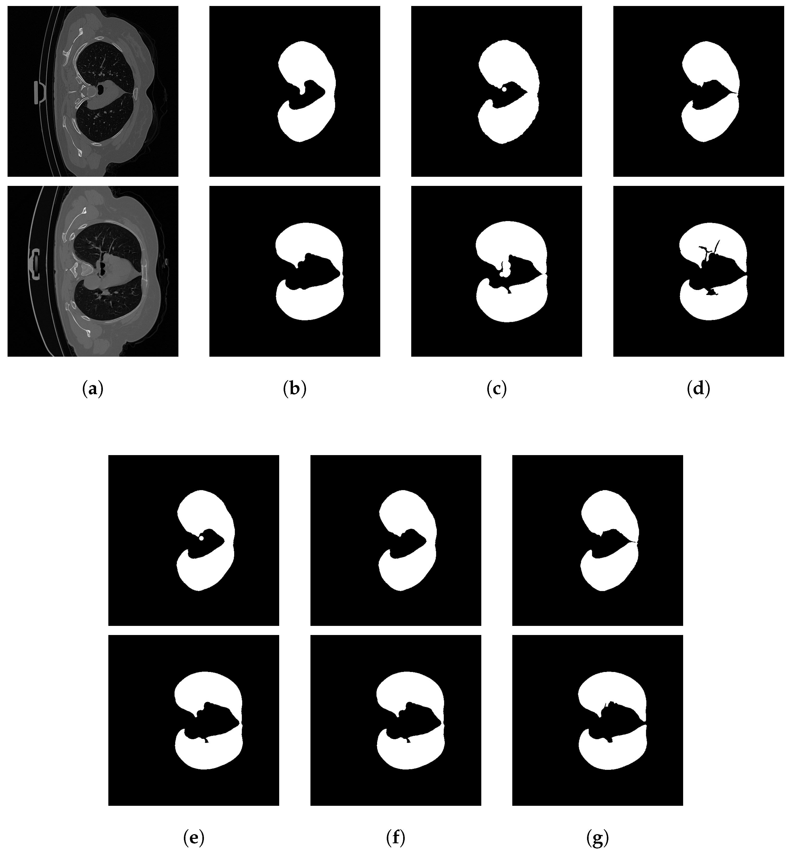
for the corresponding results. It can be observed that the post-processing step significantly improves the $\overline{F_1}$ and $\overline{MCC}$ values. It is also shown that despite the simplicity of the ensemble members, the segmentation performance is not far behind the performance of a DL method. For examples of the output of the ensemble and its members, see Figure 4.

4.7. Implementation and Hardware Details

All segmentation algorithms were implemented in Python and all optimization algorithms were implemented in Matlab. The outputs of the algorithms were computed offline and stored in memory during the optimization process along with the corresponding ground truth to reduce the time required to find a solution. The runtimes reported do not include the time required to load the ground truth and the outputs of the algorithms, nor any other overheads. Results for the dataset were obtained using a computer equipped with a 4-core 8-thread AMD Ryzen 3 3100 processor and 32 GB of DDR4 RAM.

5. Discussion and Conclusions

In this paper, we proposed SA-CNE, an SA-based stochastic method for the parameter optimization of medical image segmentation ensembles that combines dataset sampling and image downscaling to implement the noisy evaluation of the energy. By optimizing the parameters of a lung segmentation ensemble, we have shown that the proposed search method is capable of finding solutions with the same quality as the standard SA but with a significantly lower time requirement.

SA-CNE was shown to maintain the solution quality of the base method, yielding an $\overline{F_1}$ score of 0.7955 (0.9395 in lung segmentation with post-processing) and an associated $\overline{MCC}$ of 0.7736 (0.7755), compared to an $\overline{F_1}$ score of 0.7954 (0.9397) and an $\overline{MCC}$ of 0.7735 (0.7757) achieved by SA, while reducing the runtime by 42.01%.

We highlight that for a given problem, the combined evaluation method reverts to the sampling-based method above a certain dataset size $N_p$. Therefore, the proposed search method using the combined strategy is never less efficient than SA-SBE in terms of evaluation cost and is always more efficient than SA-SBE when the dataset size is smaller than $N_p$.

Considering real-world implementations, using the combined strategy instead of SA-SBE for datasets larger than $N_p$ implies negligible computational overhead during the search. However, in this case, generating and storing the pyramid representations of the dataset images is unnecessary. For this reason, it is beneficial to determine in advance which method is more appropriate for a given problem by calculating the total cost of search with the two methods for the size of the dataset.

One limitation of this study is that the proposed method was tested on a specific dataset and optimization task only. Therefore, further research is needed to explore its potential using different datasets and problems.

Despite the widespread adoption of DL methods, exploring the efficient optimization of traditional algorithms remains valuable. DL techniques have shown remarkable success in image segmentation tasks when abundant annotated data are available. However, obtaining annotated data can be expensive and time-consuming. Recently, there has been a growing interest in generating weak annotations with traditional algorithms. Using ensemble methods to combine such algorithms and optimizing their parameters at the system level can significantly improve the quality of their output without the need for further annotated data, which can ultimately benefit the training of DL models for image segmentation.

In conclusion, an efficient stochastic search method was proposed for optimizing medical image segmentation ensembles in this paper. SA-CNE demonstrated the ability to maintain the achievable solution by considering a given number of iterations while significantly reducing the computational time required for optimization compared to the standard SA. This work highlights the potential of using controlled noise in stochastic optimization methods.